Free and Forced Vibration Analysis of Two-Dimensional Linear Elastic Solids Using the Finite Element Methods Enriched by Interpolation Cover Functions

Abstract

In this paper, a novel enriched three-node triangular element with the augmented interpolation cover functions is proposed based on the original linear triangular element for two-dimensional solids. In this enriched triangular element, the augmented interpolation cover functions are employed to enrich the original standard linear shape functions over element patches. As a result, the original linear approximation space can be effectively enriched without adding extra nodes. To eliminate the linear dependence issue of the present method, an effective scheme is used to make the system matrices of the numerical model completely positive-definite. Through several typical numerical examples, the abilities of the present enriched three node triangular element in forced and free vibration analysis of two-dimensional solids are studied. The results show that, compared with the original linear triangular element, the present element can not only provide more accurate numerical results, but also have higher computational efficiency and convergence rate.

1. Introduction

Finite element method (FEM) [1,2,3] is a mature and powerful numerical method, which has become one of the most widely used numerical approaches in practical engineering applications because of its effectiveness and stability. However, the classical FEM also possesses several distinct disadvantages, for example, the computation accuracy of the classical FEM is relatively low when the low order linear elements are employed and the adaptability of FEM to mesh distortion is also relatively weak in the analysis of large deformation problems [4,5].

Note that the accuracy of the FEM solutions are seriously dependent on the quality of the used meshes, various the meshfree numerical techniques have also received lots of research interests in the past years [6,7,8,9,10,11,12,13,14,15]. The main difference between the standard FEM and the meshless numerical techniques is that the used shape functions are constructed using the scattered field nodes in the problem domain rather than relying on the pre-defined element. As a result, the approximation of the considered field variables is also independent on the mesh. Actually, many meshless methods have been developed to solve various engineering problems. In contrast with the classical boundary element method [16,17] and several boundary-based discretization techniques [18,19,20,21,22,23,24,25], most of the meshless numerical techniques are the domain-based numerical techniques and can be formulated using the weak form or strong form of the governing partial differential equations (PDE). Several well-developed weak form meshfree techniques consist of the reproducing kernel particle method (RKPM) [26], the diffuse element method [27], the element-free Galerkin method [7,28,29], Galerkin/least squares FEM [30], the radial point interpolation method (RPIM) [6,31] and so on. In addition, the strong form based meshfree techniques have also been developed, such as the generalized finite difference method (GFDM) [32,33,34], the finite point method (FPM) [35,36] and various collocation techniques [37,38,39,40]. All of these different meshless techniques have their own associated merits, demerits and conditions of applicability. Very nice and detailed reviews on the developments of the meshless techniques can be found in the monographs [6]. Nevertheless, it should be pointed out that the meshless methods still can not match the classical FEM in terms versatility and flexibility in engineering applications and many challenging problems still remain unsolved so far.

In order to enhance the performance of the standard FEM in engineering computation, Liu et al. proposed the smoothed FEM (S-FEM) [41,42,43,44,45,46] which combines traditional FEM with the generalized strain smoothing techniques with a mathematic base on the novel G space theory. By invoking the novel G space theory and strain smoothing operations, the “overly-stiff” stiffness matrices of the standard FEM can be properly softened and then a softened numerical model with appropriate system stiffness can be obtained. A substantial numerical examples have demonstrated that the S-FEM possesses many excellent and attractive properties compared to traditional FEM, such as higher computation accuracy and efficiency, faster convergence rates and better adaptability to mesh distortion. According to the different ways in performing the strain smoothing operations, a series of different S-FEMs have been proposed including the cell-based smoothed FEM (CS-FEM) [47,48,49], edge-based smoothed FEM (ES-FEM) [50,51] and the node-based smoothed FEM (NS-FEM) [52,53]. All of these different S-FEMs possesses their own associated strengths and specific properties, and these different S-FEMs can be used in various engineering applications.

Different from the smoothed FEM, the present work offers another approach to enhance the behaviors of the linear element of standard FEM in solving the two-dimensional dynamic problems. In this work, the extra interpolation cover functions, which are constructed by suitable polynomial bases, are employed to enhance the original linear nodal shape functions. As a result, the original linear approximation space of the classical FEM can be markedly enriched and the gradient field of the considered problem can be described more accurately. The present numerical method, which is named as enriched finite element method (EFEM), has been introduced by Bathe and his co-workers in solving the wave propagation problems and static analysis of linear elastic solid mechanics [54,55,56,57]. The numerical experiments have shown that much more accurate numerical results can be produced with the present EFEM and the extra nodes are not required. In addition, it should be pointed out that it is quite flexible in constructing the enrichment cover functions according to the special problem considered. By using the polynomial bases and the harmonic trigonometric functions as the enrichment cover functions, Chai et al. have employed the EFEM to solve the transient wave propagations and acoustic problems [58,59,60]. The related numerical results shown that the numerical dispersion error can be markedly suppressed by the EFEM in wave analysis and much more stable and accurate numerical solutions can be obtained. Furthermore, the present approach has also been extended to shell analysis and adaptive analysis [61,62].

In this work, we mainly focus on using the EFEM with simple linear interpolation cover functions, which has relatively high computation efficiency and is also easy for numerical integration, to analyze the free and forced vibration problem of the two-dimensional solids. The abilities of the EFEM for two-dimensional dynamics analysis are carefully examined through several typical numerical experiments.

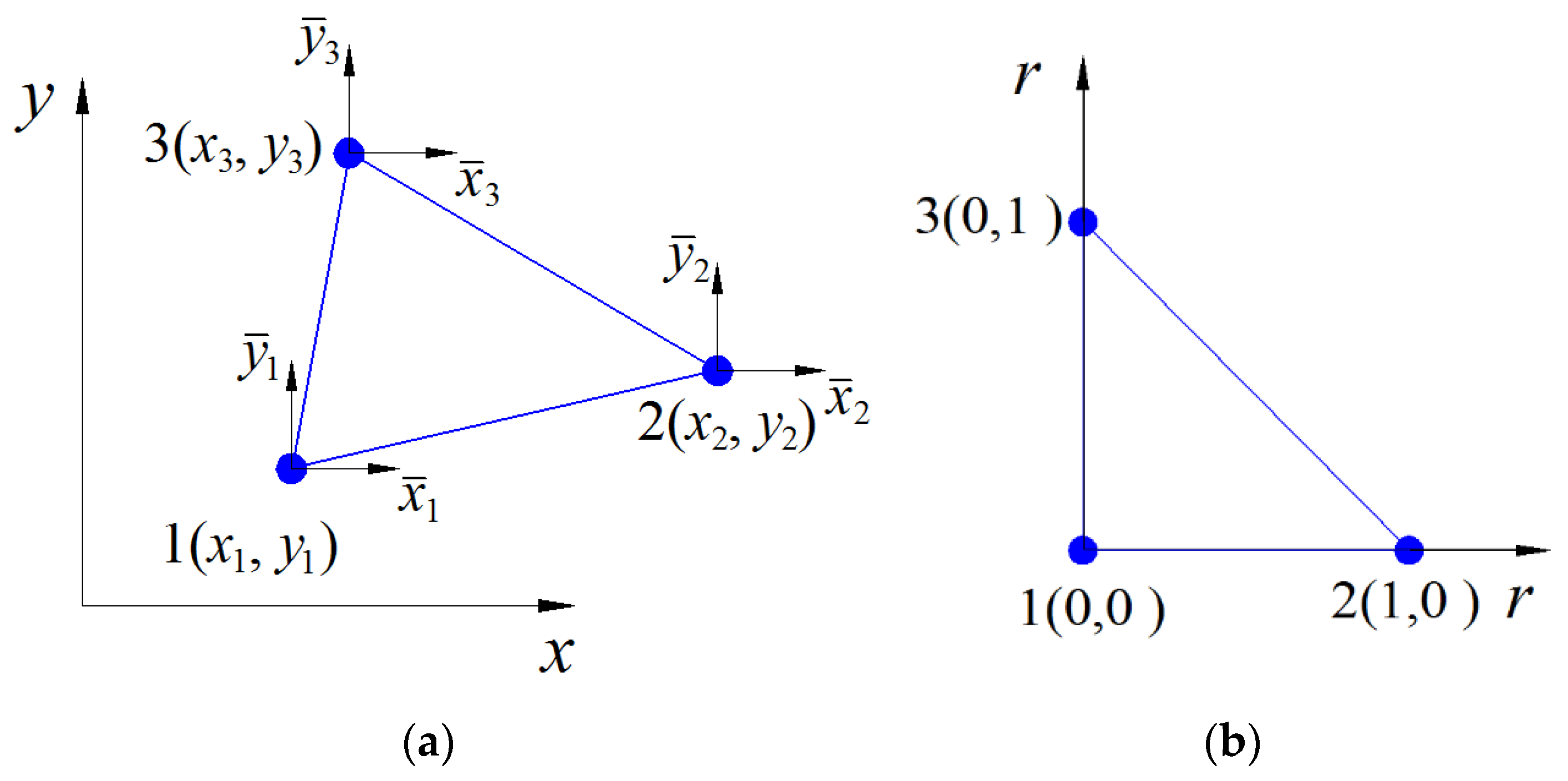
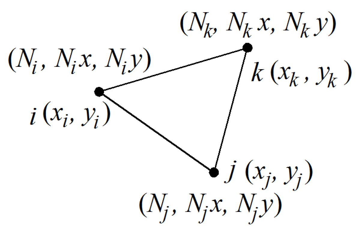
2. Formulation of the FEM Enriched by Interpolation Cover Functions

Consider a two-dimensional bounded problem domain. The standard N triangular elements are used to discretize the involved problem domain. Using the standard FE approximation, the interpolation for a scalar field function u has the following form

$$u={\displaystyle \sum _{i=1}^N{N}_i}{u}_i=\mathbf{N}\mathbf{u}$$

(1)

where u_i denotes the node coefficients of the field variable and N_i denotes the simple linear interpolation function for node i (see Figure 1a).

In the present enriched FE approximation, the standard triangular mesh is still used. As shown in Figure 1b, the union of all the elements attached to node i is defined as the cover region $C_i$ [56,58], it is actually the support domain of the usual linear nodal interpolation function for node i in the standard FE interpolation. Therefore, the element ε^m is also can be regarded as the overlapping region of the three surrounding cover region $C_i$, $C_j$ and $C_k$ (see Figure 1c). For the considered field variable u at node i, and the standard FE interpolation is enriched by the following expression [56,58],

$$E_i^q\left[u\right]=L{\left[\begin{array}{ccccc}{u}_i& a_{i1}& a_{i2}& a_{i3}& \cdots \end{array}\right]}^T$$

(2)

in which u_i is the usual nodal unknowns and ${\left[\begin{array}{cccc}{a}_{i1}& a_{i2}& a_{i3}& \cdots \end{array}\right]}^T$ denotes the additional unknowns which are associated with interpolation cover functions, L contains the polynomial bases of degree q.

$$L=\underset{\frac{\left(q+1\right)\left(q+2\right)}{2}\mathrm{terms}}{\underbrace{\left[\begin{array}{cccccccccccc}1& {\overline{x}}_i& {\overline{y}}_i& {\overline{x}}_i^2& {\overline{x}}_i{\overline{y}}_i& {\overline{y}}_i^2& {\overline{x}}_i^3& {\overline{x}}^2{}_i{\overline{y}}_i& {\overline{x}}_i{\overline{y}}_i^2& {\overline{y}}_i^3& \dots & {\overline{y}}_i^q\end{array}\right]}}$$

(3)

in which the used relative coordinate values $\left({\overline{x}}_i,{\overline{y}}_i\right)$ are defined in Figure 2, namely ${\overline{x}}_i=x-x_i$ and ${\overline{y}}_i=y-y_i$.

For the convenience of the comparison with the standard FE formulation, Equation (2) can also be expressed as [56,58],

$$E_i^q\left[u\right]=u_i+\underset{\mathrm{additional}\mathrm{interpolation}\mathrm{covers}}{\underbrace{{\left[\begin{array}{ccccccc}{\overline{x}}_i& {\overline{y}}_i& {\overline{x}}_i^2& {\overline{x}}_i{\overline{y}}_i& {\overline{y}}_i^2& \dots & {\overline{y}}_i^q\end{array}\right]}_{1\times \left[\frac{\left(q+1\right)\left(q+2\right)}{2}-1\right]}{\left[\begin{array}{c}{a}_{i1}\\ a_{i2}\\ a_{i3}\\ ⋮\end{array}\right]}_{\left[\frac{\left(q+1\right)\left(q+2\right)}{2}-1\right]\times 1}}}$$

(4)

From Equation (4), it is seen that the present EFEM formulation can be regarded as the standard FE approximation plus the additional enriched approximation.

Then the global approximation for the considered scalar field function $u$ has the following form [56,58],

$$T{E}_i^q\left[u\right]={\displaystyle \sum _1^m\left({\displaystyle \sum _{i=1}^3{N}_i{E}_i^q\left[u\right]}\right)}={\displaystyle \sum _1^m\left({\displaystyle \sum _{i=1}^3{N}_i{u}_i+{\displaystyle \sum _{i=1}^3{H}_i{a}_i}}\right)}={\displaystyle \sum _1^m\left({\displaystyle \sum _{i=1}^3{N}_i{u}_i+{\displaystyle \sum _{i=1}^3{\displaystyle \sum _{j=1}^n{H}_{i,j}{a}_{i,j}}}}\right)},$$

(5)

where m stands for the number of all nodes in the problem domain, N_i denotes the original linear interpolation functions, j represents the added degree of freedoms (DOFs) for each node, $H$ is the obtained hybrid interpolation function matrix.

$$H_i=N_i\left[\begin{array}{ccccccccccc}{\overline{x}}_i& {\overline{y}}_i& {\overline{x}}_i^2& {\overline{x}}_i{\overline{y}}_i& {\overline{y}}_i^2& {\overline{x}}_i^3& {\overline{x}}^2{}_i{\overline{y}}_i& {\overline{x}}_i{\overline{y}}_i^2& {\overline{y}}_i^3& \dots & {\overline{y}}_i^q\end{array}\right]$$

(6)

From above formulation, it can be found that the present EFEM will become the standard FEM if the employed polynomial bases only contains the constant term 1. With this operation, the higher order approximation space can be constructed and then leads to much higher computation accuracy. Since the original linear nodal shape functions and the constructed hybrid nodal shape functions have the totally identical supports, the proposed EFEM is also able to lead to the sparse system matrices as in the standard FEM.

Actually we can employ any order of polynomial bases as the interpolation cover functions. More accurate numerical results can also be generated if the high order polynomial interpolation cover functions are employed. However, the high order interpolation cover functions will result in more nodal unknowns and more computational cost. In this work, we only use the first order polynomial bases [1 x y] (q = 1) as the interpolation cover functions. Note that three additional DOFs will be introduced for each node when the first order polynomial bases are used, hence in this work the abbreviation EFEM-N3 is used to represent the EFEM with linear interpolation cover functions.

For the plane stress problem considered in this work, the displacement field variables u and v in element ε^m (see Figure 1) can be obtained as following based on the above EFEM-N3 formulation [56],

$$u_h^m={\displaystyle \sum _{i=1}^3\left(N_i{u}_i+H_i{a}_i^u\right)},v_h^m={\displaystyle \sum _{i=1}^3\left(N_i{v}_i+H_i{a}_i^v\right)},$$

(7)

$${\left(a_i^u\right)}^T=\left[\begin{array}{cc}{a}_{i1}^u& a_{i2}^u\end{array}\right],{\left(a_i^v\right)}^T=\left[\begin{array}{cc}{a}_{i1}^v& a_{i2}^v\end{array}\right],$$

(8)

in which $u_i$ and $v_i$ are the usual nodal unknowns as in the standard FEM, $a_i^u$ and $a_i^v$ are the vectors which contain additional unknowns.

Actually Equation (7) can also be expressed in the following matrix form when the first order polynomial bases [1 x y] are used as the interpolation cover functions,

$$\left[\begin{array}{c}{u}_h^m\\ v_h^m\end{array}\right]=\left[\begin{array}{cc}\begin{array}{cc}\mathbf{N}& \mathbf{H}\\ {\mathbf{0}}_{1\times 3}& {\mathbf{0}}_{1\times 6}\end{array}& \begin{array}{cc}{\mathbf{0}}_{1\times 3}& {\mathbf{0}}_{1\times 6}\\ \mathbf{N}& \mathbf{H}\end{array}\end{array}\right]\left[\begin{array}{l}\begin{array}{c}\mathbf{u}\\ {\mathbf{a}}_u\end{array}\\ \begin{array}{c}\mathbf{v}\\ {\mathbf{a}}_v\end{array}\end{array}\right]$$

(9)

in which $\mathbf{N}$ is the usual linear interpolation function matrix for the standard FEM $H$ is the constructed hybrid interpolation function matrix for the present EFEM-N3. To improve the conditioning of the present EFEM-N3 and obtain more stable numerical solutions, the additional unknowns coefficients are normalized by a/h in this work (in which h denotes the average mesh size of the used mesh pattern).

Similar as in the standard FE scheme, the related derivatives of the displacement variable can be obtained using the following usual differentiation rules,

$$\left[\begin{array}{l}{u}_{h,x}^m\\ u_{h,y}^m\end{array}\right]=\left[\begin{array}{cc}{N}_{,x}& H_{,x}\\ N_{,y}& H_{,y}\end{array}\right]\left[\begin{array}{l}u\\ a_u\end{array}\right],\left[\begin{array}{l}{v}_{h,x}^m\\ v_{h,y}^m\end{array}\right]=\left[\begin{array}{cc}{N}_{,x}& H_{,x}\\ N_{,y}& H_{,y}\end{array}\right]\left[\begin{array}{l}v\\ a_v\end{array}\right],$$

(10)

in which,

$$\left[\begin{array}{cc}{N}_{,x}& H_{,x}\\ N_{,y}& H_{,y}\end{array}\right]=J^{-1}\left[\begin{array}{cc}{N}_{,r}& H_{,r}\\ N_{,s}& H_{,s}\end{array}\right]$$

(11)

in which $J$ is the Jacobian matrix and the required coordinate transformation can be achieved as similarly as in the standard FE scheme (see Figure 2b).

3. Governing Equations of Dynamics for Linear Elastic Solids

For the two-dimensional linear elastic solid mechanic problems defined in a bounded domain $\mathsf{\Omega }$. The standard Galerkin weak form is as follows [2],

$${\displaystyle {\int }_{\mathsf{\Omega }}{\left(\nabla \delta u\right)}^T}D\left(\nabla u\right)\mathrm{d}\mathsf{\Omega }-{\displaystyle {\int }_{\mathsf{\Omega }}\delta u^T\left(b-\rho \ddot{u}-c\dot{u}\right)}\mathrm{d}\mathsf{\Omega }-{\displaystyle {\int }_{{\mathsf{\Gamma }}_N}\delta u^{T}t}\mathrm{d}\mathsf{\Gamma }=0$$

(12)

in which $\nabla$ is the differential operator, $\delta u$ is the arbitrary virtual displacement vector, $D$ is the material constant matrix, $b$ denotes the body force vector, $\ddot{u}$ and $\dot{u}$ are the acceleration and velocity vectors, $\rho$ and c are the density and damping coefficients of the considered solids, ${\mathsf{\Gamma }}_N$ is the natural boundary condition and t is the prescribed traction vector on ${\mathsf{\Gamma }}_N$.

Using the EFEM interpolation shown in Equation (7), the matrix form of Equation (12) can be obtained by,

$$M\ddot{u}+C\dot{u}+Ku=f$$

(13)

$$M={\displaystyle \sum _{i=1}^{n_e}{\displaystyle {\int }_{{\mathsf{\Omega }}_i}{N}_i^T}\rho N_i\mathrm{d}\mathsf{\Omega }},C={\displaystyle \sum _{i=1}^{n_e}{\displaystyle {\int }_{{\mathsf{\Omega }}_i}{N}_i^T}c{N}_i\mathrm{d}\mathsf{\Omega }},K={\displaystyle \sum _{i=1}^{n_e}{\displaystyle {\int }_{{\mathsf{\Omega }}_i}{B}_i^T}D{B}_i\mathrm{d}\mathsf{\Omega }}$$

(14)

$$f={\displaystyle \sum _{i=1}^{n_e}{\displaystyle {\int }_{{\mathsf{\Omega }}_i}{N}_i^{T}b}\mathrm{d}\mathsf{\Omega }+{\displaystyle \sum _{i=1}^{n_b}{\displaystyle {\int }_{{\mathsf{\Gamma }}_N}{N}_i^{T}t}\mathrm{d}\mathsf{\Gamma }}},D=\frac{E}{1-v^2}\left[\begin{array}{ccc}1& v& 0\\ v& 1& 0\\ 0& 0& \frac{1-v}{2}\end{array}\right]$$

(15)

in which $M$ is the global mass matrix, n_e is the total number of elements in the global mesh and ${\mathsf{\Omega }}_i$ denotes element i, n_b is the number of elements on the Neumann boundary, $N_i$ is the involved shape function matrix for element i, $C$ is the matrix containing the damping effects, $K$ is the global stiffness matrix, E is Young’s modulus and v is Poisson’s ratio, $D$ is a matrix containing the material parameters, B_i is the strain gradient matrix for element i, $f$ is the related nodal force vector.

From the formulation in Section 2, the shape function matrix $N_t$ and strain gradient matrix B for two-dimensional solid mechanics can be obtained by,

$$N_t=\left[\begin{array}{cccc}N& H& 0_{1\times 3}& 0_{1\times 6}\\ 0_{1\times 3}& 0_{1\times 6}& N& H\end{array}\right],$$

(16)

$$B=\nabla N_t=\left[\begin{array}{cccc}\partial N/\partial x& \partial H/\partial x& 0_{1\times 3}& 0_{1\times 6}\\ 0_{1\times 3}& 0_{1\times 6}& \partial N/\partial y& \partial H/\partial y\\ \partial N/\partial y& \partial H/\partial y& \partial N/\partial x& \partial H/\partial x\end{array}\right],$$

(17)

For the convenience of discussion, the Rayleigh damping is employed here and the damping matrix C is obtained directly from the mass matrix M and stiffness matrix K by,

$$C=\alpha M+\beta K$$

(18)

in which $\alpha$ and $\beta$ stand for the Rayleigh damping coefficients.

If the damping effects are not considered, for free vibration analysis Equation (13) can be re-written by,

$$M\ddot{u}+Ku=0$$

(19)

It is easy to find that Equation (19) has the following fundamental solution,

$$u=\overline{u}\exp \left(j\omega t\right)$$

(20)

in which $\overline{u}$ is the amplitude of displacement distributions in two dimensions, $j=\sqrt{-1}$ and $\omega$ is the angular frequency.

Taking Equation (20) into Equation (19), we can arrive at,

$$\left[K-{\omega }^{2}M\right]\overline{u}=0$$

(21)

It is indicated in Equation (21) that the essence of analyzing the free vibration problems is to solve the typical eigenvalue problem.

For forced vibration analysis, we actually should solve the second-order time-dependent dynamic problems which is governed by the matrix equation shown Equation (13). In practice, many different types of direct time integration schemes have been developed for solving the structural dynamic problems, here the widely used Newmark method, which is an unconditionally stable direct time integration technique, is used for the analysis of dynamic problems, the following assumptions are used in the Newmark method,

$$\{\begin{array}{l}{}^{t+\mathsf{\Delta }t}\dot{u}={}^t\dot{u}+\left[\left(1-\delta \right){}^t\ddot{u}+\delta {}^{t+\mathsf{\Delta }t}\ddot{u}\right]\mathsf{\Delta }t\\ {}^{t+\mathsf{\Delta }t}u={}^{t}u+{}^t\dot{u}\mathsf{\Delta }t+\left[\left(\frac{1}{2}-\alpha \right){}^t\ddot{u}+\alpha {}^{t+\mathsf{\Delta }t}\ddot{u}\right]\mathsf{\Delta }{t}^2\end{array}$$

(22)

in which $\mathsf{\Delta }t$ stands for the time step for time integration, $\delta$ and $\alpha$ are the undetermined coefficients which are related to the integration accuracy.

In addition, the following equilibrium equation at time $t+\mathsf{\Delta }t$ should also be used,

$$M{}^{t+\mathsf{\Delta }t}\ddot{u}+C{}^{t+\mathsf{\Delta }t}\dot{u}+K{}^{t+\mathsf{\Delta }t}u={}^{t+\mathsf{\Delta }t}f$$

(23)

Since no numerical damping effects will be introduced to the numerical solution when $\delta =\frac{1}{2}$ and $\alpha =\frac{1}{4}$, so these two parameters are used in this work. Combining Equations (22) and (13), at time $t+\mathsf{\Delta }t$ we can obtain [2],

$$\left(\frac{4}{\mathsf{\Delta }{t}^2}M+\frac{2}{\mathsf{\Delta }t}C+K\right){}^{t+\mathsf{\Delta }t}u={}^{t+\mathsf{\Delta }t}f+M\left(\frac{4}{\mathsf{\Delta }{t}^2}{}^{t}u+\frac{4}{\mathsf{\Delta }t}{}^t\dot{u}+{}^t\ddot{u}\right)+C\left(\frac{2}{\mathsf{\Delta }t}{}^{t}u+{}^t\dot{u}\right),$$

(24)

Then the complete numerical solution can be finally obtained by recursively using Equations (22)–(24).

4. The Linear Dependence Issue

We have known that one major issue in the EFEM formulation is the linear dependence (LD) issue of the obtained system discretized equations [56,58]. To obtain stable numerical solution, this linear dependence issue should be addressed carefully. Actually, the origin of the involved linear dependence issue in EFEM is that the approximation of the considered field variable is constructed by employing the linear dependent shape functions, hence the obtained system matrices are usually singular. To address the LD problem of the EFEM and make the obtained system matrices to be positive definite, Kim and Bathe directly remove all the cover DOFs on the Dirichlet boundary and it is shown that the linear dependence issue indeed can be completely removed [56]. However, the overly-constrained global discretized equations are actually obtained with this operation and in essence we do not need to remove all the cover DOFs on the Dirichlet boundary. In consequence, this operation always lead to the unnecessary loss of computation accuracy. In this work, we use a new scheme to address the LD of the EFEM. In this scheme, the minimum superfluous cover DOFs are eliminated to ensure that the resultant global system matrices are completely positive definite, hence the computation accuracy can be largely maintained. Furthermore, due to the linear dependence issue the imposition of the Dirichlet boundary condition in the EFEM is quite different from that in the standard FEM, hence the accurate imposition of the Dirichlet boundary condition in the EFEM framework is also discussed in detail within this work.

If the first order complete polynomials are employed as the cover functions, in the EFEM formulation we can obtain nine nodal shape functions for each triangular element. (see Figure 3).

Here $N_l$ (l = i, j, k) represent the conventional linear interpolation functions in a standard linear triangular element.

$$\{\begin{array}{l}{N}_i=\frac{1}{2A}\left[\left(x_j{y}_k-x_k{y}_j\right)+\left(y_j-y_k\right)x+\left(x_k-x_j\right)y\right]\\ N_j=\frac{1}{2A}\left[\left(x_k{y}_i-x_i{y}_k\right)+\left(y_k-y_i\right)x+\left(x_i-x_k\right)y\right]\\ N_k=\frac{1}{2A}\left[\left(x_i{y}_j-x_j{y}_i\right)+\left(y_i-y_j\right)x+\left(x_j-x_i\right)y\right]\end{array}$$

(25)

From Ref. [58], we can obtain the following theorem.

Theorem 1.

For the approximation space spanned by the nine shape functions in Figure 3,$\mathrm{span}\left\{\begin{array}{ccccccccc}{N}_i& N_j& N_k& N_{i}x& N_{j}x& N_{k}x& N_{i}y& N_{j}y& N_{k}y\end{array}\right\}=\mathrm{span}\left\{\begin{array}{cccccc}1& x& y& x^2& xy& y^2\end{array}\right\}$.

The related proofs for the above theorem are not given here, more details can be found in Ref. [58]. Based on Theorem 1 and the related analysis in Ref. [58], it is known that the five nodal shape functions $\mathrm{span}\left\{\begin{array}{ccccc}{N}_i& N_j& N_k& N_{i}x& N_{j}x\end{array}\right\}$ are definitely linear independent and $\mathrm{span}\left\{\begin{array}{ccccc}{N}_i& N_j& N_k& N_{i}x& N_{j}x\end{array}\right\}=\mathrm{span}\left\{\begin{array}{ccccc}1& x& y& x^2& xy\end{array}\right\}$, hence another term in $\left\{\begin{array}{ccc}{N}_{i}y& N_{j}y& N_{k}y\end{array}\right\}$ in which the $y^2$ term is contained should be found out, then the completely quadratic approximation space can be obtained. From Equation (25), it is clear that any one in $\left\{\begin{array}{ccc}{N}_{i}y& N_{j}y& N_{k}y\end{array}\right\}$ will contain the $y^2$ term and can be used when $x_i\ne x_j\ne x_k$. However, $N_{i}y$ or $N_{k}y$ can be used when $x_i=x_k$, $N_{i}y$ or $N_{j}y$ can be used when $x_i=x_j$.

From Ref. [58], we also can obtain the following theorem.

Theorem 2.

For the normal mesh without singular node, once the six linearly independent shape functions are used for any single element, the LD of the obtained system discretized equations based on the global mesh will be completely removed.

Using Theorems 1 and 2, the linear dependence problem of the EFEM can be can be completely removed without any loss in computation accuracy.

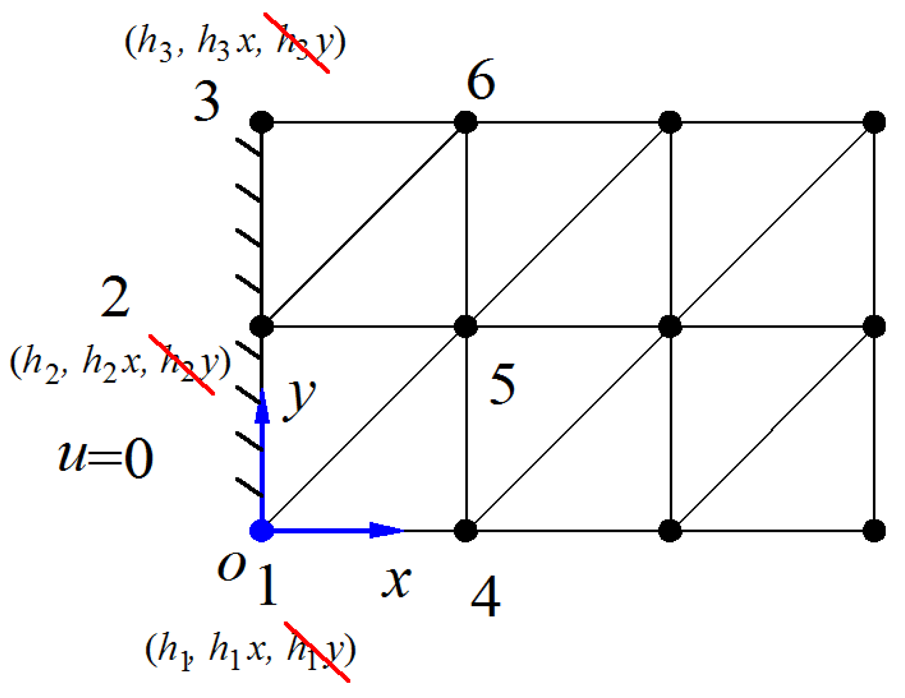
5. Imposition of the Dirichlet Boundary Condition

We have known that the natural boundary condition (BC) can be directly imposed in the EFEM which is quite similar as in the conventional FEM [56,58]. However, the Dirichlet BC cannot be imposed directly in the EFEM and should be carefully discussed.

Taking the mesh pattern in Figure 4 for example, the Dirichlet BC u = 0 for a considered scalar field is prescribed on x = 0. To accurately apply this Dirichlet BC, all the y cover DOFs should be firstly eliminated. Furthermore, to address the linear dependence issue, in the global mesh six linear independent shape functions which can exactly construct the complete quadratic approximation space should be employed for at least one triangular element. This kind of element should be determined very carefully based on Theorem 1.

For instance, when we choose the element 1-5-2 as the initial element. Due to the Dirichlet BC u = 0 on x = 0, two y cover DOFs $N_{1}y$ and $N_{2}y$ should be firstly eliminated, then the remaining nodal shape functions for element 1-5-2 are $\left\{\begin{array}{ccccccc}{N}_1& N_5& N_2& N_{1}x& N_{5}x& N_{2}x& N_{5}y\end{array}\right\}$. Note that $x_1=x_2$ here, so the shape function $N_{5}y$ will not contain $y^2$ term, hence $\mathrm{span}\left\{\begin{array}{ccccccc}{N}_1& N_5& N_2& N_{1}x& N_{5}x& N_{2}x& N_{5}y\end{array}\right\}$$\ne \mathrm{span}\left\{\begin{array}{cccccc}1& x& y& x^2& xy& y^2\end{array}\right\}$, namely the element 1-5-2 is not appropriate as the initial element which should have six linearly independent shape functions to eliminate the linear dependence issue.

However, the element 1-4-5 is appropriate as the initial element. Due to the Dirichlet BC u = 0 on x = 0, the y cover DOF $N_{1}y$ should be firstly eliminated. Based on the analysis in Section 3, it is clear that the following six nodal shape functions $\left\{\begin{array}{cccccc}{h}_1& h_4& h_5& h_{1}x& h_{4}x& h_{5}y\end{array}\right\}$ are linearly independent and $\left\{\begin{array}{cccccc}{h}_1& h_4& h_5& h_{1}x& h_{4}x& h_{5}y\end{array}\right\}$=$\mathrm{span}\left\{\begin{array}{cccccc}1& x& y& x^2& xy& y^2\end{array}\right\}$.

Finally, the linear dependence problem of the EFEM can be completely removed using above analysis and discussion, and the Dirichlet BC can also be accurately imposed.

6. Numerical Results

Several supporting numerical experiments will be considered in this section to assess the abilities of the proposed method for free and forced vibration analysis of two-dimensional linear elastic solids.

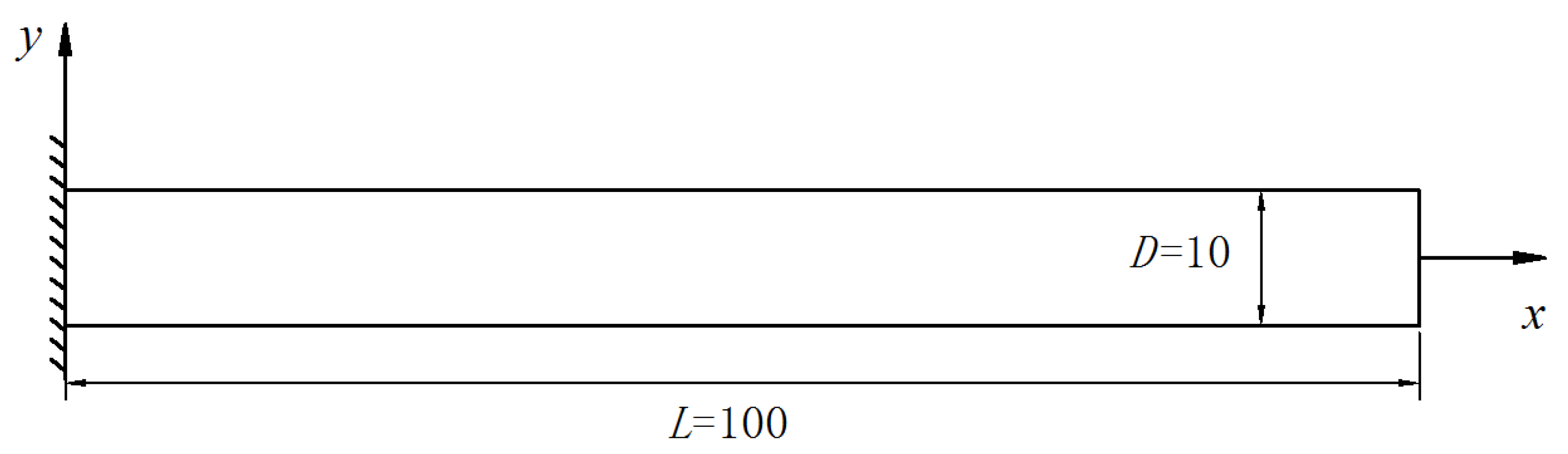
6.1. Free Vibration Analysis of a Cantilever Beam

The first considered numerical example is a cantilever beam. As shown in Figure 5, the geometry parameters of this cantilever beam is thickness t = 1, width D = 10 and length L = 100. The plane stress condition is considered here and the related material parameters are Poisson’s ratio v = 0.3, Young’s modulus E = 2.1 × 10¹¹ and mass density $\rho$ = 8 × 10⁻¹⁰. This is a very common benchmark problem in the free vibration analysis and has been investigated detailedly by many researchers using different numerical methods [63,64].

6.1.1. Computation Accuracy Study

To examine the behaviors of the present EFEM-N3 in free vibration analysis, a series of standard regular triangular mesh with different average element sizes (see Figure 6) are employed in the numerical computation. The first 10 natural frequencies calculated by the linear triangular element (FEM-T3), bilinear quadrilateral element (FEM-Q4), the edge-based smoothed FEM (ES-FEM) [41,50] and the present EFEM-N3 are given in

Table 1. The natural frequency solutions from different elements using Mesh 1 (22 nodes, 20 elements).

Mode	FEM-T3	FEM-Q4	ES-FEM	EFEM-N3	Reference
1	1704.07	999.94	1060.41	826.44	822.41
2	9550.05	6077.08	6486.92	4997.09	4932.71
3	12,898.51	12,863.12	12,879.18	12,833.79	12,823.96
4	23,636.40	16,422.55	17,676.71	13,310.92	12,993.08
5	38,878.90	30,961.53	33,611.81	24,522.67	23,611.65
6	40,960.87	38,921.06	39,070.31	37,946.19	36,009.93
7	60,074.90	49,338.69	54,156.41	38,482.34	38,443.95
8	66,226.33	65,982.06	66,621.04	53,047.17	49,578.22
9	81,228.50	71,244.04	79,745.90	64,058.56	63,912.57
10	94,589.79	94,728.11	96,638.13	69,457.19	63,974.64

,

Table 2. The natural frequency solutions from different elements using Mesh 2 (63 nodes, 80 elements).

Mode	FEM-T3	FEM-Q4	ES-FEM	EFEM-N3	Reference
1	1119.29	871.76	855.74	823.84	822.41
2	6617.08	5263.48	5180.43	4944.89	4932.71
3	12,849.69	12,837.12	12,840.31	12,827.62	12,823.96
4	17,162.01	14,010.46	13,829.41	13,038.27	12,993.08
5	30,745.07	25,816.34	25,565.29	23,729.46	23,611.65
6	38,620.23	38,573.48	38,608.10	36,259.33	36,009.93
7	46,401.47	40,002.13	39,764.95	38,455.45	38,443.95
8	63,385.94	56,042.63	55,964.71	50,037.34	49,578.22
9	64,681.80	64,493.66	64,650.99	63,995.63	63,912.57
10	81,520.49	73,610.95	73,943.12	64,678.33	63,974.64

and

Table 3. The natural frequency solutions from different elements using Mesh 3 (205 nodes, 320 elements).

Mode	FEM-T3	FEM-Q4	ES-FEM	EFEM-N3	Reference
1	906.83	835.16	827.37	822.74	822.41
2	5425.61	5019.96	4975.61	4935.85	4932.71
3	12,833.24	12,828.32	12,828.93	12,825.28	12,823.96
4	14,254.61	13,263.55	13,150.15	13,002.27	12,993.08
5	25,852.78	24,200.63	23,997.99	23,631.32	23,611.65
6	38,493.15	37,078.50	36,775.32	36,045.90	36,009.93
7	39,398.63	38,479.58	38,488.49	38,447.96	38,443.95
8	54,244.91	51,308.85	50,906.49	49,637.97	49,578.22
9	64,160.33	64,109.88	64,146.76	63,980.08	63,912.57
10	70,011.80	66,507.56	66,022.83	64,006.94	63,974.64

. For comparison, the numerical results using the commercial software package ABAQUS with a very fine triangular mesh (4221 nodes and 8000 elements) are also listed in the tables as the reference solutions. We can see that the numerical errors of the natural frequencies from the standard FEM-T3 and FEM-Q4 are relatively large. This is because the computation accuracy of the low order linear elements in the standard FEM is not sufficiently high, especially when the relatively coarse meshes are used. The ES-FEM solutions are clearly better than those from the standard FEM, while the proposed EFEM-N3 can provide the most accurate numerical results. In addition, it is also evident that the quality of numerical solutions from all four different numerical methods will become worse with the increase of the mode order. Nevertheless, the behaviors of the present EFEM-N3 are markedly better than other methods. Furthermore, the first 10 mode shapes of the cantilever beam from the EFEM-N3 are depicted in Figure 7, we can see that the physical vibration mode can be accurately predicted by the present EFEM-N3.

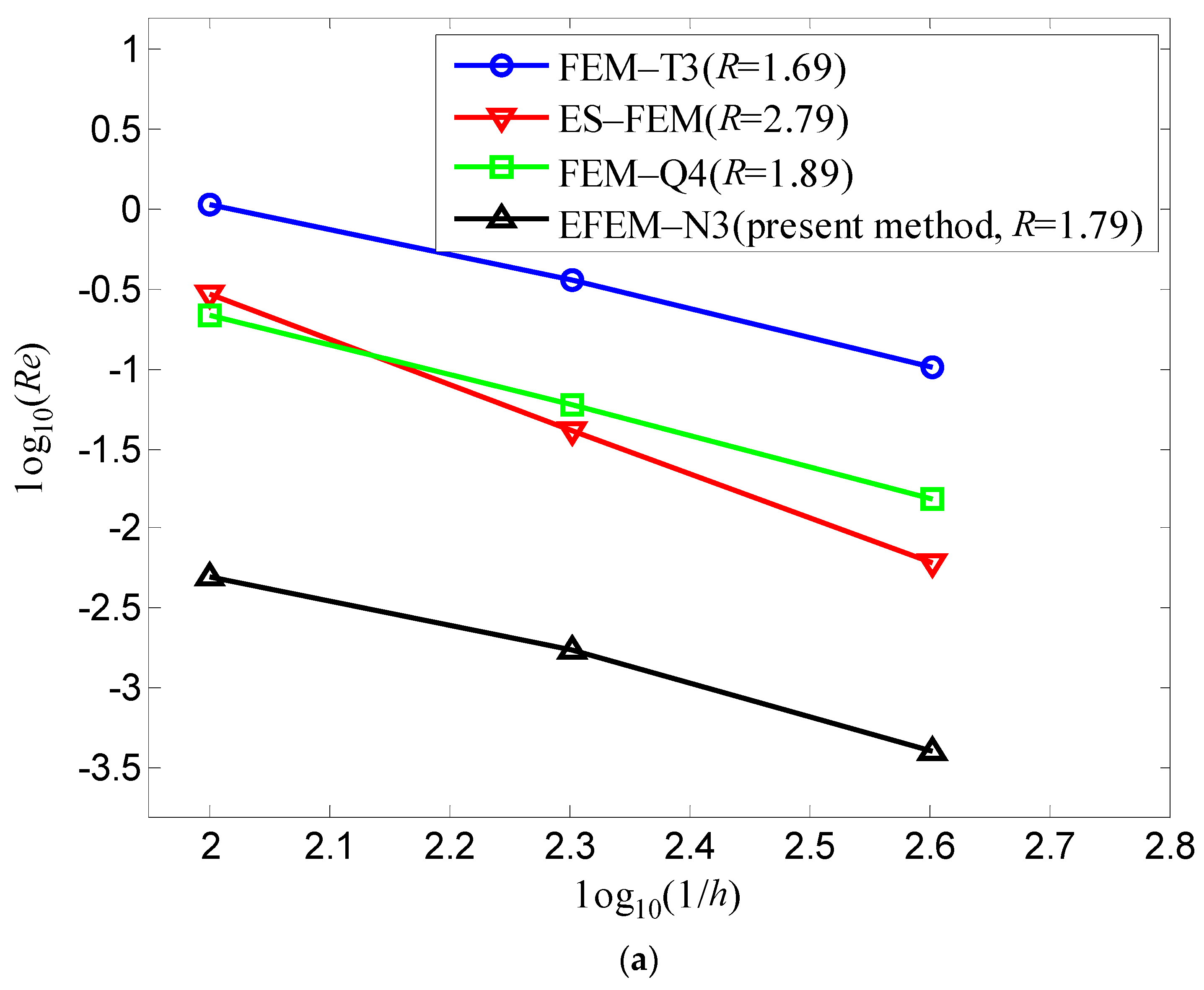
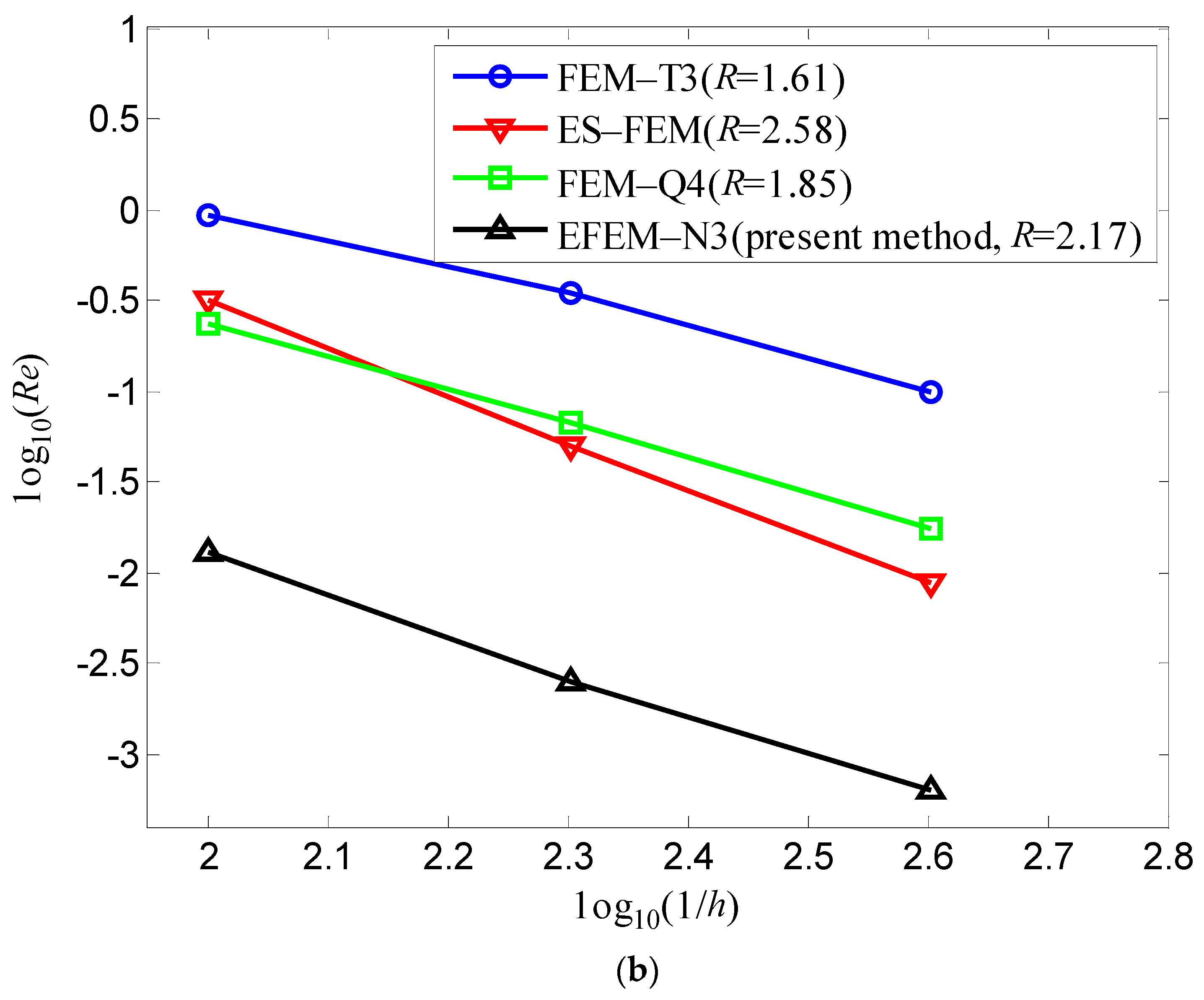
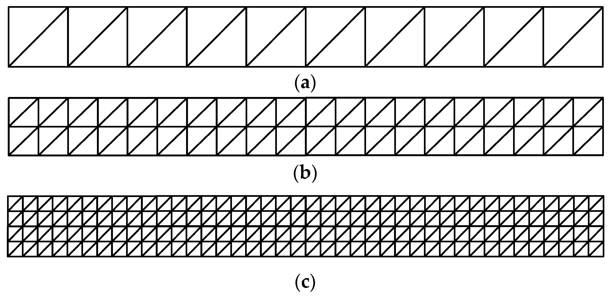
6.1.2. Convergence Study

Several uniform meshes with varying node intervals shown in Figure 6 are employed to assess the convergence properties of the different numerical approaches in free vibration analysis. The following relative error indicator for the calculated natural frequency results are used,

$$Re=\left|\frac{f^{{}_{num}}-f^{{}_{ref}}}{f^{{}_{ref}}}\right|\times 100\%$$

(26)

in which $f^{{}_{num}}$ and $f^{{}_{ref}}$ represent the natural frequency results from the different elements and the corresponding reference solutions, respectively.

For the first and second order vibration mode of the cantilever beam, the relative error indicator Re of the obtained natural frequency results from different elements versus the average meshsize h are plotted in Figure 8. It can be found that the ES-FEM shows better convergence properties than the proposed EFEM-N3. Nevertheless, the convergence rate of the present EFEM-N3 is still markedly higher than the standard FEM.

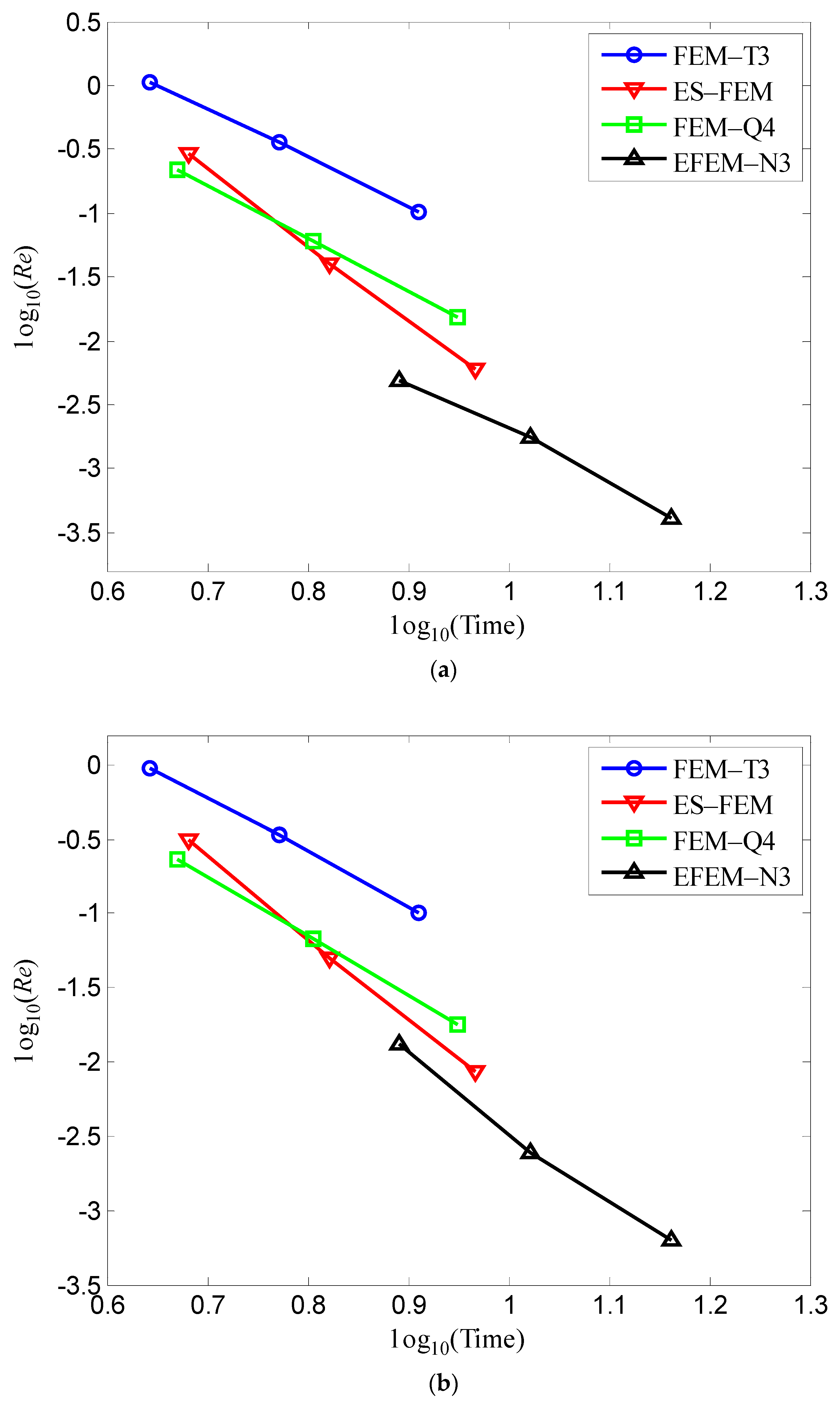
6.1.3. Computation Efficiency Study

Now we have known that the EFEM-N3 behaves better than the traditional FEM in computation accuracy and convergence rate for free vibration analysis. However, from the related formulation in Section 2 we can find that more nodal unknowns and more expensive numerical integration are involved in the present EFEM-N3 than the other elements. Here the uniform meshes shown in Figure 6 with different average meshsizes are again used and the first two natural frequency results are discussed to investigate the computation efficiency of the EFEM-N3. Figure 9 displays the corresponding relative error indicator results versus the solution time for different elements. We can see that the proposed EFEM-N3 is much more time-consuming compared to other methods when the same mesh pattern is used. However, the relative error indicator from the EFEM-N3 is the smallest for the same computational cost. These findings indicate that the EFEM-N3 has higher computation efficiency than the other three elements for free vibration analysis.

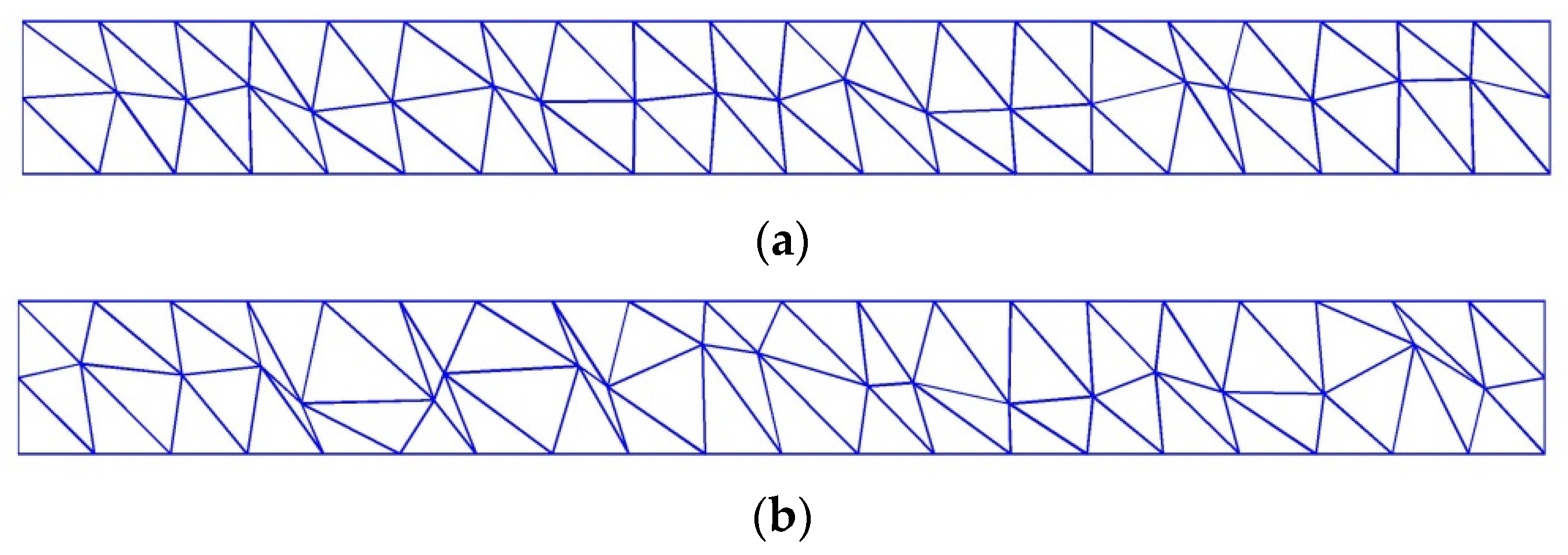
6.1.4. Effects of Mesh Distortion

In this section, we will evaluate the effects of the mesh distortion on the computation accuracy for different elements. Both uniform mesh with regular node distributions and distorted mesh with irregular node distributions are used here. The distorted mesh is directly obtained from the uniform mesh using the following treatments [47],

$$\{\begin{array}{l}{x}_{ir}=x_{re}+h\cdot r_c\cdot {\beta }_{ir}\\ y_{ir}=y_{re}+h\cdot r_c\cdot {\beta }_{ir}\end{array}$$

(27)

in which $x_{re}$ and $y_{re}$ are original node coordinate values of the uniform mesh, h is the average nodal space, $r_c\in \left[-1,1\right]$ is a random number, ${\beta }_{ir}\in \left[0,0.5\right]$ is a prescribed irregularity indicator, $x_{ir}$ and $y_{ir}$ are the node coordinate values of the obtained distorted mesh.

We can see from Figure 10 that the number of nodes is same for the uniform mesh and distorted mesh, and larger irregularity indicator ${\beta }_{ir}$ will lead to more distorted mesh.

Table 4. The calculated natural frequencies (Hz) from different elements using the distorted mesh shown in Figure 10a.

Mode	FEM-T3	FEM-Q4	ES-FEM	EFEM-N3	Reference
1	1122.20	880.70	863.63	823.81	822.41
2	6611.69	5314.24	5218.07	4945.35	4932.71
3	12,848.43	12,837.54	12,840.35	12,827.54	12,823.96
4	17,091.48	14,196.79	13,970.51	13,040.24	12,993.08
5	30,885.01	26,093.70	25,793.25	23,737.90	23,611.65
6	38,619.45	38,580.22	38,615.20	36,274.70	36,009.93
7	46,957.70	40,508.40	40,139.30	38,455.24	38,443.95
8	63,665.54	56,599.45	56,450.22	50,068.29	49,578.22
9	64,732.78	64,529.76	64,683.06	63,995.51	63,912.57
10	81,946.64	74,204.78	74,725.45	64,739.58	63,974.64

and

Table 5. The calculated natural frequencies (Hz) from different elements using the distorted mesh shown in Figure 10b.

Mode	FEM-T3	FEM-Q4	ES-FEM	EFEM-N3	Reference
1	1145.59	898.93	884.98	823.97	822.41
2	6737.77	5455.77	5369.86	4947.20	4932.71
3	12,853.75	12,837.90	12,843.17	12,828.10	12,823.96
4	17,179.78	14,586.04	14,420.32	13,050.46	12,993.08
5	31,362.44	26,581.86	26,471.00	23,766.85	23,611.65
6	38,629.17	38,580.54	38,633.98	36,352.11	36,009.93
7	47,501.75	40,940.73	40,865.35	38,457.08	38,443.95
8	63,711.47	57,399.92	57,474.63	50,197.60	49,578.22
9	64,801.35	64,531.84	64,743.80	63,998.94	63,912.57
10	82,916.05	75,850.72	76,237.81	64,908.02	63,974.64

list the first 10 natural frequency results from different elements using two distorted meshes (see Figure 10). For computation, the corresponding results from the uniform mesh and the reference solutions are also listed in the tables. From the results, it is seen that the computation accuracy of the standard linear elements (FEM-T3 and FEM-Q4) will degrade clearly when the distorted mesh pattern is employed. The performance of the ES-FEM is better than the traditional FEM, while the present EFEM-N3 behaves best among all the considered elements because the calculated numerical solutions are still very good using the distorted mesh and these findings are even more clear for the larger irregularity indicator. This means that the present EFEM-N3 has higher tolerance in the mesh distortion than the other elements.

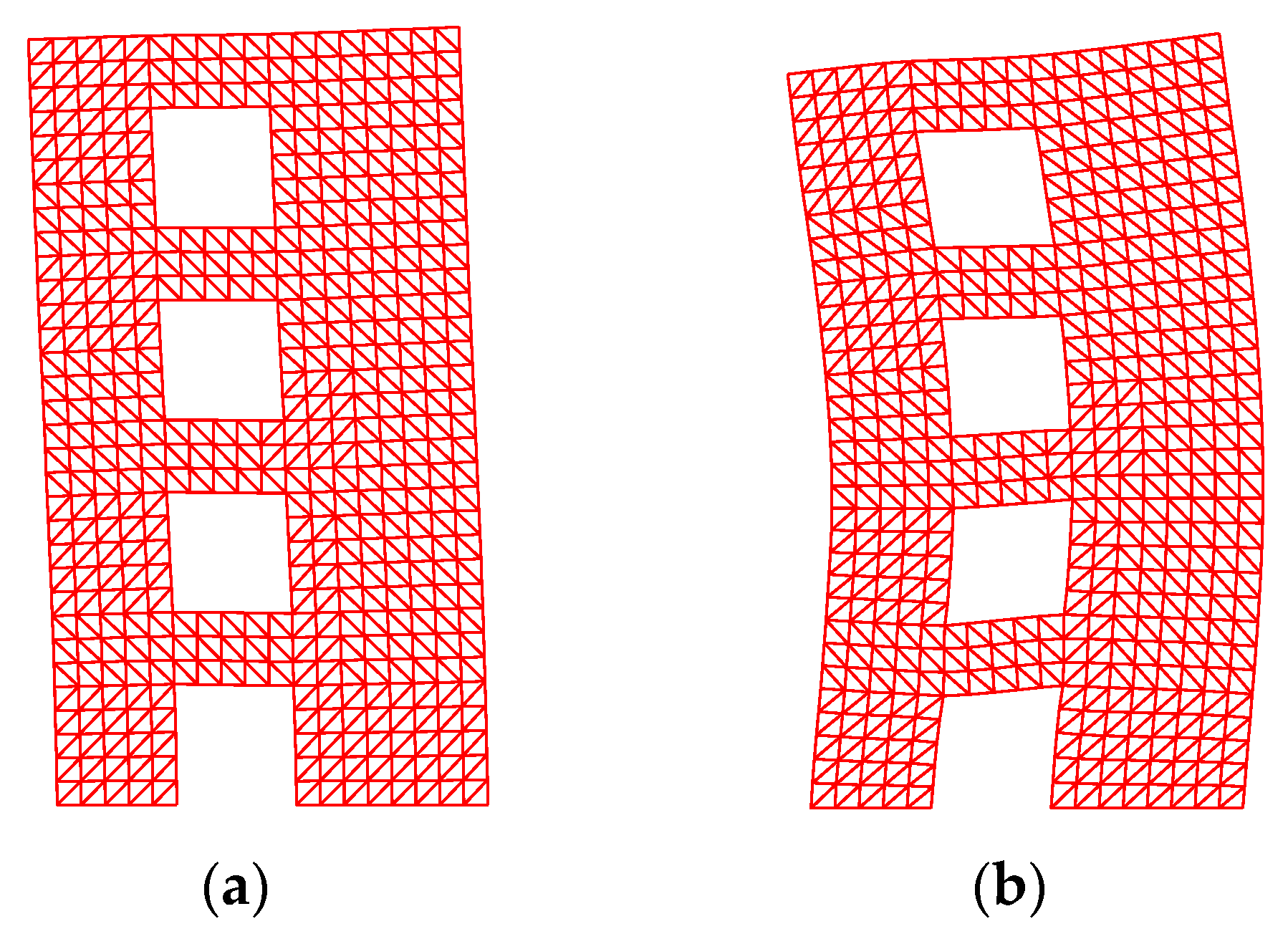
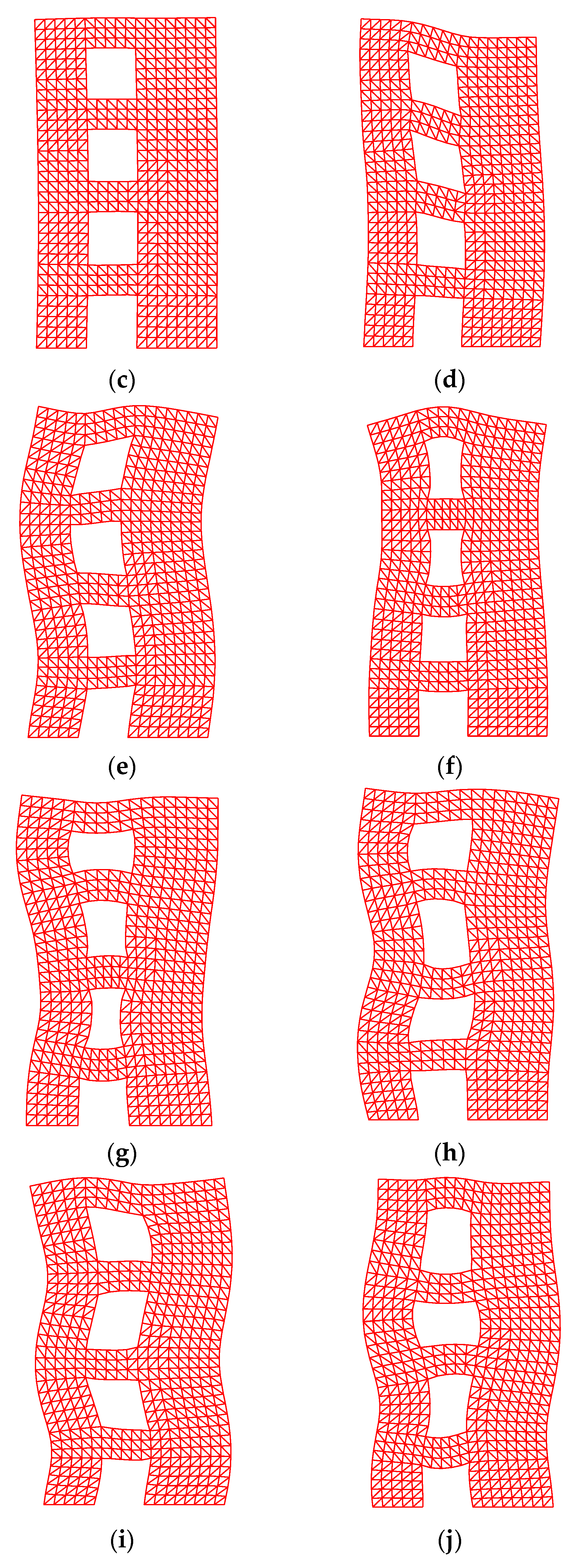
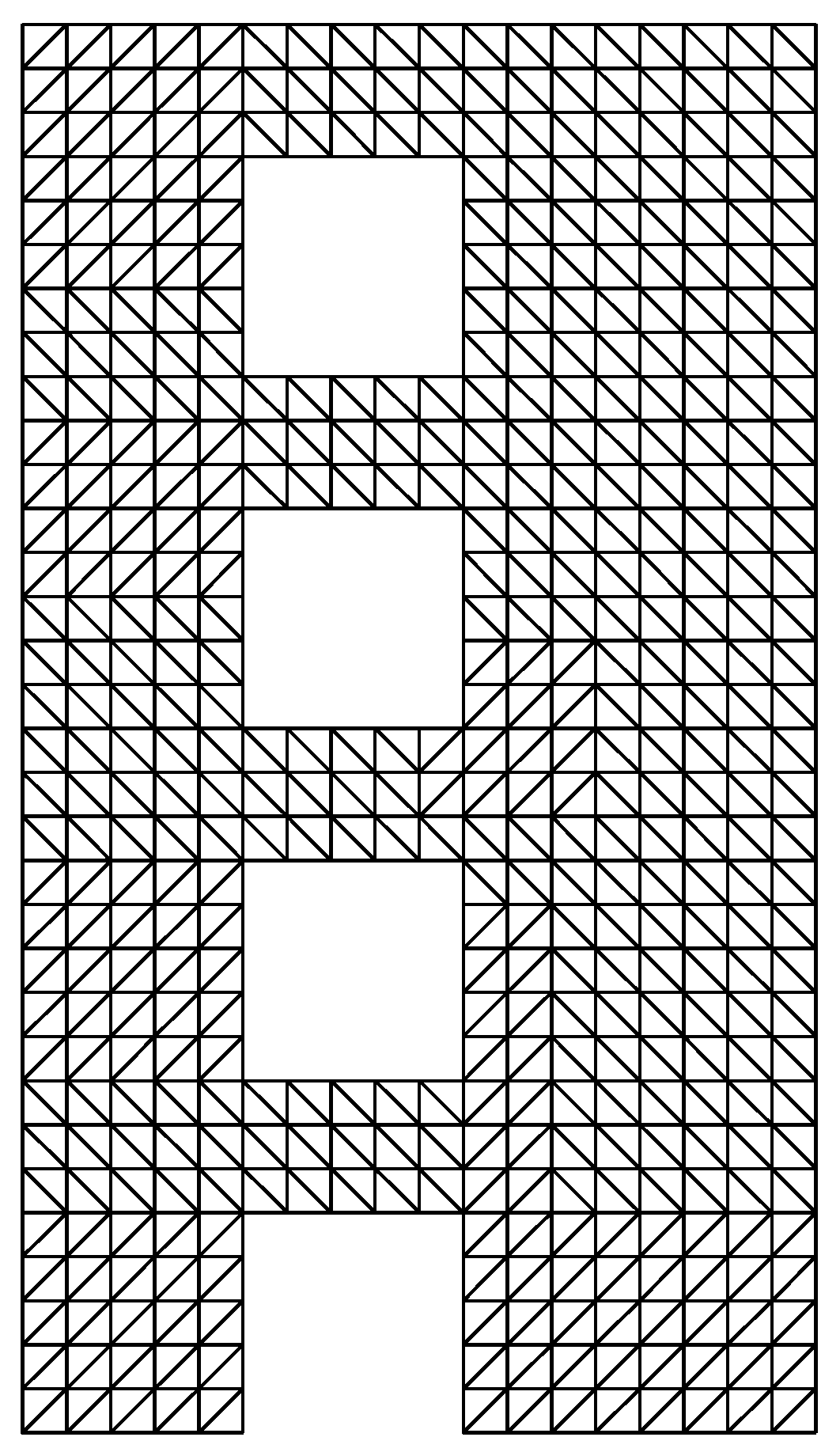
6.2. Free Vibration Analysis of a Shear Wall

The second considered numerical example is a shear wall. As shown in Figure 11, the shear wall has four openings and the fully clamped boundary condition is applied at its bottom edge. The related material constants are mass density $\rho$ = 1, Young’s modulus E = 1000 and Poisson’s ratio v = 0.2. Assuming that this shear wall is in plane stress condition with thickness t = 1. The standard triangular mesh with 952 elements and 599 nodes (see Figure 12) is used in the calculation and

Table 6. The obtained natural frequencies (Hz) results from different elements for the shear wall.

Mode	FEM-T3	FEM-Q4	ES-FEM	EFEM-N3	Reference
1	0.1081	0.1044	0.1032	0.1022	0.1011
2	0.3681	0.3580	0.3553	0.3522	0.3497
3	0.3855	0.3839	0.3836	0.3830	0.3825
4	0.6312	0.6029	0.5916	0.5846	0.5767
5	0.8094	0.7773	0.7677	0.7594	0.7532
6	0.9503	0.9275	0.9214	0.9131	0.9094
7	1.0352	1.0061	0.9983	0.9894	0.9857
8	1.1459	1.1247	1.1158	1.1060	1.1007
9	1.2045	1.1673	1.1552	1.1454	1.1389
10	1.2276	1.1944	1.1844	1.1763	1.1724

lists the computed first 10 natural frequency results from different elements. The reference results are obtained from the commercial software package ABAQUS using very refined triangular meshes (17,136 elements and 17,644 nodes). From the results shown in the table, we can again find that more accurate natural frequency results can be predicted by the present EFEM-N3 than the other mentioned elements. In addition, Figure 13 also gives the first 10 vibration modes from the present EFEM-N3. We can observe that the proposed EFEM-N3 indeed behaves very well in predicting the mode shape in free vibration analysis.

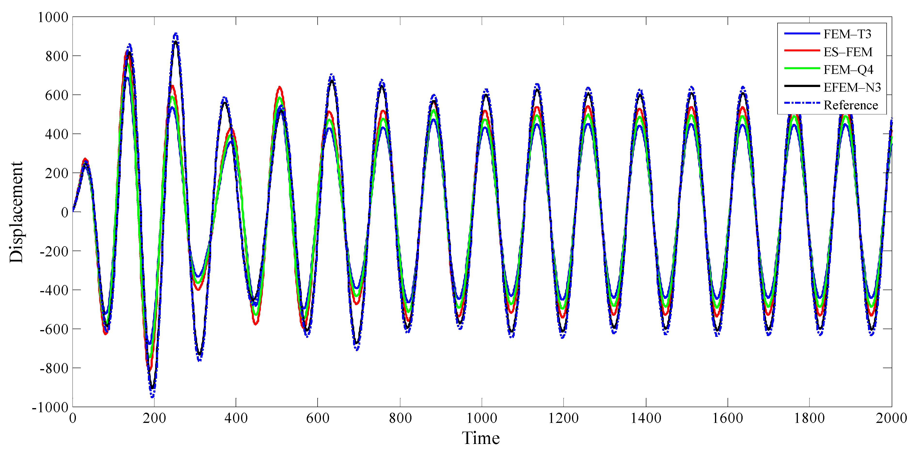
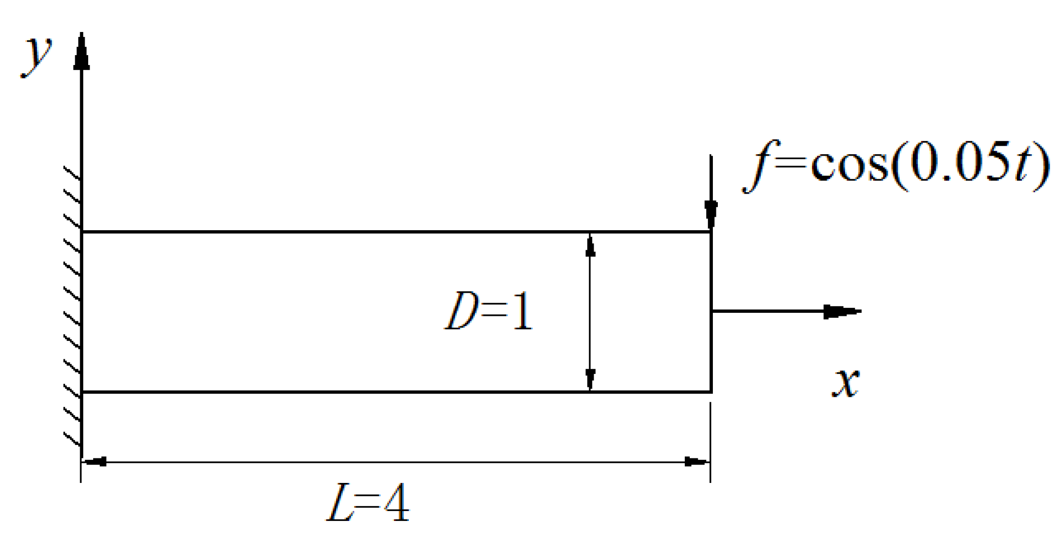
6.3. Forced Vibration Analysis of a Cantilever Beam

A cantilever beam is considered for forced vibration analysis in this section (see Figure 14). The plane stress condition is assumed here and the related material parameters are mass density $\rho$ = 1, Young’s modulus E = 1 and Poisson’s ratio v = 0.3. The Rayleigh damping coefficients are taken as $\alpha$ = 0.005 and $\beta$ = 0.272. A tip harmonic force f = $\cos \left(0.05t\right)$ is subjected to the right end of the cantilever beam in y direction and the Newmark time integration scheme is used for temporal discretization. The uniform mesh pattern with node interval h = 0.2 is employed to discretize the problem domain and the temporal discretization step is $\mathsf{\Delta }t$ = 0.01. Figure 15 shows the transient response results of the right end of the cantilever from different elements. The reference results are from the traditional FEM-Q4 using a very fine mesh (4221 nodes and 4000 elements). From Figure 15, we can observe that all the different numerical methods are able to produce very similar transient response results. However, the EFEM-N3 results are closest to the reference solutions than the other methods. This numerical experiment demonstrates that the proposed EFEM-N3 also behaves very well and can provide better solutions than other methods in dynamic analysis.

7. Conclusions

In this work, a novel linear triangular element enriched by interpolation cover functions (EFEM-N3) is used in tackling the two-dimensional dynamic problems. The following instructive points can be obtained through the considered numerical experiments:

(a)

By employing the proposed scheme in addressing the LD problem in the EFEM-N3, the potential LD issue can be completely removed and then the totally symmetric positive-definite system can be achieved, hence very stable numerical solutions can then be generated.

(b)

Compared to the conventional FEM, the proposed EFEM-N3 in this work behaves much better in convergence rate and computation accuracy, and much more natural frequency results and force response results can be obtained, this is because the initial linear approximation space used in the conventional FEM is effectively enhanced by using the constructed interpolation cover functions.

(c)

Although no extra nodes are needed in the present EFEM-N3 compared to the high order standard elements, more nodal unknowns are involved and larger size system matrices are always obtained, hence the present EFEM-N3 is clearly more numerically expensive. Nevertheless, the present EFEM-N3 still possesses higher computation efficiency in the solution of free and forced vibration analysis.

(d)

The proposed EFEM-N3 is also less sensitive to the mesh distortion than the other conventional elements and quite reliable numerical results can still be produced even if very distorted meshes are employed. Therefore, the present method is very suitable for different areas of engineering applications with complex geometries because the mesh distortion cannot be completely avoided in these cases.

References

1. Zienkiewicz, O.C.; Taylor, R.L. The Finite Element Method, 5th ed.; Butterworth-Heinemann: Oxford, UK, 2000. [Google Scholar]
2. Bathe, K.J. Finite Element Procedures, 2nd ed.; Prentice Hall: Watertown, MA, USA, 2014. [Google Scholar]
3. Chai, Y.B.; Li, W.; Liu, G.R.; Gong, Z.X.; Li, T.Y. A superconvergent alpha finite element method (SαFEM) for static and free vibration analysis of shell structures. Comput. Struct. 2017, 179, 27–47. [Google Scholar] [CrossRef]
4. Chopra, M.B.; Dargush, G.F. Finite-element analysis of time-dependent large-deformation problems. Int. J. Numer. Methods Eng. 1992, 16, 101–130. [Google Scholar] [CrossRef]
5. Moresi, L.; Dufour, F.; Mühlhaus, H.B. A Lagrangian integration point finite element method for large deformation modeling of viscoelastic geomaterials. J. Comput. Phys. 2003, 184, 476–497. [Google Scholar] [CrossRef] [Green Version]
6. Liu, G.R. Mesh Free Methods: Moving Beyond the Finite Element Method; CRC Press: Boca Raton, FL, USA, 2009. [Google Scholar]
7. Belytschko, T.; Lu, Y.Y.; Gu, L. Element-free Galerkin methods. Int. J. Numer. Methods Eng. 1994, 37, 229–256. [Google Scholar] [CrossRef]
8. Chen, J.S.; Hillman, M.; Chi, S.W. Meshfree methods: Progress made after 20 years. J. Eng. Mech. 2017, 143, 04017001. [Google Scholar] [CrossRef] [Green Version]
9. You, X.Y.; Li, W.; Chai, Y.B. A truly meshfree method for solving acoustic problems using local weak form and radial basis functions. Appl. Math. Comput. 2020, 365, 124694. [Google Scholar] [CrossRef]
10. Liu, C.S.; Qiu, L.; Lin, J. Simulating thin plate bending problems by a family of two-parameter homogenization functions. Appl. Math. Model. 2020, 79, 284–299. [Google Scholar] [CrossRef]
11. Li, W.; Zhang, Q.; Gui, Q.; Chai, Y.B. A coupled FE-Meshfree triangular element for acoustic radiation problems. Int. J. Comput. Methods 2021, 18, 2041002. [Google Scholar] [CrossRef]
12. Lin, J.; Zhang, Y.H.; Reutskiy, S.; Feng, W. A novel meshless space-time backward substitution method and its application to nonhomogeneous advection-diffusion problems. Appl. Math. Comput. 2021, 398, 125964. [Google Scholar] [CrossRef]
13. Chai, Y.B.; You, X.Y.; Li, W. Dispersion Reduction for the Wave Propagation Problems Using a Coupled “FE-Meshfree” Triangular Element. Int. J. Comput. Methods 2020, 17, 1950071. [Google Scholar] [CrossRef]
14. Lin, J.; Feng, W.; Reutskiy, S.; Xu, H.; He, Y. A semi-analytical method for solving a class of time fractional partial differential equations with variable coefficients. Appl. Math. Lett. 2021, 112, 106712. [Google Scholar] [CrossRef]
15. Qiu, L.; Lin, J.; Wang, F.J.; Qin, Q.H.; Liu, C.S. A homogenization function method for inverse heat source problems in 3D functionally graded materials. Appl. Math. Model. 2021, 91, 923–933. [Google Scholar] [CrossRef]
16. Wu, T.W. Boundary Element Acoustics: Fundamentals and Computer Codes; WIT Press: Southampton, UK, 2000. [Google Scholar]
17. Gu, Y.; Lei, J. Fracture mechanics analysis of two-dimensional cracked thin structures (from micro- to nano-scales) by an efficient boundary element analysis. Results Math. 2021, 11, 100172. [Google Scholar] [CrossRef]
18. Wang, F.; Fan, C.M.; Zhang, C.; Lin, J. A localized space-time method of fundamental solutions for diffusion and convection-diffusion problems. Adv. Appl. Math. Mech. 2020, 12, 940–958. [Google Scholar] [CrossRef]
19. Li, J.P.; Gu, Y.; Qin, Q.H.; Zhang, L. The rapid assessment for three-dimensional potential model of large-scale particle system by a modified multilevel fast multipole algorithm. Comput. Math. Appl. 2021, 89, 127–138. [Google Scholar] [CrossRef]
20. Li, J.P.; Fu, Z.J.; Gu, Y.; Qin, Q.H. Recent advances and emerging applications of the singular boundary method for large-scale and high-frequency computational acoustics. Adv. Appl. Math. Mech. 2021, 14, 315–343. [Google Scholar] [CrossRef]
21. Fu, Z.J.; Chen, W.; Wen, P.H.; Zhang, C.Z. Singular boundary method for wave propagation analysis in periodic structures. J. Sound Vib. 2018, 425, 170–188. [Google Scholar] [CrossRef]
22. Fu, Z.J.; Xi, Q.; Li, Y.; Huang, H.; Rabczuk, T. Hybrid FEM–SBM solver for structural vibration induced underwater acoustic radiation in shallow marine environment. Comput. Methods Appl. Mech. Eng. 2020, 369, 113236. [Google Scholar] [CrossRef]
23. Li, J.P.; Zhang, L. High-precision calculation of electromagnetic scattering by the Burton-Miller type regularized method of moments. Eng. Anal. Bound. Elem. 2021, 133, 177–184. [Google Scholar] [CrossRef]
24. Li, J.P.; Zhang, L.; Qin, Q.H. A regularized method of moments for three-dimensional time-harmonic electromagnetic scattering. Appl. Math. Lett. 2021, 112, 106746. [Google Scholar] [CrossRef]
25. Gu, Y.; Fan, C.M.; Fu, Z.J. Localized method of fundamental solutions for three-dimensional elasticity problems: Theory. Adv. Appl. Math. Mech. 2021, 13, 1520–1534. [Google Scholar]
26. Liu, W.K.; Jun, S.; Zhang, Y.F. Reproducing kernel particle methods. Int. J. Numer. Methods Fluids 1995, 20, 1081–1106. [Google Scholar] [CrossRef]
27. Nayroles, B.; Touzot, G.; Villon, P. Generalizing the finite element method: Diffuse approximation and diffuse elements. Comput. Mech. 1992, 10, 307–318. [Google Scholar] [CrossRef]
28. Li, X.; Li, S. A fast element-free Galerkin method for the fractional diffusion-wave equation. App. Math. Lett. 2021, 122, 107529. [Google Scholar] [CrossRef]
29. Li, X.; Li, S. A linearized element-free Galerkin method for the complex Ginzburg-Landau equation. Compu. Math. Appl. 2021, 90, 135–147. [Google Scholar] [CrossRef]
30. Harari, I.; Hughes, T.J.R. Galerkin/least-squares finite element methods for the reduced wave equation with non-reflecting boundary conditions in unbounded domains. Comput. Methods Appl. Mech. Eng. 1992, 98, 411–454. [Google Scholar] [CrossRef]
31. Xu, Y.Y.; Zhang, G.Y.; Zhou, B.; Wang, H.Y.; Tang, Q. Analysis of acoustic radiation problems using the cell-based smoothed radial point interpolation method with Dirichlet-to-Neumann boundary condition. Eng. Anal. Bound. Elem. 2019, 108, 447–458. [Google Scholar] [CrossRef]
32. Qu, W.Z.; He, H. A GFDM with supplementary nodes for thin elastic plate bending analysis under dynamic loading. Appl. Math. Lett. 2022, 124, 107664. [Google Scholar] [CrossRef]
33. Qu, W.Z.; Gao, H.W.; Gu, Y. Integrating Krylov deferred correction and generalized finite difference methods for dynamic simulations of wave propagation phenomena in long-time intervals. Adv. Appl. Math. Mech. 2021, 13, 1398–1417. [Google Scholar]
34. Fu, Z.J.; Xie, Z.Y.; Ji, S.Y.; Tsai, C.C.; Li, A.L. Meshless generalized finite difference method for water wave interactions with multiple-bottom-seated-cylinder-array structures. Ocean Eng. 2020, 195, 106736. [Google Scholar] [CrossRef]
35. Oñate, E.; Perazzo, F.; Miquel, J. A finite point method for elasticity problems. Comput. Struct. 2001, 79, 2151–2163. [Google Scholar] [CrossRef]
36. Li, X.; Li, S. A finite point method for the fractional cable equation using meshless smoothed gradients. Eng. Anal. Bound. Elem. 2022, 134, 453–465. [Google Scholar] [CrossRef]
37. Wang, F.; Zhao, Q.; Chen, Z.; Fan, C.M. Localized Chebyshev collocation method for solving elliptic partial differential equations in arbitrary 2D domains. Appl. Math. Comput. 2021, 397, 125903. [Google Scholar] [CrossRef]
38. Xi, Q.; Fu, Z.J.; Zhang, C.Z.; Yin, D.S. An efficient localized Trefftz-based collocation scheme for heat conduction analysis in two kinds of heterogeneous materials under temperature loading. Comput. Struct. 2021, 255, 106619. [Google Scholar] [CrossRef]
39. Xi, Q.; Fu, Z.J.; Wu, W.J.; Wang, H.; Wang, Y. A novel localized collocation solver based on Trefftz basis for Potential-based Inverse Electromyography. Appl. Math. Comput. 2021, 390, 125604. [Google Scholar] [CrossRef]
40. Wang, F.; Wang, C.; Chen, Z.T. Local knot method for 2D and 3D convectiondiffusion-reaction equations in arbitrary domains. Appl. Math. Lett. 2020, 105, 106308. [Google Scholar] [CrossRef]
41. Zeng, W.; Liu, G.R. Smoothed finite element methods (S-FEM): An overview and recent developments. Arch. Comput. Method Eng. 2018, 25, 397–435. [Google Scholar] [CrossRef]
42. Chai, Y.B.; Li, W.; Lei, M.; Liu, G.R. Analysis of coupled structural-acoustic problems based on the smoothed finite element method (S-FEM). Eng. Anal. Bound. Elem. 2014, 42, 84–91. [Google Scholar]
43. Li, W.; Gong, Z.X.; Chai, Y.B.; Cheng, C.; Li, T.Y.; Zhang, Q.F.; Wang, M.S. Hybrid gradient smoothing technique with discrete shear gap method for shell structures. Comput. Math. Appl. 2017, 74, 1826–1855. [Google Scholar] [CrossRef]
44. Chai, Y.B.; Li, W.; Gong, Z.X.; Li, T.Y. Hybrid smoothed finite element method for two dimensional acoustic radiation problems. Appl. Acoust. 2016, 103, 90–101. [Google Scholar] [CrossRef]
45. Chai, Y.B.; Gong, Z.X.; Li, W.; Li, T.Y.; Zhang, Q.F. A smoothed finite element method for exterior Helmholtz equation in two dimensions. Eng. Anal. Bound. Elem. 2017, 84, 237–252. [Google Scholar] [CrossRef]
46. Chai, Y.B.; Li, W.; Gong, Z.X.; Li, T.Y. Hybrid smoothed finite element method for two-dimensional underwater acoustic scattering problems. Ocean Eng. 2016, 116, 129–141. [Google Scholar] [CrossRef]
47. Chai, Y.B.; Gong, Z.X.; Li, W.; Li, T.Y.; Zhang, Q.F.; Zou, Z.H.; Sun, Y.B. Application of smoothed finite element method to two-dimensional exterior problems of acoustic radiation. Int. J. Comput. Methods 2018, 15, 1850029. [Google Scholar] [CrossRef]
48. Jiang, C.; Zhang, Z.Q.; Gao, G.J.; Liu, G.R. A modified immersed smoothed FEM with local field reconstruction for fluid–structure interactions. Eng. Anal. Bound. Elem. 2019, 107, 218–232. [Google Scholar] [CrossRef]
49. Liu, M.Y.; Gao, G.J.; Zhu, H.F.; Jiang, C.; Liu, G.R. A cell-based smoothed finite element method (CS-FEM) for three-dimensional incompressible laminar flows using mixed wedge-hexahedral element. Eng. Anal. Bound. Elem. 2021, 133, 269–285. [Google Scholar] [CrossRef]
50. Chai, Y.B.; You, X.Y.; Li, W.; Huang, Y.; Yue, Z.J.; Wang, M.S. Application of the edge-based gradient smoothing technique to acoustic radiation and acoustic scattering from rigid and elastic structures in two dimensions. Comput. Struct. 2018, 203, 43–58. [Google Scholar] [CrossRef]
51. Li, W.; Chai, Y.B.; Lei, M.; Li, T.Y. Numerical investigation of the edge-based gradient smoothing technique for exterior Helmholtz equation in two dimensions. Comput. Struct. 2017, 182, 149–164. [Google Scholar] [CrossRef]
52. Liu, G.R.; Nguyen-Thoi, T.; Nguyen-Xuan, H.; Lam, K.Y. A node-based smoothed finite element method (NS-FEM) for upper bound solutions to solid mechanics problems. Comput. Struct. 2009, 87, 14–26. [Google Scholar] [CrossRef]
53. Chai, Y.B.; Li, W.; Li, T.Y.; Gong, Z.X.; You, X.Y. Analysis of underwater acoustic scattering problems using stable node-based smoothed finite element method. Eng. Anal. Bound. Elem. 2016, 72, 27–41. [Google Scholar] [CrossRef]
54. Ham, S.; Bathe, K.J. A finite element method enriched for wave propagation problems. Comput. Struct. 2012, 94, 1–12. [Google Scholar] [CrossRef] [Green Version]
55. Chai, Y.B.; Bathe, K.J. Transient wave propagation in inhomogeneous media with enriched overlapping triangular elements. Comput. Struct. 2020, 237, 106273. [Google Scholar] [CrossRef]
56. Kim, J.; Bathe, K.J. The finite element method enriched by interpolation covers. Comput. Struct. 2013, 116, 35–49. [Google Scholar] [CrossRef]
57. Kim, J.; Bathe, K.J. Towards a procedure to automatically improve finite element solutions by interpolation covers. Comput. Struct. 2014, 131, 81–97. [Google Scholar] [CrossRef]
58. Chai, Y.B.; Li, W.; Liu, Z.Y. Analysis of transient wave propagation dynamics using the enriched finite element method with interpolation cover functions. Appl. Math. Comput. 2022, 412, 126564. [Google Scholar] [CrossRef]
59. Gui, Q.; Zhou, Y.; Li, W.; Chai, Y.B. Analysis of two-dimensional acoustic radiation problems using the finite element with cover functions. Appl. Acoust. 2022, 185, 108408. [Google Scholar] [CrossRef]
60. Wu, F.; Zhou, G.; Gu, Q.Y.; Chai, Y.B. An enriched finite element method with interpolation cover functions for acoustic analysis in high frequencies. Eng. Anal. Bound. Elem. 2021, 129, 67–81. [Google Scholar] [CrossRef]
61. Jeon, H.M.; Lee, P.S.; Bathe, K.J. The MITC3 shell finite element enriched by interpolation covers. Comput. Struct. 2014, 134, 128–142. [Google Scholar] [CrossRef]
62. Jun, H.; Yoon, K.; Lee, P.S.; Bathe, K.J. The MITC3+ shell element enriched in membrane displacements by interpolation covers. Comput. Methods Appl. Mech. Eng. 2018, 337, 58–80. [Google Scholar] [CrossRef]
63. Liu, G.R.; Gu, Y.T. A local radial point interpolation method (LRPIM) for free vibration analyses of 2-D solids. J. Sound Vib. 2001, 246, 29–46. [Google Scholar] [CrossRef] [Green Version]
64. Dai, K.Y.; Liu, G.R. Free and forced vibration analysis using the smoothed finite element method (SFEM). J. Sound Vib. 2007, 301, 803–820. [Google Scholar] [CrossRef]
Figure 1. The illustration of the linear triangular element enriched with interpolation cover functions: (a) The original linear shape functions; (b) The cover region of the interpolation cover functions; (c) The overlapping domain of the cover regions.
Mathematics 10 00456 g001
Figure 2. The employed coordinate system in the EFEM formulation: (a) The local coordinates and physical coordinates; (b) The natural coordinate system.
Mathematics 10 00456 g002
Figure 3. The nine shape functions for one triangular element in the EFEM formulation.
Mathematics 10 00456 g003
Figure 4. The illustration of the imposition of Dirichlet boundary condition.
Mathematics 10 00456 g004
Figure 5. A two-dimensional cantilever beam.
Mathematics 10 00456 g005
Figure 6. The standard triangular mesh with regular node distribution for the cantilever beam. (a) Mesh 1 (10 × 1); (b) Mesh 2 (20 × 2); (c) Mesh 3 (40 × 4).
Mathematics 10 00456 g006
Figure 7. The first 10 vibration modes of cantilever beam calculated by EFEM-N3: (a) Mode one; (b) Mode Two; (c) Mode Three; (d) Mode Four; (e) Mode Five; (f) Mode six; (g) Mode Seven; (h) Mode Eight; (i) Mode Nine; (j) Mode Ten.
Mathematics 10 00456 g007aMathematics 10 00456 g007b
Figure 8. Comparison of the convergence properties of various methods in calculating the natural frequencies of the cantilever beam. (a) Mode 1, (b) Mode 2.
Mathematics 10 00456 g008aMathematics 10 00456 g008b
Figure 9. Comparison of the computation efficiency of the different elements. (a) Mode 1, (b) Mode 2.
Mathematics 10 00456 g009
Figure 10. Two distorted meshes obtained from the uniform mesh using different irregularity indicators. (a) The irregularity indicator β i r = 0.25, (b) The irregularity indicator β i r = 0.45.
Mathematics 10 00456 g010
Figure 11. A shear wall in plane stress condition for free vibration analysis.
Mathematics 10 00456 g011
Figure 12. The standard triangular mesh for the shear wall.
Mathematics 10 00456 g012
Figure 13. The first 10 vibration modes for the share wall from EFEM-N3: (a) Mode one; (b) Mode Two; (c) Mode Three; (d) Mode Four; (e) Mode Five; (f) Mode six; (g) Mode Seven; (h) Mode Eight; (i) Mode Nine; (j) Mode Ten.
Mathematics 10 00456 g013aMathematics 10 00456 g013b
Figure 14. The cantilever beam under a time-harmonic load.
Mathematics 10 00456 g014
Figure 15. Comparison of transient displacement solutions for the cantilever beam by EFEM-N3.
Mathematics 10 00456 g015