Article

Stability and Numerical Solutions of Second Wave Mathematical Modeling on COVID-19 and Omicron Outbreak Strategy of Pandemic: Analytical and Error Analysis of Approximate Series Solutions by Using HPM

1
School of Computing Science and Engineering, VIT Bhopal University, Bhopal-Indore Highway, Sehore 466114, India
2
Department of Mathematics, Bharath Institute of Higher Education and Research, Chennai 600073, India
3
College of Science and Engineering, Hamad Bin Khalifa University, Doha 602024, Qatar
4
College of Information Sciences and Technology, Data Science and Artificial Intelligence Program, Penn State University, State College, PA 16801, USA
5
School of Optometry and Vision Science, Faculty of Science, Department of Chemical Engineering, University of Waterloo, 200 University Ave W, Waterloo, ON N2L 3G1, Canada
6
Faculty of Engineering, University of Waterloo, 200 University Ave W, Waterloo, ON N2L 3G1, Canada
7
Department of Information Technology, College of Computers and Information Technology, Taif University, P.O. Box 11099, Taif 21944, Saudi Arabia
8
Department of Computer Science and Engineering, University of New South Wales, Sydney 56890, Australia
*
Authors to whom correspondence should be addressed.
Mathematics 2022, 10(3), 343; https://doi.org/10.3390/math10030343
Submission received: 10 December 2021 / Revised: 10 January 2022 / Accepted: 17 January 2022 / Published: 24 January 2022
(This article belongs to the Special Issue Epidemic Models: Track and Control)

Abstract

:
This paper deals with the mathematical modeling of the second wave of COVID-19 and verifies the current Omicron variant pandemic data in India. We also we discussed such as uniformly bounded of the system, Equilibrium analysis and basic reproduction number R 0 . We calculated the analytic solutions by HPM (homotopy perturbation method) and used Mathematica 12 software for numerical analysis up to 8th order approximation. It checked the error values of the approximation while the system has residual error, absolute error and h curve initial derivation of square error at up to 8th order approximation. The basic reproduction number ranges between 0.8454 and 2.0317 to form numerical simulation, it helps to identify the whole system fluctuations. Finally, our proposed model validated (from real life data) the highly affected five states of COVID-19 and the Omicron variant. The algorithm guidelines are used for international arrivals, with Omicron variant cases updated by the Union Health Ministry in January 2022. Right now, the third wave is underway in India, and we conclude that it may peak by the end of May 2022.

1. Introduction

COVID-19 spread is increasing in urban areas across India and Omicron cases are also increasing. In December 2021, Omicron is the leading variants compare to other variants. So for, each state has increased the cases of Omicron spread. Now COVID-19 active cases were increased in India and it is very soon end for this pandemic. COVID-19 cases in India as of 30 December 2021, collected from the WHO (World Health Organization) is as follows: via passengers screened at the airport (1,524,266), active cases (82,402), cured or discharged (34,258,778), deaths (480,860), total active cases (160,989), last total cured (33,614,434), last total death (456386), and total samples tested (605,885,769). The total vaccination doses as of the current date is 1,438,322,742.
The Omicron variant of COVID-19 has been detected in 653 cases across India by Union Health Ministry data updated in December 2021. As of 30 December 2021, COVID-19 cases are increasing in India. On 29 December 2021, there were 13187 new cases identified, a 77% increase from the previous week. Cases are surging in other states such as Mumbai, Delhi, Pune, Bengaluru, Chennai, Thane, Kolkata and Ahmedabad. Mumbai identified 2510 cases on 29 December 2021; this was an 80% increase from the previous day and 400% rise from a week previous. Similarly, Delhi identified 923 cases (600% rise), Bengaluru 400 cases (90%), Chennai 294 (100%), Mumbai (15%), etc. The current high rate is due to the Omicron variant. It is a type of the SARS-CoV-2 virus and dominant in India in the last few days of December 2021. The percentage of vaccination is 63% of its adults and 89% of partial in India.
Even though there are some vaccinations and medicines for control this pandemic treated at COVID-19 gives a big challenge to the people. Moreover, we discuss equilibrium points of COVID-19 to lessen the infected individuals in India. We have given the convergent, comparable and most appropriate solution of each and every compartment involved in the model by using the most powerful and elegant method via the homotopy perturbaton method. Particularly in India, it has decided lots of control strategy polices followed by peoples, due to quarantine period measures such as lock down, social distances, speed up of treatment, wearing mask, sanitizer usages and frequently wash hands are respectively [1,2,3,4,5,6,7].
Chakraborty T, Ghosh I. [8], discuss the real life data and dangerous assessment of COVID-19 by using data-driven analysis. The analysis of prediction of COVID-19 spreads are in China, Italy and France in [9]. The isolation of cases and contacts are to control COVID-19 outbreaks [10]. We collected the Indian data separately in the Indian council of medical research (ICMR) [11]. Dynamics and bifurcation approaches are defined in [12]. Kucharski AJ et al. [13], it gives a spread model study on transmission and infected data on COVID-19. The R 0 of COVID-19 is calculated and data fluctuations to other viruses [14,15]. Ndariou F, et al. [16], the COVID-19 model in Wuhan which is considered and control strategies in [17] with similar to Brazil [18]. The mathematical modelling of the improved SIR model with real life government control strategies [19] with SARSCoV-2 in India [20]. We collected the tracker data from crowd sourcing in India [21]. SEIR is a good model which enables the COVID-19 outbreak in all countries with government polices and other endemic models for source data [22,23,24,25]. M. A. Khan, A. Atangana [26], A Mathematical Modeling of novel Corona-virus (2019-nCoV) is studied with numerical simulation and asymptomatic carrier transmission [27]. The compartment models are defined by [28] with phase based [29]. The numerical data’s are in all countries, we used this procedure the calculations [30,31,32]. It helps to all the analysis such as control in Wuhan, China [33,34]. The Indian dynamics are of transmission and control strategy are derived from the mathematical modeling [35] with New dynamical behavior in [36]. In this regard, we calculated the active cases from the mathematical modeling and then created a new model in the second wave with the Omicron variant. We obtained the infected ratio for the period October 2021 to December 2021 and the parameter estimation of the model. The described model is solved numerically as well as approximated analytically by using the homotopy perturbation method.
In general, we collected all data from the WHO [37] with optimal control theories [38,39,40]. The supporting data collected from other government recongnised websites [41,42,43,44]. The four states (Kerala, Sikkim, Mizoram and Meghalaya) are an exception to the endemic state (they are not yet endemic). It will soon change and become endemic. Almost the majority of population is infected state. The affected population had 68 percentage (nearly 1000 million) antibodies from 4th ICMR survey by end of December 2021. The cumulative COVID-19 cases had 30,410,577 (3.2 percentage out of affected population).
Finally, we concluded that the five highly affected states of Maharashtra, kerala, Karnataka, Tamilnadu and Andra Pradesh need more attention to decrease the spread to the infected populations. The number of people infected with COVID-19 was still high in many areas, and transmission of the virus was easily regenerated once people increased their activities and contact with each other. The current pandemic situation is to reduce the infection of COVID-19 cases in India. Scientists are currently working to find opt vaccine for corona virus disease from various countries.
This research paper is written as follows: In 
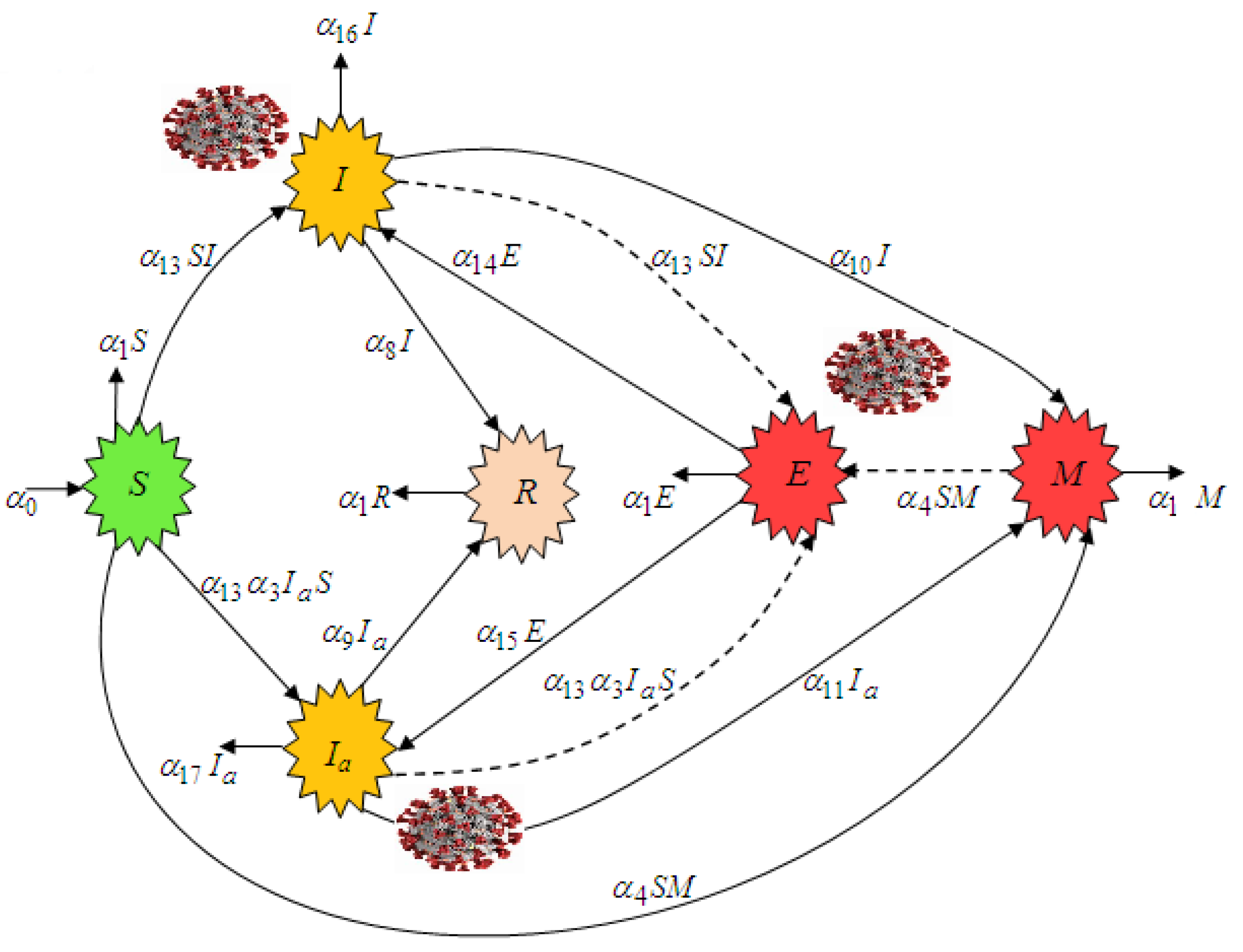
Section 2, we have given the detailed mathematical modeling of the second wave of the Indian COVID-19 pandemic. In Section 3, Stability analysis of the model like uniformly bounded of the system, equilibrium analysis such as disease free equilibrium and endemic free equilibrium and basic reproduction number is studied.
In Section 4 and Section 5, the approximate analytical expressions of each and every compartment appeared in the given model are derived using HPM. Also, we briefly discuss the numerical analysis and error analysis for the Section 6 and Section 7. The concluding remarks are provided in Section 7.

2. Mathematical Modelling of Second Wave COVID-19

In the Indian perspective, the analysis of different strategies on COVID-19 transmission dynamics in the presence of different intervention schemes becomes significant. Considering the significant role of intervention strategies, there are many researchers that have obtained a new epidemic model with different intervention strategies of COVID-19 in a homogeneous host population. The appearance and recurrence of coronavirus are epidemics modeling researchers to model. The proposed model all parameters details are given by Table 1. Let us define the compartmental mathematical model (epidemic model) that has been developed by Kham and Atangana [26] for understanding the transmission of the virus and some interesting in Figure 1 (see also [16,27,32,37]).
In this epidemic model a total number of populations N at a time t, is divided into the following six compartments:
The system of nonlinear ordinary differential equations representing this epidemic model is as follows:
d S d t = α 0 α 1 S α 2 S ( I + α 3 I a ) N α 4 S M d E d t = α 2 S ( I + α 3 I a ) N + α 4 S M ( 1 α 5 ) α 6 E α 5 α 7 E α 1 E d I d t = ( 1 α 5 ) α 6 E ( α 8 + α 1 ) I d I a d t = α 5 α 7 E ( α 9 + α 1 ) I a d R d t = α 8 I + α 9 I a α 1 R d M d t = α 10 I + α 11 I a α 1 M
To understand the above system of Equation (1) more clearly, we rewrite the same system in the following way by substituting some more constants as follows:
d S d t = α 0 α 1 S α 13 S ( I + α 3 I a ) α 4 S M d E d t = α 13 S ( I + α 3 I a ) + α 4 S M α 14 E α 15 E α 1 E d I d t = α 14 E α 16 I d I a d t = α 15 E α 17 I a d R d t = α 8 I + α 9 I a α 1 R d M d t = α 10 I + α 11 I a α 1 M
where
α 13 = α 2 N , α 14 = ( 1 α 5 ) α 6 , α 15 = α 5 α 7 , α 16 = α 8 + α 1 and α 17 = α 9 + α 1
with the initial conditions for finding the solution of Equation (2) are
S ( 0 ) = S 0 , E ( 0 ) = E 0 , I ( 0 ) = I 0 , I a ( 0 ) = I a 0 , R ( 0 ) = R 0 and M ( 0 ) = M 0

3. Stability Analysis of Second Wave COVID-19

3.1. Uniformly Bounded of The System

In this section, we produced uniformly boundedness of the system. It analyzed the initial values of the system with boundary of positivity, and identified the region of the system of equations. Let
X = S + E + I + I a + R + M d X d t = d S d t + d E d t + d I d t + d I a d t + d R d t + d M d t d X d t = α 0 α 1 X + α 10 I + α 11 I a d X d t + α 1 X α 0 , t . Region = X R + 6 : 0 X ( S , E , I , I a , R , M ) < α 0 α 1 + ε , ε > 0 .

3.2. Equilibrium Analysis of COVID-19

This section is very important role in mathematical model while the systems analysis to get the disturbances of the boundary. It makes to find the solutions either stable or unstable with stability of whole system of equations. The study on equilibrium of COVID-19 deals with several things such as the equilibrium on the regional economies of a country, the equilibrium at the population level. It is calculated to derive the disease free and endemic equilibrium points. These two cases the derivative is equal to zero.
α 0 α 1 S α 13 S ( I + α 3 I a ) α 4 S M = 0 α 13 S ( I + α 3 I a ) + α 4 S M α 14 E α 15 E α 1 E = 0 α 14 E α 16 I = 0 α 15 E α 17 I a = 0 α 8 I + α 9 I a α 1 R = 0 α 10 I + α 11 I a α 1 M = 0
Then we solved the equilibrium points of S, E, I, I a , R and M.

3.3. Disease Free Equilibrium for COVID-19

The current scenario spread is low or not affected the infection such cases only exposed and infection classes must be zero. In this case, we got the susceptible solutions and remaining all are zero. This case there is no infection of COVID-19. We put E = I = I a = 0 .
The disease free equilibrium points are:
S = α 0 α 1 , E = 0 , I = 0 , I a = 0 , R = 0 , M = 0

3.4. Endemic Equilibrium for COVID-19

It is used to find the spread of COVID-19 infection. This case all compartments are not equal to zero. We have found the calculations of spread and all fluctuations clearly identified. It is very useful for whole boundary. The endemic equilibrium points are:
S = α 1 α 16 α 17 α 14 + α 15 + α 1 α 14 α 17 ( α 4 α 10 + α 13 α 1 ) + α 15 α 16 ( α 4 α 11 + α 13 α 3 α 1 ) E = α 0 ( α 4 α 10 + α 13 α 1 ) α 14 α 17 + α 15 α 16 ( α 4 α 11 + α 13 α 1 α 3 ) α 1 α 16 α 17 α 1 ( α 14 + α 15 + α 1 ) ( α 14 + α 15 + α 1 ) [ α 4 ( α 10 α 14 α 17 + α 11 α 15 α 16 ) + α 13 ( α 14 α 17 α 1 + α 15 α 3 α 16 α 1 ) ] I = α 14 α 1 α 16 α 17 α 1 ( α 14 + α 15 + α 1 ) + α 0 α 4 ( α 14 α 10 α 17 + α 11 α 15 α 16 ) + α 0 α 13 ( α 14 α 17 α 1 α 15 α 3 α 16 α 1 α 16 [ ( α 14 + α 15 + α 1 ) ( α 4 ( α 10 α 14 α 17 + α 11 α 15 α 16 ) + α 13 ( α 14 α 17 α 1 + α 15 α 3 α 16 α 1 ) ] I a = α 15 [ α 1 α 16 α 17 α 1 ( α 14 + α 15 + α 1 ) α 0 α 4 ( α 10 α 14 α 17 α 11 α 15 α 16 ) α 0 α 13 α 1 ( α 14 α 17 α 15 α 3 α 16 ) ] α 17 ( α 14 + α 15 + α 1 ) α 4 α 14 ( α 10 α 17 + 1 ) + α 1 α 13 ( α 14 α 17 + α 15 α 3 α 16 R = ( ( α 1 α 16 α 17 α 1 ( α 14 α 15 + α 1 ) α 0 α 4 ( α 10 α 14 α 17 + α 11 α 15 α 16 ) α 0 α 1 α 13 ( α 14 α 17 α 15 α 3 ) ) ( α 8 α 14 α 17 + α 9 α 15 α 16 ) ) α 1 α 16 α 17 ( α 14 + α 15 + α 1 ) [ α 4 ( α 10 α 17 + α 11 α 15 α 16 ) + α 1 α 13 ( α 14 α 17 + α 15 α 3 α 16 ) ] M = ( ( α 1 α 16 α 17 α 1 ( α 14 + α 15 + α 1 ) α 0 α 4 ( α 10 α 14 α 17 + α 11 α 15 α 16 α 0 α 1 α 13 ( α 14 α 17 + α 15 α 3 α 16 ) ) ( α 10 α 14 α 17 + α 11 α 15 α 16 ) ) ) ( ( α 14 + α 15 + α 1 ) ( α 4 ( α 10 α 14 α 17 + α 11 α 15 α 16 ) + α 1 α 13 ( α 14 α 17 α 1 + α 15 α 3 α 16 α 1 ) ( α 1 α 16 α 17 ) ) )
we calculate the Jacobian matix
J = α 1 0 α 13 s α 3 s 0 α 4 s 0 ( α 14 + α 15 + α 1 ) α 13 s α 3 s 0 α 4 s 0 α 14 α 16 0 0 0 0 α 15 0 α 17 0 0 0 0 α 8 α 9 α 1 0 0 0 α 10 α 11 0 α 1
Then to find the eigen values of the above matrix
λ I J = λ + α 1 0 α 13 s α 3 s 0 α 4 s 0 λ + α 14 + α 15 + α 1 α 13 s α 3 s 0 α 4 s 0 α 14 λ + α 16 0 0 0 0 α 15 0 λ + α 17 0 0 0 0 α 8 α 9 λ + α 1 0 0 0 α 10 α 11 0 λ + α 1 = 0 a 0 λ 6 + a 1 λ 5 + a 2 λ 4 + a 3 λ 3 + a 4 λ 2 + a 5 λ + a 6 = 0
a 0 = 1 , a 1 = ( 4 α 1 + α 14 + α 15 + α 17 + α 16 ) , a 2 = ( α 14 α 17 + 2 α 16 α 1 + α 16 ( α 15 + α 14 + α 17 ) + α 14 α 1 + α 17 α 1 + α 16 α 1 + 2 α 17 α 1 + α 1 2 + 2 α 1 α 1 α 14 α 13 s + α 15 α 1 + α 15 α 1 + α 15 α 17 + α 14 α 1 α 15 α 13 α 3 s α 1 ( α 14 2 α 1 α 15 α 1 α 17 α 16 ) ) , a 3 = ( α 1 2 ( α 16 + α 17 + α 1 ) α 15 α 13 α 3 s ( α 1 α 1 ) + α 15 α 16 α 1 α 14 α 13 s α 1 + α 15 α 11 α 4 s α 14 α 13 s α 1 + α 14 α 10 α 4 s α 14 α 13 s α 17 α 1 ( α 14 α 17 α 16 ( 2 α 1 + α 15 + α 14 + α 17 + α 1 ) α 1 ( α 14 + 2 α 17 + α 1 + 2 α 1 ) + α 14 α 13 s α 15 ( α 1 + α 1 + α 17 α 13 α 3 s ) α 1 ( α 14 + α 17 ) ) + α 14 α 1 α 1 + α 15 α 17 α 1 + α 15 α 17 α 1 + α 14 α 17 α 1 + 2 α 17 α 1 2 + α 15 α 16 α 1 + α 14 α 16 α 17 + α 14 α 17 α 1 + α 16 α 17 α 1 + 2 α 16 α 1 2 + α 15 α 1 2 + α 14 α 16 α 1 + α 14 α 16 α 1 α 15 α 16 α 13 α 3 s + α 15 α 16 α 17 + 2 α 16 α 17 α 1 ) , a 4 = ( α 14 α 16 α 1 2 + α 14 α 16 α 17 α 1 + α 15 α 16 α 17 α 1 + α 14 α 10 α 4 s α 1 α 14 α 13 s α 1 2 + α 14 α 10 α 4 s α 17 α 14 α 13 s α 17 α 1 + α 17 α 1 2 α 12 + α 17 α 15 α 1 2 + α 15 α 16 α 1 2 + α 15 α 16 α 11 α 4 s + α 16 α 1 2 α 17 + α 14 α 17 α 1 2 + α 15 α 16 α 17 α 1 + α 16 α 1 3 + α 15 α 11 α 4 s α 1 α 15 α 16 α 13 α 3 s α 1 α 14 α 13 α 17 s α 1 + α 14 α 16 α 17 α 1 α 15 α 16 α 13 α 3 s α 1 + 2 α 16 α 17 α 1 2 α 15 α 13 α 3 s α 1 2 α 1 ( α 1 2 α 16 α 17 α 1 2 α 1 3 + α 15 α 13 α 3 s α 1 + α 15 α 13 α 3 s α 1 α 15 α 16 α 1 + α 14 α 13 s α 1 α 15 α 11 α 4 s + α 14 α 13 s α 1 α 14 α 10 α 4 s + α 14 α 13 s α 17 α 14 α 1 2 α 15 α 17 α 1 α 15 α 17 α 1 α 14 α 12 α 17 2 α 17 α 1 2 α 15 α 16 α 1 α 14 α 16 α 17 α 14 α 17 α 1 α 17 α 16 α 1 2 α 16 α 1 2 α 15 α 1 α 14 α 16 α 1 α 14 α 16 α 1 + α 15 α 16 α 13 α 3 s α 15 α 16 α 17 2 α 16 α 17 α 1 ) ) , a 5 = ( α 1 ( α 14 α 16 α 1 2 α 14 α 16 α 17 α 1 α 15 α 16 α 17 α 1 α 14 α 10 α 4 s α 1 + α 14 α 13 s α 1 2 α 14 α 10 α 4 s α 17 + α 14 α 13 s α 17 α 1 α 17 α 1 3 α 15 α 17 α 1 2 α 15 α 16 α 1 2 α 15 α 16 α 11 α 4 s α 17 α 1 2 α 16 α 14 α 17 α 1 2 α 15 α 16 α 17 α 1 α 16 α 1 3 α 15 α 11 α 4 s α 1 + α 15 α 16 α 13 α 3 s α 1 + α 14 α 13 s α 17 α 1 α 14 α 16 α 17 α 1 + α 15 α 16 α 13 α 3 s α 1 2 α 16 α 17 α 1 2 + α 15 α 13 α 3 s α 1 2 ) + α 15 α 16 α 11 α 4 s α 1 + α 14 α 10 α 4 s α 17 α 1 + α 15 α 16 α 17 α 1 2 + α 14 α 16 α 17 α 1 2 α 14 α 13 s α 17 α 1 2 + α 1 2 α 16 α 17 α 1 α 15 α 16 α 13 α 3 s α 1 2 ) , a 6 = α 1 ( α 15 α 16 α 11 α 4 s α 1 α 14 α 10 α 4 s α 17 α 1 α 15 α 16 α 17 α 1 2 α 14 α 16 α 17 α 1 2 + α 14 α 13 s α 17 α 1 2 α 1 3 α 16 α 17 + α 15 α 16 α 13 α 3 s α 1 2 ) .
We changed the above characteristic equation by using Descartes’ rule of sign as follows:
a 0 λ 6 a 1 λ 5 + a 2 λ 4 a 3 λ 3 + a 4 λ 2 a 5 λ + a 6 = 0 ,
with conditions a 0 , a 1 , a 2 , a 3 , a 4 , a 5 , a 6 > 0 & λ 1 , λ 2 , λ 3 , λ 4 , λ 5 , λ 6 < 0 .
The eigen values are negative, the equilibrium point is globally asymptotic stable.

3.5. The Basic Reproduction Number R 0

The system of equations all nature fluctuations are controlled by R 0 and either greater or less than compare to one. The control parameter R 0 is the model validation with nature of disease spread when compare to real life data. This section we used by next generation matrix method as defined:
F = 0 α 13 s α 13 α 3 s α 4 s α 14 0 0 0 α 15 0 0 0 0 α 10 α 11 0 V 1 = 1 α 14 + α 15 + α 1 α 14 α 16 ( α 14 + α 15 + α 1 ) α 14 α 17 ( α 14 + α 15 + α 1 ) 0 0 1 α 16 0 0 0 0 1 α 17 0 0 0 0 1 α 1 P = F V 1 = 0 α 13 s α 16 α 13 α 3 s α 17 α 4 s α 1 α 14 α 14 + α 15 + α 1 α 14 2 α 16 ( α 14 + α 15 + α 1 ) α 14 α 15 α 17 ( α 14 + α 15 + α 1 ) 0 α 15 α 14 + α 15 + α 1 α 14 α 15 α 16 ( α 14 + α 15 + α 1 ) α 15 2 α 17 ( α 14 + α 15 + α 1 ) 0 0 α 10 α 16 α 11 α 17 0 R 0 = 2 α 4 α 15 2 α 10 α 14 α 0 α 1 2 α 16 α 17 ( α 14 + α 15 + α 1 ) 2

4. Homotopy Perturbation Method (HPM) Procedure for COVID-19 Model

It is a good method to find the analytic solutions for the system of nonlinear differential equations with convergence solutions of the derivation in the series solutions. The first two terms are enough to get the convergence solutions of zeroth order deformation at approximations. The series solutions are to get the error analysis up to maximum in mathematical modeling of nonlinear ODE. Let us consider the given equation is converted to below form:
(1-p) (linear terms of given differential equations) + p (linear and nonlinear all terms of given differential equations) = 0.
Let us organized the given model all variables as follows:
S ( t ) = S 0 + p S 1 + p 2 S 2 + . . . + . E ( t ) = E 0 + p E 1 + p 2 E 2 + . . . + . I ( t ) = I 0 + p I 1 + p 2 I 2 + . . . + . I a ( t ) = I a 0 + p I a 1 + p 2 I a 2 + . . . + . R ( t ) = R 0 + p R 1 + p 2 R 2 + . . . + . M ( t ) = M 0 + p M 1 + p 2 M 2 + . . . + .
Approximate solutions of COVID-19 are:
S ( t ) = lim p 1 S ( t ) = S 0 + S 1 + S 2 + . . . + . E ( t ) = lim p 1 E ( t ) = E 0 + E 1 + E 2 + . . . + . I ( t ) = lim p 1 I ( t ) = I 0 + I 1 + I 2 + . . . + . I a ( t ) = lim p 1 I a ( t ) = I a 0 + I a 1 + I a 2 + . . . + . R ( t ) = lim p 1 R ( t ) = R 0 + R 1 + R 2 + . . . + . M ( t ) = lim p 1 M ( t ) = M 0 + M 1 + M 2 + . . . + .
Here the first two terms are enough to get the approximate analytic solutions of converges of numerical simulations. This method is very helpful for solving nonlinear ordinary differential equations.

5. Application of HPM in COVID-19 Model

The solution of the system of Equation (2) can be obtained by using HPM as follows:
d S d t = α 0 α 1 S α 13 S ( I + α 3 I a ) α 4 S M
d E d t = α 13 S ( I + α 3 I a ) + α 4 S M α 14 E α 15 E α 1 E
d I d t = α 14 E α 16 I
d I a d t = α 15 E α 17 I a
d R d t = α 8 I + α 9 I a α 1 R
d M d t = α 10 I + α 11 I a α 1 M
To obtain the analytical solution, we construct the homotopy as follows:
( 1 p ) d S d t α 0 + α 1 S + p d S d t α 0 + α 1 S + α 13 S ( I + α 3 I a ) + α 4 S M = 0 ( 1 p ) d E d t + ( α 14 + α 15 + α 1 ) E
+ p d E d t + ( α 14 + α 15 + α 1 ) E α 13 S ( I + α 3 I a ) + α 4 S M = 0
( 1 p ) d I d t + α 16 I + p d I d t + α 16 I α 14 E = 0
( 1 p ) d I a d t + α 17 I a + p d I a d t + α 17 I a + α 15 E = 0
( 1 p ) d R d t + α 1 R + p d R d t + α 1 R α 8 I α 9 I a = 0
( 1 p ) d M d t + α 1 M + p d M d t + α 12 M α 10 I α 11 I a = 0
Equating p 0 terms on both sides of the above system of Equations (11)–(16), we get constructing homotopy, we get
p 0 : d S 0 d t = α 0 α 1 S 0
p 0 : d E 0 d t = α 14 E 0 α 15 E 0 α 1 E 0
p 0 : d I 0 d t = α 16 I 0
p 0 : d I a 0 d t = α 17 I a 0
p 0 : d R 0 d t = α 1 R 0
p 0 : d M 0 d t = α 1 M 0
The solution for these equations are given as follows
S 0 = α 0 α 1 + c 1 e α 1 t
E 0 = c 2 e ( α 14 + α 15 + α 1 ) t
I 0 = c 3 e α 16 t
I a 0 = c 4 e α 17 t
R 0 = c 5 e α 1 t
M 0 = c 6 e α 1 t
Applying initial conditions,
S ( 0 ) = β 0 ; E ( 0 ) = β 1 ; I ( 0 ) = β 2 ; I a ( 0 ) = β 3 ; R ( 0 ) = β 4 ; M ( 0 ) = β 5 ,
for all β i > 0 , i = 0 , 1 , 2 , 3 , 4 , 5 and initial approximations,
S ( i ) = 0 ; E ( i ) = 0 ; I ( i ) = 0 ; I a ( i ) = 0 ; R ( i ) = 0 ; M ( i ) = 0 for all i = 1 , 2 , 3 . . .
By applying Equation (29) into Equation (23), we get
c 1 = β 0 α 0 α 1
Therefore
S 0 = α 0 α 1 + β 0 α 0 α 1 e α 1 t
Similarly by applying Equation (29) into Equations (24)–(28), we get
c 2 = β 1
E 0 = β 1 e E 0 ( α 14 + α 15 + α 1 ) t
c 3 = β 2
I 0 = β 2 e α 16 t
c 4 = β 3
I a 0 = β 3 e α 17 t
c 5 = β 4
R 0 = β 4 e α 1 t
c 6 = β 5
M 0 = β 5 e α 1 t
Again equating p 1 terms, we get
p 1 : d S 1 d t = α 0 α 1 S 1 α 13 S 0 I 0 α 13 α 3 S 0 I a 0 α 4 S 0 M 0
p 1 : d E 1 d t = α 13 S 0 I 0 + α 13 α 3 S 0 I a 0 + α 4 S 0 M 0 α 14 E 1 α 15 E 1 α 1 E 1
p 1 : d I 1 d t = α 14 E 0 α 16 I 1
p 1 : d I a 1 d t = α 15 E 0 α 17 I a 1
p 1 : d R 1 d t = α 8 I 0 + α 9 I a 0 α 1 R 1
p 1 : d M 1 d t = α 10 I 0 + α 11 I a 0 α 1 M 1
From Equation (43) ⇒
d S 1 d t = α 0 α 1 S 1 α 13 α 0 α 1 + β 0 α 0 α 1 exp ( α 1 t ) β 2 exp ( α 16 t ) α 13 α 3 α 0 α 1 + β 0 α 0 α 1 exp ( α 1 t ) β 3 exp ( α 17 t ) α 4 α 0 α 1 + β 0 α 0 α 1 exp ( α 1 t ) β 5 exp ( α 1 t ) S 1 = α 0 α 1 + α 13 β 2 α 16 + α 1 α 0 α 1 1 α 16 α 13 β 0 α 0 α 1 + α 13 α 3 β 3 α 17 + α 1 α 0 α 1 1 α 17 α 13 α 3 β 0 α 0 α 1 + α 4 β 5 α 2 + α 1 α 0 α 1 1 α 1 α 4 β 0 α 0 α 1 e α 1 t + α 0 α 1 α 13 β 2 α 16 + α 1 α 0 α 1 e α 16 t + α 13 β 2 α 16 β 0 α 0 α 1 e ( α 1 + α 16 ) t α 13 α 3 β 3 α 1 α 17 α 0 α 1 e α 17 t + α 13 α 3 β 3 α 17 β 0 α 0 α 1 e ( α 1 + α 17 ) t α 4 β 5 α 1 α 2 α 0 α 1 e α 12 t + β 3 α 1 β 0 α 0 α 1 e ( 2 α 1 ) t
d E 1 d t = α 13 α 0 α 1 + β 0 α 0 α 1 exp ( α 1 t ) β 2 exp ( α 16 t ) + α 13 α 3 α 0 α 1 + β 0 α 0 α 1 exp ( α 1 t ) β 3 exp ( α 17 t ) + α 4 α 0 α 1 + β 0 α 0 α 1 exp ( α 1 t ) β 5 exp ( α 1 t ) α 14 E 1 α 15 E 1 α 1 E E 1 = 1 α 16 + ( α 14 + α 15 + α 1 ) α 13 α 0 α 1 β 2 1 ( α 1 + α 16 ) + ( α 14 + α 15 + α 1 ) α 13 β 0 α 0 α 1 1 α 17 + ( α 14 + α 15 + α 1 ) α 13 α 3 α 0 α 1 β 3 1 ( α 1 + α 17 ) + ( α 14 + α 15 + α 1 ) α 13 α 3 β 0 α 0 α 1 1 α 1 + ( α 14 + α 15 + α 1 ) α 4 α 0 α 1 β 5 1 ( 2 α 1 ) + ( α 14 + α 15 + α 1 ) α 4 β 0 α 0 α 1 exp ( ( α 14 + α 15 + α 1 ) t ) + 1 α 16 + ( α 14 + α 15 + α 1 ) α 13 α 0 α 1 β 2 exp ( α 16 t ) + 1 ( α 1 + α 16 ) + ( α 14 + α 15 + α 1 ) α 13 β 0 α 0 α 1 exp ( α 1 t ) β 2 exp ( α 16 t ) + 1 α 17 + ( α 14 + α 15 + α 1 ) α 13 α 3 α 0 α 1 β 3 exp ( α 17 t ) + 1 ( α 1 + α 17 ) + ( α 14 + α 15 + α 1 ) α 13 α 3 β 0 α 0 α 1 exp ( α 1 t ) β 3 exp ( α 17 t ) + 1 α 1 + ( α 14 + α 15 + α 1 ) α 4 α 0 α 1 β 5 exp ( α 1 t )
+ 1 ( 2 α 1 ) + ( α 14 + α 15 + α 1 ) α 4 β 0 α 0 α 1 exp ( α 1 t ) β 3 exp ( α 1 t ) I 1 = c 9 exp ( α 16 t ) + 1 ( α 14 + α 15 + α 1 ) + α 16 α 14 β 1 exp ( ( α 14 + α 15 + α 1 ) t )
Applying initial condition I ( 0 ) = 0
c 9 + 1 ( α 14 + α 15 + α 1 ) + α 16 α 14 β 1 = 0 I 1 = 1 ( α 14 + α 15 + α 1 ) + α 16 α 14 β 1 exp ( α 16 t ) + 1 ( α 14 + α 15 + α 1 ) + α 16 α 14 β 1 exp ( ( α 14 + α 15 + α 1 ) t ) d I 1 d t = α 14 β 1 exp ( ( α 14 + α 15 + α 1 ) t ) α 16 I 1 d I a 1 d t = α 15 β 1 exp ( ( α 14 + α 15 + α 1 ) t ) α 17 I a 1 I a 1 = c 10 exp ( α 17 t ) + 1 ( α 14 + α 15 + α 1 ) + α 17 α 15 β 1 exp ( ( α 14 + α 15 + α 1 ) t )
Applying initial condition I a ( 0 ) = 0
c 10 + 1 ( α 14 + α 15 + α 1 ) + α 17 α 15 β 1 = 0 I a 1 = 1 ( α 14 + α 15 + α 1 ) + α 17 α 15 β 1 exp ( α 17 t ) + 1 ( α 14 + α 15 + α 1 ) + α 17 α 15 β 1 exp ( ( α 14 + α 15 + α 1 ) t ) d R 1 d t = α 8 β 2 exp ( α 16 t ) + α 9 β 3 exp ( α 17 t ) α 1 R 1 R 1 = c 11 exp ( α 1 t ) + 1 α 16 + α 1 α 8 β 2 exp ( α 16 t ) + 1 α 17 + α 1 α 9 β 3 exp ( α 17 t )
Applying initial condition
R ( 0 ) = 0 c 11 + 1 α 16 + α 1 α 8 β 2 + 1 α 17 + α 1 α 9 β 3 = 0 R 1 = 1 α 16 + α 1 α 8 β 2 1 α 17 + α 1 α 9 β 3 exp ( α 1 t ) + 1 α 16 + α 1 α 8 β 2 exp ( α 16 t ) + 1 α 17 + α 1 α 9 β 3 exp ( α 17 t ) d M 1 d t = α 10 β 2 exp ( α 16 t ) + α 11 β 3 exp ( α 17 t ) α 1 M 1
M 1 = c 12 exp ( α 1 t ) + 1 α 16 + α 1 α 10 β 2 exp ( α 16 t ) + 1 α 17 + α 1 α 11 β 3 exp ( α 17 t )
Applying initial condition
M ( 0 ) = 0 c 12 + 1 α 16 + α 1 α 10 β 2 + 1 α 17 + α 1 α 11 β 3 = 0 M 1 = 1 α 16 + α 1 α 10 β 2 1 α 17 + α 1 α 11 β 3 exp ( α 1 t ) + 1 α 16 + α 1 α 10 β 2 exp ( α 16 t ) + 1 α 17 + α 1 α 11 β 3 exp ( α 17 t )

6. Numerical Analysis

This section plays very big role in modeling. It is the validation of the system of equations from real life data. The initial values and parameters are calculated from data as per government reconsigned websites.
After substitution for all parameters, we got the 8th order approximation and error estimation. Therefore, analytical solutions are verified from comparative study of numerical experiments with the help of software. The numerical solutions are possible to get all types of nonlinear ODE. We consider the parameter values as follows [41,42,43,44]:
N = 6 , 757 , 131 , S 0 = 6 , 757 , 131 , E 0 = 20 , 000 , I 0 = 104 , 591 , I a 0 = 200 , R 0 = 5 , 744 , 693 , M 0 = 907 , 883 , α 0 = 50 , α 1 = 1 76.79 × 365 = 0.0000356 , α 2 = 0.05 , α 3 = 0.02 , α 4 = 0.000001231 , α 5 = 0.1243 , α 6 = 0.00047876 , α 7 = 0.005 , α 8 = 0.09871 , α 9 = 0.854302 , α 10 = 0.000398 , α 11 = 0.001 , α 12 = 0.01 , α 14 = 1 α 5 α 6 = 0.000419 , α 15 = α 5 α 7 = 0.000622 , α 16 = α 8 + α 1 = 0.098745678 , α 17 = α 9 + α 1 = 0.85433768
Let us use Mathematica 12 software to obtain 8th order approximation: S t , E t ,...... M t .
S ( t ) = 9 , 065 , 518 + 6 , 151 , 989 h t + 2 , 648 , 092 h 2 t + 451 , 983 h 3 t + 66 , 467 h 4 t + 6258 h 5 t + 878 h 6 t + 71 h 7 t + 65 h 8 t + 55 h 2 t 2 + 53 h 3 t 2 + 43 h 4 t 2 + 39 h 5 t 2 + 27 h 6 t 2 + 22 h 7 t 2 + 17 h 8 t 2 + . . . , E ( t ) = 300 , 000 + 480 , 795 h t + 371 , 138 h 2 t + 77 , 144 h 3 t + 18 , 273 h 4 t + 2853 h 5 t + 355 h 6 t + 36 h 7 t + 33 h 8 t + 30 h 2 t 2 + 26 h 3 t 2 + 22 h 4 t 2 + 19 h 5 t 2 + 17 h 6 t 2 + 15 h 7 t 2 + 9 h 8 t 2 + . . . , I ( t ) = 280 + 115 h t + 110 h 2 t + 99 h 3 t + 83 h 4 t + 79 h 5 t + 76 h 6 t + 75 h 7 t + 71 h 8 t + 67 h 2 t 2 + 63 h 3 t 2 + 59 h 4 t 2 + 44 h 5 t 2 + 39 h 6 t 2 + 33 h 7 t 2 + 21 h 8 t 2 + . . . , I a ( t ) = 199 + 190 h t + 173 h 2 t + 151 h 3 t + 143 h 4 t + 137 h 5 t + 129 h 6 t + 119 h 7 t + 115 h 8 t + 101 h 2 t 2 + 91 h 3 t 2 + 83 h 4 t 2 + 77 h 5 t 2 + 65 h 6 t 2 + 52 h 7 t 2 + 41 h 8 t 2 + . . . , R ( t ) = 197 + 190 h t + 167 h 2 t + 150 h 3 t + 143 h 4 t + 133 h 5 t + 123 h 6 t + 111 h 7 t + 109 h 8 t + 99 h 2 t 2 + 87 h 3 t 2 + 85 h 4 t 2 + 77 h 5 t 2 + 64 h 6 t 2 + 53 h 7 t 2 + 41 h 8 t 2 + . . . , M ( t ) = 60 , 000 + 190 h t + 183 h 2 t + 177 h 3 t + 165 h 4 t + 157 h 5 t + 147 h 6 t + 133 h 7 t + 129 h 8 t + 119 h 2 t 2 + 107 h 3 t 2 + 96 h 4 t 2 + 88 h 5 t 2 + 71 h 6 t 2 + 67 h 7 t 2 + 55 h 8 t 2 + . . . ,

7. Error Analysis

In this section, it is an important role in series solutions with numerical calculations and an error analysis is produced to obtain the optimal values of parameters. Table 2 shows the h value ranges for each compartment. It controls the series solution approximations at all system of equations and optimal solutions of each compartment in Table 3. Hence, it is to find the estimated h * values in all compartments and also calculated the residual errors for E R 1 , E R 2 , E R 3 E R 4 , E R 5 and E R 6 in Table 4 at time period 0 to 1. The another case is square residual error with each derivative is zero, the we calculated the h * values. The following error residuals are organized as follows:
E R 1 S ; h 1 = d φ S t , h 1 d t = α 0 α 1 s t , h 1 α B s t , h 1 I t , h 1 + I a t , h 1 α 3 α 4 S t , h 1 M t , h 1 E R 2 E ; h 2 = d ϕ E t , h 2 d t = α 13 S t , h 2 I t , h 2 + I a t , h 2 α 3 + α 4 S t , h 2 M t , h 2 α 14 E t , h 2 α 13 E t , h 2 α 1 t , h 2 E R 3 I ; h 3 = d ϕ I t , h 3 d t = α 14 E t , h 3 α 16 I t , h 3 E R 4 I a ; h 4 = d ϕ I a t , h 4 d t = α 15 E t , h 4 α 17 I a t , h 4 E R 5 R ; h 5 = d ϕ R t , h 5 d t = α 8 I t , h 5 + α 9 I a t , h 5 α 1 R t , h 5 E R 6 M ; h 6 = d ϕ M t , h 6 d t = α 10 I t , h 6 + α 11 I a t , h 6 α 12 M t , h 6
Let us consider the square residual error for 8th order approximation:
S ( h 1 ) = 0 1 E R 1 S , E , I , I a , R , M ; h 1 2 d t , E ( h 2 ) = 0 1 E R 2 S , E , I , I a , R , M ; h 2 2 d t , I ( h 3 ) = 0 1 E R 3 S , E , I , I a , R , M ; h 3 2 d t , I a ( h 1 ) = 0 1 E R 4 S , E , I , I a , R , M ; h 4 2 d t , R ( h 5 ) = 0 1 E R 5 S , E , I , I a , R , M ; h 5 2 d t , M ( h 6 ) = 0 1 E R 6 S , E , I , I a , R , M ; h 6 2 d t ,
The minimal values of R X h 1 , R Y h 2 , R V h 3 and R Z h 4 are shown:
d S ( h 1 * ) d h 1 = 0 , d E ( h 2 * ) d h 2 = 0 , d I ( h 3 * ) d h 3 = 0 , d I a ( h 4 * ) d h 4 = 0 . d R ( h 5 * ) d h 5 = 0 . d M ( h 6 * ) d h 6 = 0 .
We consider the optimal values of h 1 * , h 2 * , h 3 * , h 4 * , h 5 * and h 6 * for all of the cases are
h 1 * = 1.1 , h 2 * = 1.2 , h 3 * = 1.3 , h 4 * = 1.4 , h 5 * = 1.5 , h 6 * = 1.6 .
There are three types of errors that are calculated from the numerical experiment. It is very useful for accuracy of exact solutions and numerical simulations. The residual error of 8th order approximation is defined for E R 1 , E R 2 , E R 3 , E R 4 , E R 5 and E R 6 in Figure 2. The absolute error of 8th order approximation is defined for E R 1 , E R 2 , E R 3 , E R 4 , E R 5 and E R 6 in Figure 3. The h curves initial derivatives of 7th and 8th order approximation is calculated from HPM in Figure 4. The square residual error of 8th order approximation is derived in Figure 5. Numerical simulation of ranges of reproduction numbers are R 0 = 2.0317; 1.2922; 1.4809; 1.5972; 0.9844; 0.8454. in Figure 6. It gives the fluctuations of the overall model validation.

8. End of Second Wave Validity Checking

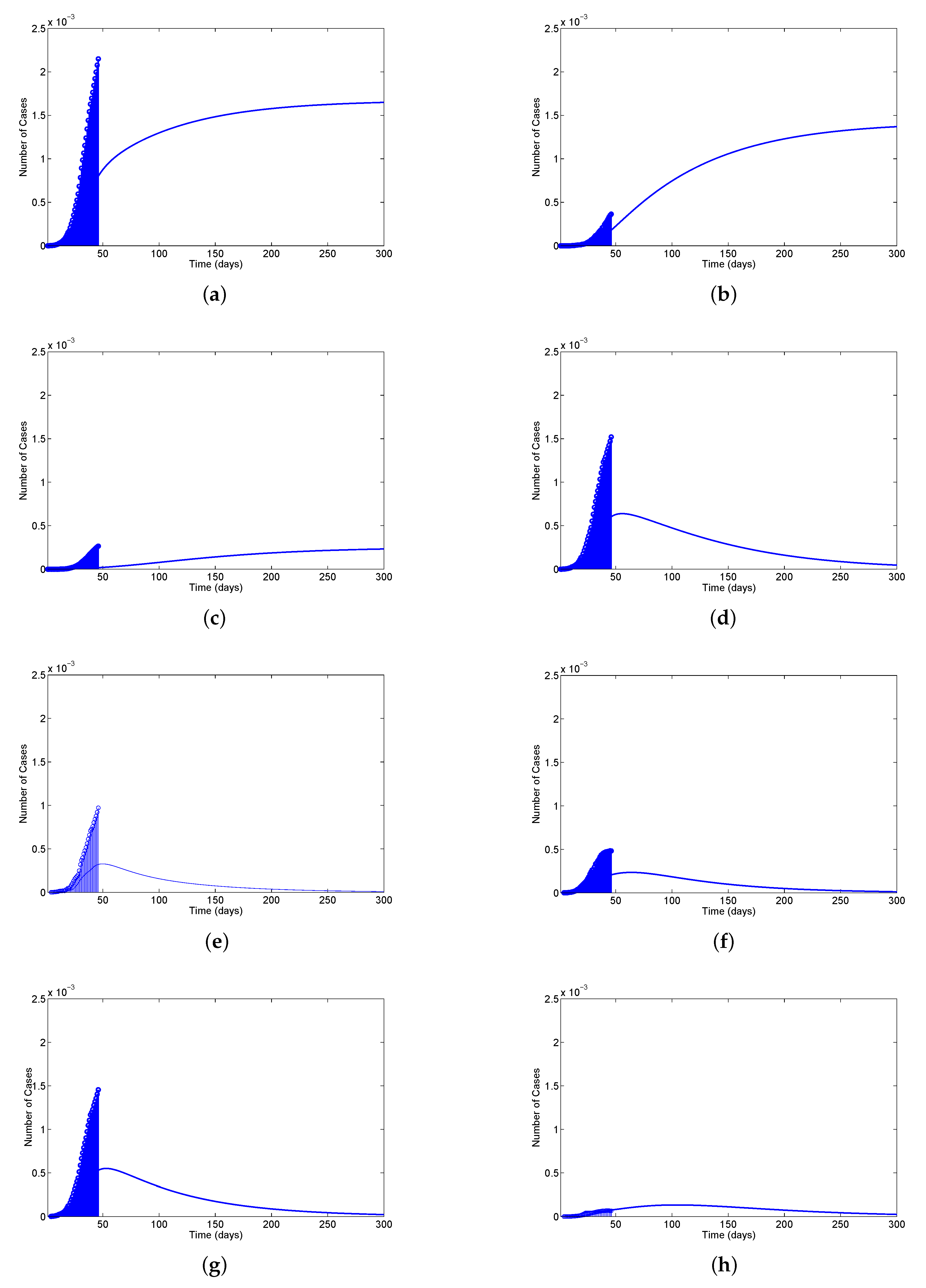
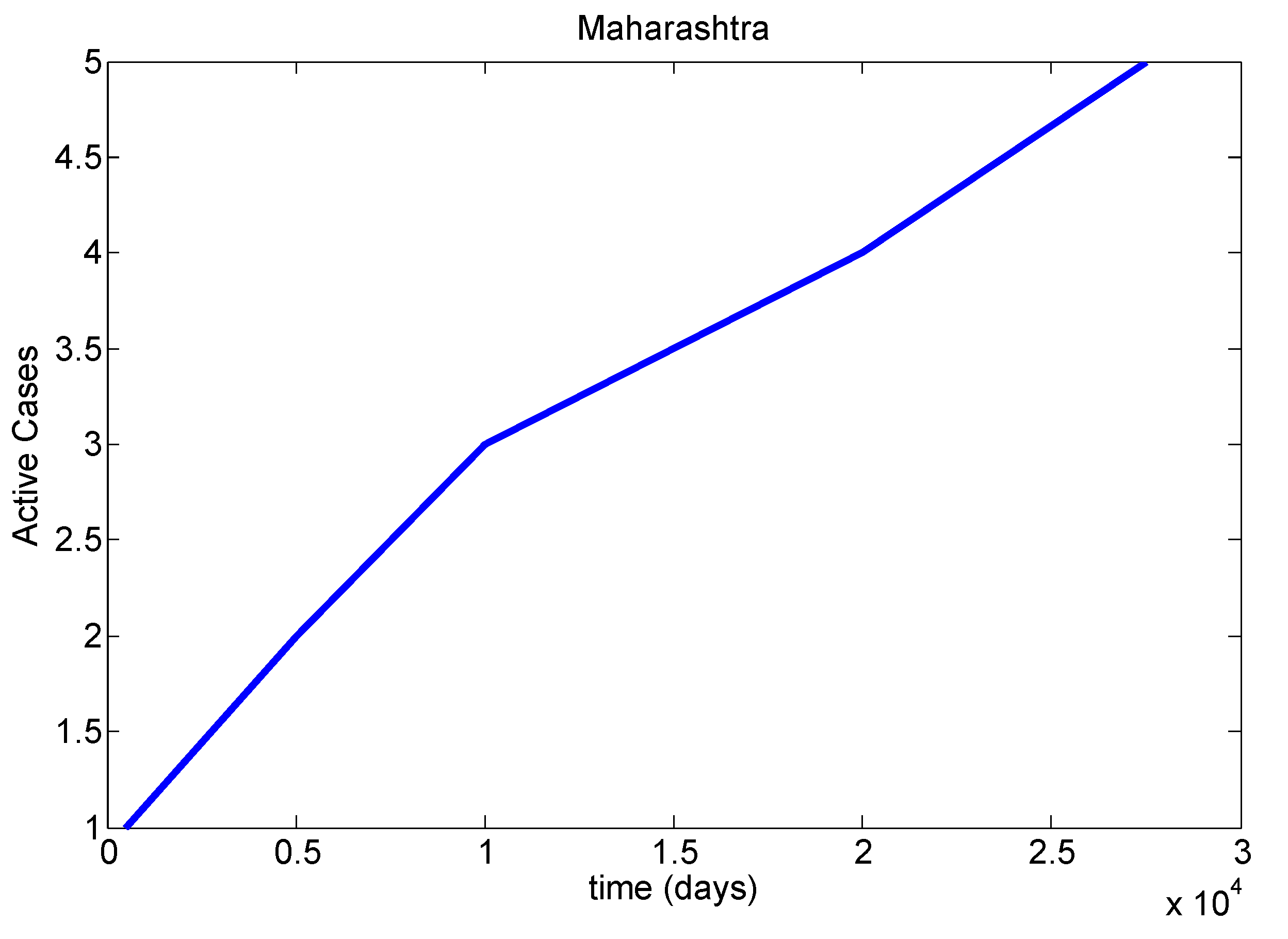
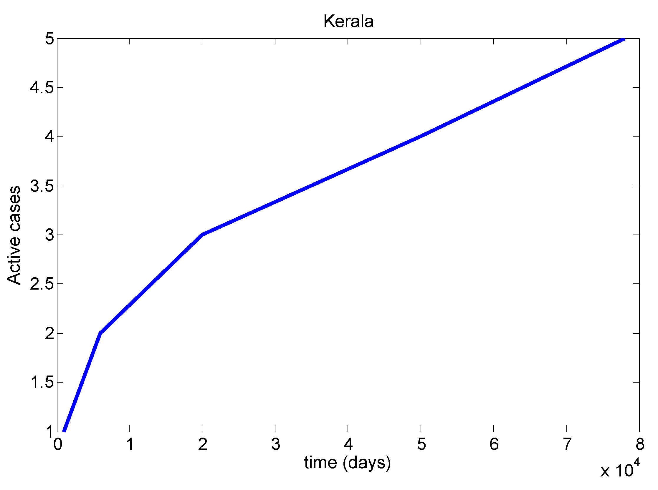
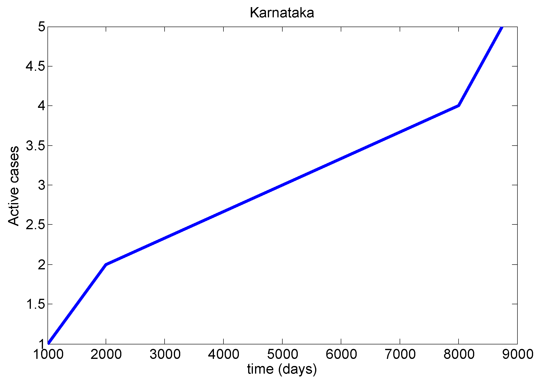
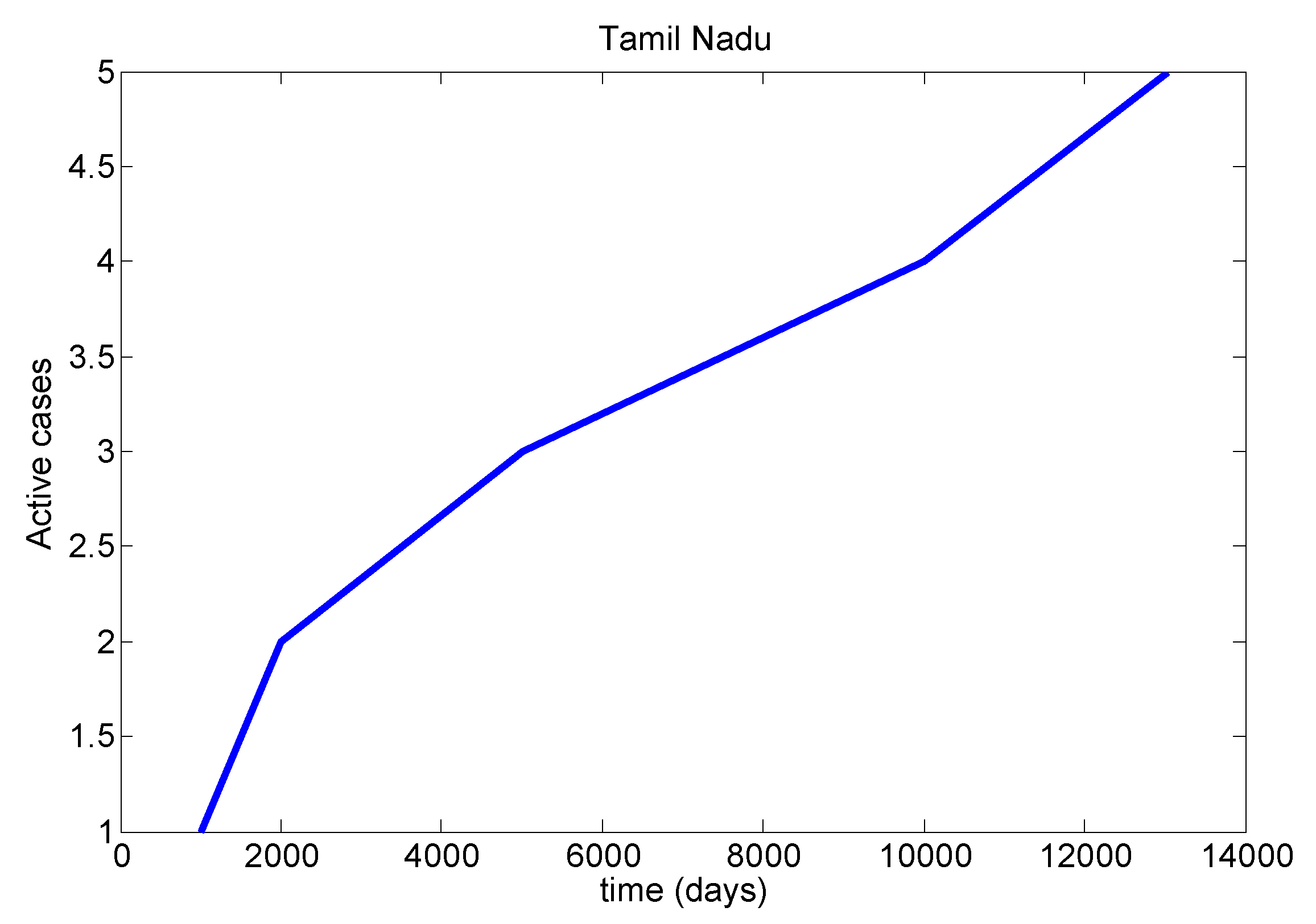
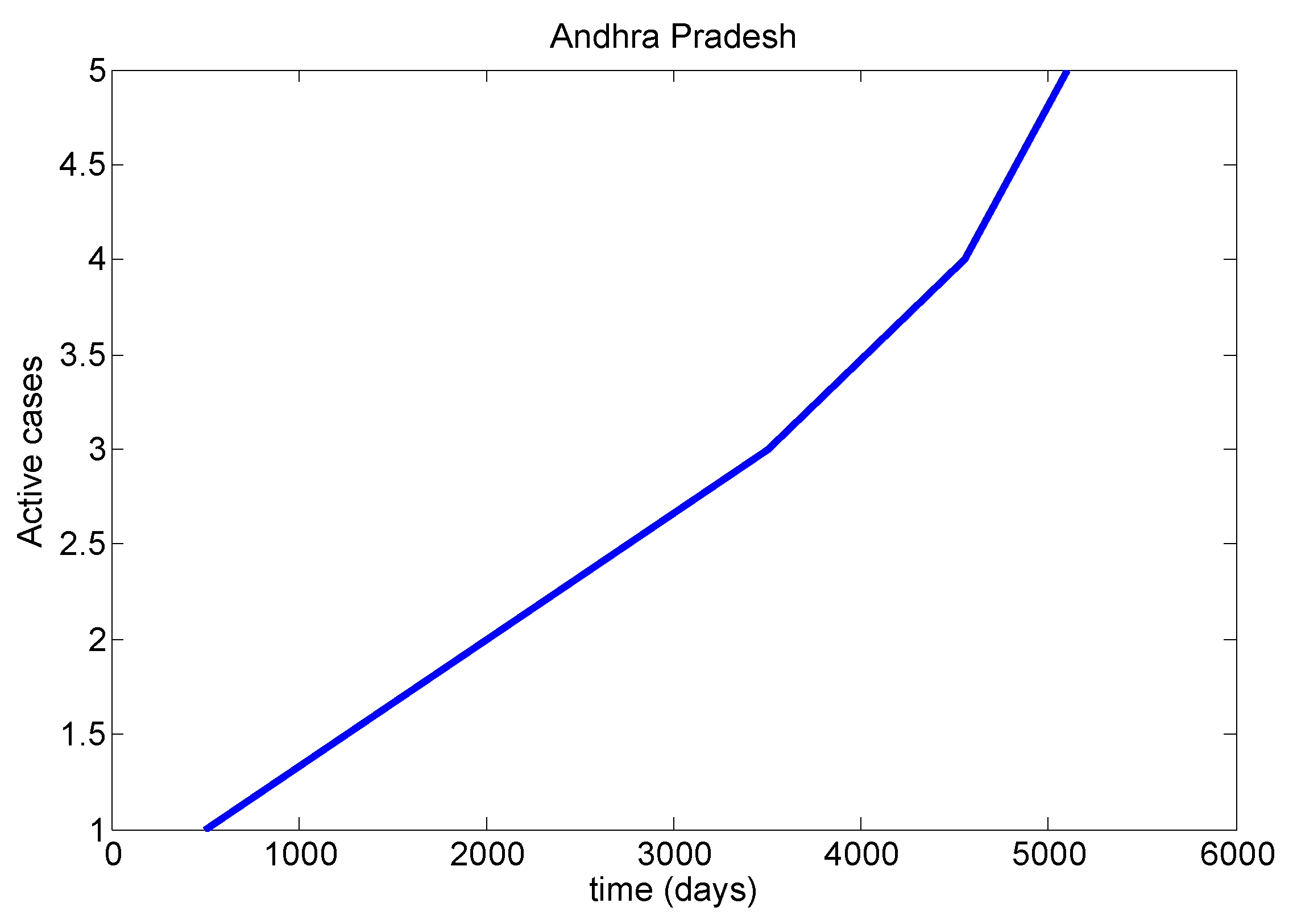
In this section, we discussed five affected states (Maharashtra, Kerala, Karnataka, Tamil Nadu, Andra Pradesh) in India. The four important parameter values (confirmed, active, recovered, deceased) are given in Table 5. Table 6 shows an initial values of the parameters in the states of Maharashtra, Kerala, Karnataka, Tamil Nadu and Andhra Pradesh. We have discussed the Omicron number of cases and initial values (See Table 7 and Table 8). We mainly discussed one parameter for active cases in Maharashtra, Kerala, Karnataka, Tamil Nadu and Andhra Pradesh. We have drawn a diagram for all states at active cases (see Figure 7, Figure 8, Figure 9, Figure 10 and Figure 11). It has given guidelines for international arrivals from January 2022. It is mandatory for self declaration form and RT-PCR test. This approach is given by algorithmic model [45]. If it is negative, home quarantine for one week. If suppose positive, we can send for genomic test and provide isolation facility. It used for proposed model validation from real life data and this case approximately equal to the proposed mathematical model. So this model helps for our future prediction from current data.
We have verified real life data for five highly affected states with other states in India. There are several authors published research articles based on the COVID-19 data details taken from their own countries. It is important to say that still there is no common COVID-19 equation to be utilized in Indian pandemic and to eradicate this disease. Right now, there is no common COVID-19 equation in Indian pandemic. Therefore, we propose a Common Indian COVID-19 Equation which can predict the infection rate and give the control strategies of spread. The aim of the paper is to find out a new model that is common to the Indian COVID-19 pandemic. This model remains the same in India but the parameter values and data will be different based on the present COVID-19 pandemic reports. The required data of COVID-19 will be collected from the WHO (World Health Organization) & Ministry of Health and Family Welfare (MoHFW) up to till date. The nonlinear least square algorithm will be used for getting values to calculate all parameters of the developing model. In our model there is no assumed data. When the data collection and parameter estimation is completed, we have to analyze the stability analysis, analytical solutions, numerical solutions, error analysis and statistical approach. Finally, the statistical approach is compared to real life data to check the validity of the theoretical outcome of new COVID-19 equations. As per the proposed plan, it is assumed that the infection rate of COVID-19 will be decreased very soon, based on government control policy. The proposed model is very useful for the current Indian pandemic to predict the future spread and control strategies with great impact. In the current situation, the infected cases of COVID-19 get changed daily. Our model is valid only for the fixed population. We fix the required time in days. Parameter estimation is done by collecting the data up to date. There are two important cases to find the new parameter values for their own countries. The first case is existence of unique solution of all parameters or important parameters. Another case is the individual’s rate of values in unknown parameters. In particular, COVID-19 equations have lot of parameters in current pandemic situation. Few parameter values are exactly and others may be in approximate solutions. It is very difficult to get the unique solutions for all parameters. Dynamic models have to be developed on related identification property. In this paper, our aim is to find out the common model. We believe that this model works well and will be useful for the Indian people. Based on the data, the model will be changed the susceptible cases, exposed cases, Infective cases, Recovery cases, etc., (SIR, SEIR, SEIRS, etc.). Finally, our model compares to COVID-19 data and validates the outcome system. The proposed model helps the Indian government and other researchers with COVID-19. In the third wave, it sweeps positive surges to 15%. The spread of the third wave is fast and be careful to this current situation.

9. Conclusions

This article plays the dynamics in second wave COVID-19 and newly infected cases for Omicron which have emerged recently in India. The homotopy perturbation method was used to solve the analytical solutions of the dynamics model of second wave COVID-19 with the given initial conditions is effectively analyzed. This method is simple, easy to apply and it provides most approximate analytical expressions. HPM provides an explicit solution which is very useful to analyze the epidemic model based COVID-19 by understanding the parameters. In numerical simulation part, we used Mathematica 12 software for up to 8th order approximation with error analysis which calculated from residual error, absolute error and square error respectively. The growth of the dangerous corona virus and Omicron deadly disease in the current pandemic yields the death of millions of people still date. The basic reproduction number R 0 ranges calculated between 0.8454 and 2.0317 from numerical simulation, derived from analytical approach, it helps to identify the spread of the disease. Finally, our proposed model is verified from the real life data of second wave COVID-19 and Omicron variant, it obtained the validity of the system of equations, the same model is defined to fit all future data. Now Omicron variant is slowly increasing all over world and it is possible to implement lock down for mid of 2022 (June) in India and we conclude that the third wave may be either high spread or less at the end of May 2022.

Author Contributions

Conceptualization, A.M. and B.S.; methodology, A.M. and B.S.; software, K.R.; validation, S.B.; formal analysis, B.S.; investigation, A.M.; resources, V.V.; data curation, V.V.; writing—original draft preparation, B.S; writing—review and editing, A.M. and B.S.; visualization, K.R. and S.B.; supervision, resources, funding acquisition, P.M. and M.H. All authors have read and agreed to the published version of the manuscript.

Funding

The authors would like to thank Taif University Researchers Supporting Project (number TURSP-2020/26), Taif University, Taif, Saudi Arabia.

Data Availability Statement

Indian council of medical research (ICMR), government of India. https://icmr.nic.in (accessed on 14 December 2020). Ministry of health and welfare, government of India. https://www.mohfw.gov.in (accessed on 14 December 2020). National institution for transforming india (NITI Aayog), government of India. https://niti.gov.in (accessed on 14 December 2020). Official updates coronavirus, COVID-19 in India, government of India. https://www.mygov.in/covid-19 (accessed on 14 December 2020).

Conflicts of Interest

The authors declare no conflict of interest.

References

  1. Poongodi, M.; Al-Shaikhli, I.F.; Vijayakumar, V. The Probabilistic Approach of Energy Utility and Reusability Model with Enhanced Security from the Compromised Nodes through Wireless Energy Transfer in WSN. Int. J. Pure Appl. Math. 2017, 116, 233–250. [Google Scholar]
  2. Jeyachandran, A.; Poongodi, M. Securing Cloud information with the use of Bastion Algorithm to enhance Confidentiality and Protection. Int. J. Pure Appl. Math. 2018, 118, 1–13. [Google Scholar]
  3. Poongodi, M.; Vijayakumar, V.; Ramanathan, L.; Gao, X.Z.; Bhardwaj, V.; Agarwal, T. Chat-bot-based natural language interface for blogs and information networks. Int. J. Web Based Communities 2019, 15, 178–195. [Google Scholar]
  4. Poongodi, M.; Vijayakumar, V.; Chilamkurti, N. Bitcoin price prediction using ARIMA model. Int. J. Internet Technol. Secur. Trans. 2020, 10, 396–406. [Google Scholar] [CrossRef]
  5. Poongodi, M.; Hamdi, M.; Varadarajan, V.; Rawal, B.S.; Maode, M. Building an Authentic and Ethical Keyword Search by applying Decentralised (Blockchain) Verification. In Proceedings of the IEEE INFOCOM 2020—IEEE Conference on Computer Communications Workshops (INFOCOM WKSHPS), Toronto, ON, Canada, 6–9 July 2020; pp. 746–753. [Google Scholar]
  6. Poongodi, M.; Bose, S. The COLLID based intrusion detection system for detection against DDOS attacks using trust evaluation. Adv. Nat. Appl. Sci. 2015, 9, 574–580. [Google Scholar]
  7. Poongodi, M.; Bose, S. Stochastic model: ReCAPTCHA controller based co-variance matrix analysis on frequency distribution using trust evaluation and re-eval by Aumann agreement theorem against DDoS attack in MANET. Clust. Comput. 2015, 18, 1549–1559. [Google Scholar] [CrossRef]
  8. Chakraborty, T.; Ghosh, I. Real-time forecasts and risk assessment of novel coronavirus (COVID-19) cases: A data-driven analysis. Chaos Solitons Fractals 2020, 135, 109850. [Google Scholar] [CrossRef]
  9. Fanelli, D.; Piazza, F. Analysis and forecast of COVID-19 spreading in China, Italy and France. Chaos Solitons Fractals 2020, 134, 109761. [Google Scholar] [CrossRef]
  10. Hellewell, J.; Abbott, S.; Gimma, A.; Bosse, N.I.; Jarvis, C.I.; Russell, T.W.; Munday, J.D.; Kucharski, A.J.; Edmunds, W.J.; Sun, F.; et al. Feasibility of controlling COVID-19 outbreaks by isolation of cases and contacts. Lancet Glob. Health 2020, 8, e488–e496. [Google Scholar] [CrossRef] [Green Version]
  11. Indian Council of Medical Research (ICMR), Government of India. 2020. Available online: https://icmr.nic.in (accessed on 14 December 2020).
  12. Kar, T.; Nandi, S.K.; Jana, S.; Mandal, M. Stability and bifurcation analysis of an epidemic model with the effect of media. Chaos Solitons Fractals 2019, 120, 188–199. [Google Scholar] [CrossRef]
  13. Kucharski, A.J.; Russell, T.W.; Diamond, C.; Liu, Y.; Edmunds, J.; Funk, S.; Eggo, R.M.; Sun, F.; Jit, M.; Munday, J.D.; et al. Early dynamics of transmission and control of COVID-19: A mathematical modelling study. Lancet Infect. Dis. 2020, 20, 553–558. [Google Scholar] [CrossRef] [Green Version]
  14. Liu, Y.; Gayle, A.A.; Wilder-Smith, A.; Rocklöv, J. The reproductive number of COVID-19 is higher compared to SARS coronavirus. J. Travel Med. 2020, 5, 1–4. [Google Scholar] [CrossRef] [PubMed] [Green Version]
  15. Mizumoto, K.; Chowell, G. Transmission potential of the novel coronavirus (COVID-19) onboard the diamond Princess Cruises Ship, 2020. Infect. Dis. Model. 2020, 5, 264–270. [Google Scholar] [CrossRef] [PubMed]
  16. Ndaïrou, F.; Area, I.; Nieto, J.J.; Torres, D.F. Mathematical modeling of COVID-19 transmission dynamics with a case study of Wuhan. Chaos Solitons Fractals 2020, 135, 109846. [Google Scholar] [CrossRef]
  17. Prem, K.; Liu, Y.; Russell, T.W.; Kucharski, A.J.; Eggo, R.M.; Davies, N.; Flasche, S.; Clifford, S.; Pearson, C.A.; Munday, J.D.; et al. The effect of control strategies to reduce social mixing on outcomes of the COVID-19 epidemic in Wuhan, China: A modelling study. Lancet Public Health 2020, 5, e261–e270. [Google Scholar] [CrossRef] [Green Version]
  18. Ribeiro, M.H.D.M.; da Silva, R.G.; Mariani, V.C.; dos Santos Coelho, L. Short-term forecasting COVID-19 cumulative confirmed cases: Perspectives for Brazil. Chaos Solitons Fractals 2020, 135, 109853. [Google Scholar] [CrossRef]
  19. Adamu, H.A.; Muhammad, M.; Jingi, A.; Usman, M. Mathematical modelling using improved SIR model with more realistic assumptions. Int. J. Eng. Appl. Sci. 2019, 6, 64–69. [Google Scholar] [CrossRef]
  20. Rajendrakumar, A.L.; Nair, A.T.N.; Nangia, C.; Chourasia, P.K.; Chourasia, M.K.; Syed, M.G.; Nair, A.S.; Nair, A.B.; Koya, M.S.F. Epidemic landscape and forecasting of SARS-CoV-2 in India. J. Epidemiol. Glob. Health 2021, 11, 55–59. [Google Scholar] [CrossRef]
  21. Crowdsourced India COVID-19 Tracker Data. Available online: https://bit.ly/patientdb (accessed on 14 December 2020).
  22. Lopez, L.; Roda, X. A Modified SEIR Model to Predict COVID-19 Outbreak in Spain and Italy: Simulating Control Scenarios and Multi Scale Epidemics. 2020. Available online: https://www.medrxiv.org/content/10.1101/2020.03.27.20045 (accessed on 14 December 2020).
  23. Ministry of Health and Family Welfare, Government of India. District Wise List of Reported Cases Our World in Data: Coronavirus Source Data. 2020. Available online: https://ourworldindata.org/coronavirus-source-data (accessed on 14 December 2020).
  24. Peng, L.; Yang, W.; Zhang, D.; Zhuge, C.; Hong, L. Epidemic Analysis of COVID-19 in China by Dynamic Modelling. 2020. Available online: https://www.medrxiv.org/content/10.1101/2020.02.16.20023 (accessed on 14 December 2020).
  25. Sanders, J.M.; Monogue, M.L.; Jodlowski, T.Z.; Cutrell, J.B. Pharmacologic treatments for coronavirus disease 2019 (COVID-19): A review. JAMA 2020, 323, 1824–1836. [Google Scholar] [CrossRef] [PubMed]
  26. Khan, M.A.; Atangana, A. Modeling the dynamics of novel coronavirus (2019-nCoV) with fractional derivative. Alex. Eng. J. 2020, 59, 2379–2389. [Google Scholar] [CrossRef]
  27. Bai, Y.; Yao, L.; Wei, T.; Tian, F.; Jin, D.-Y.; Chen, L.; Wang, M. Presumed asymptomatic carrier transmission of COVID-19. JAMA 2020, 323, 1406–1407. [Google Scholar] [CrossRef] [PubMed] [Green Version]
  28. Bekiryazici, Z.; Merdan, M.; Kesemen, T. Modification of the random differential transformation method and its applications to compartmental models. Commun.-Stat.-Theory Methods 2020, 6, 1–22. [Google Scholar] [CrossRef]
  29. Chen, T.-M.; Rui, J.; Wang, Q.-P.; Zhao, Z.-Y.; Cui, J.-A.; Yin, L. A mathematical model for simulating the phase-based transmissibility of a novel coronavirus. Infect. Dis. Poverty 2020, 9, 1–8. [Google Scholar] [CrossRef] [Green Version]
  30. Choi, S.; Ki, M. Estimating the reproductive number and the outbreak size of COVID-19 in Korea. Epidemiol. Health 2020, 42, e2020011. [Google Scholar] [CrossRef] [PubMed]
  31. Danane, J.; Allali, K.; Hammouch, Z. Mathematical analysis of a fractional differential model of HBV infection with antibody immune response. Chaos Solitons Fractals 2020, 136, 109787. [Google Scholar] [CrossRef]
  32. Hamada, Y.M. Solution of a new model of fractional telegraph point reactor kinetics using differential transformation method. Appl. Math. Model. 2020, 78, 297–321. [Google Scholar] [CrossRef]
  33. Lin, Q.; Zhao, S.; Gao, D.; Lou, Y.; Yang, S.; Musa, S.S.; Wang, M.H.; Cai, Y.; Wang, W.; Yang, L.; et al. A conceptual model for the coronavirus disease 2019 (COVID-19) outbreak in Wuhan, China with individual reaction and governmental action. Int. J. Infect. Dis. 2020, 93, 211–216. [Google Scholar] [CrossRef]
  34. Roda, W.C.; Varughese, M.B.; Han, D.; Li, M.Y. Why is it difficult to accurately predict the COVID-19 epidemic? Infect. Dis. Model. 2020, 5, 271–281. [Google Scholar] [CrossRef]
  35. Shaikh, A.S.; Shaikh, I.N.; Nisar, K.S. A mathematical model of COVID-19 using fractional derivative: Outbreak in India with dynamics of transmission and control. Adv. Differ. Equ. 2020, 2020, 1–19. [Google Scholar] [CrossRef]
  36. Veeresha, P.; Prakasha, D.G.; Malagi, N.S.; Baskonus, H.M.; Gao, W. New dynamical behaviour of the Corona-virus (COVID-19) infection system with nonlocal operator from reservoirs to people. Res. Sq. 2020, 5, 1–18. [Google Scholar]
  37. World Health Organization. Coronavirus Disease 2019. Available online: https://www.who.int/health-topics/Corona-virus (accessed on 14 December 2020).
  38. Kirk, D.E. Optimal Control Theory: An Introduction; Dover Publications: New York, NY, USA, 2012. [Google Scholar]
  39. Lenhart, S.M.; Workman, J.T. Optimal Control Applied to Biological Models; CRC Press: Boca Raton, FL, USA, 2007; Volume 15. [Google Scholar]
  40. Wang, X. Solving Optimal Control Problems with MATLAB: Indirect Methods; ISE Dept., NCSU: Raleigh, NC, USA, 2009. [Google Scholar]
  41. Available online: https://arogya.maharashtra.gov.in/1177/Dedicated-COVID-Facilities-Status (accessed on 14 December 2020).
  42. Available online: https://stopcorona.tn.gov.in/ (accessed on 14 December 2020).
  43. Available online: https://karunadu.karnataka.gov.in/hfw/nhm/pages/home.aspx (accessed on 14 December 2020).
  44. Available online: http://hmfw.ap.gov.in/COVID-19%20IEC/COVID-19%20Hospitals.pdf (accessed on 14 December 2020).
  45. Available online: https://www.mea.gov.in/guidelines-for-international-arrivals.htm (accessed on 14 December 2020).
Figure 1. The compartmental diagram for COVID-19 epidemic model.
Mathematics 10 00343 g001
Figure 2. The residual error of 8th order approximation for E R 1 , E R 2 , E R 3 , E R 4 , E R 5 and E R 6 .
Mathematics 10 00343 g002
Figure 3. The Absolute error of 8th order approximation for E R 1 , E R 2 , E R 3 , E R 4 , E R 5 and E R 6 .
Mathematics 10 00343 g003
Figure 4. The h curves initial derivatives of 7th and 8th order approximation from HPM.
Mathematics 10 00343 g004
Figure 5. The Square residual error of 8th order approximation.
Mathematics 10 00343 g005
Figure 6. The basic reproduction number calculated from number of cases on real life data, (a) number of cases 80% increased, (b) number of cases 20% increased, (b) number of cases 10% increased, (d) number of cases 60% increased, (e) number of cases 40% increased, (f) number of cases 20% increased, (g) number of cases 60% increased, (h) number of cases 5% increased.
Mathematics 10 00343 g006
Figure 7. Active cases of Maharshtra from real life data.
Mathematics 10 00343 g007
Figure 8. Active cases of Kerala from real life data.
Mathematics 10 00343 g008
Figure 9. Active cases of Karnataka from real life data.
Mathematics 10 00343 g009
Figure 10. Active cases of Tamil Nadu from real life data.
Mathematics 10 00343 g010
Figure 11. Active cases of Andhra Pradesh from real life data.
Mathematics 10 00343 g011
Table 1. The proposed model variables and parameters description.
S ( t ) Susceptible people
E ( t ) Exposed people
I ( t ) Infected strength
I a ( t ) Asymptotically infected people
R ( t ) Recovered people
M ( t ) Reservoir people
α 0 Birth rates
α 1 death rates
α 2 Coefficient of transmission
α 3 Multiple transmission
α 4 Disease transmission
α 5 Infection of Asymptomatic
α 6 Incubation parameter
α 7 Infected transmission
α 8 Rate of recovery
α 9 Asymptomatic peoples
α 10 Virus transmission of Asymptomatic
α 11 Virus transmission of reservoir
Table 2. The h values range of Compartments.
S ( t ) −1.1 ≤ h ≤ −0.4
E ( t ) −1.3 ≤ h ≤ −0.8
I ( t ) −1.4 ≤ h ≤ −0.7
I a ( t ) −1.5 ≤ h ≤ −0.4
R ( t ) −1.7 ≤ h ≤ −0.2
M ( t ) −1.8 ≤ h ≤ −0.1
Table 3. The optimal solutions of S h 1 * , E h 2 * ,   I h 3 * ,   I a h 4 * ,   R h 5 * ,   M h 6 * .
h*Optimum Solution of Compartment
S ( h 1 ) −1.12 × 10 4
E ( h 2 ) −1.23 × 10 6
I ( h 3 ) −1.34 × 10 8
I a ( h 4 ) −1.45 × 10 10
R ( h 5 ) −1.56 × 10 12
M ( h 6 ) −1.67 × 10 14
Table 4. The residual errors for E R 1 ,   E R 2 ,   E R 3   E R 4 ,   E R 5 and E R 6 for t 0 , 1 .
tER 1 ER 2 ER 3 ER 4 ER 5 ER 6
0.03.4 × 10 1 2.3 × 10 1 1.1 × 10 1 1.8 × 10 1 3.1 × 10 1 1.9 × 10 1
0.11.2 × 10 2 4.7 × 10 2 6.8 × 10 2 2.5 × 10 2 4.5 × 10 2 3.6 × 10 2
0.24.5 × 10 3 9.9 × 10 3 4.2 × 10 3 9.2 × 10 3 9.2 × 10 3 4.9 × 10 3
0.31.1 × 10 4 6.7 × 10 4 3.3 × 10 4 8.3 × 10 4 6.3 × 10 4 9.2 × 10 4
0.46.1 × 10 5 3.5 × 10 5 2.1 × 10 5 7.5 × 10 5 5.5 × 10 5 8.7 × 10 5
0.57.3 × 10 6 1.9 × 10 6 5.9 × 10 6 1.6 × 10 6 4.9 × 10 6 5.4 × 10 6
0.65.6 × 10 7 2.7 × 10 7 6.3 × 10 7 1.5 × 10 7 3.7 × 10 7 9.1 × 10 7
0.72.8 × 10 8 4.4 × 10 8 7.5 × 10 8 3.8 × 10 8 2.9 × 10 8 2.6 × 10 8
0.83.7 × 10 9 6.1 × 10 9 2.2 × 10 9 4.9 × 10 9 1.6 × 10 9 3.9 × 10 9
0.94.9 × 10 10 7.8 × 10 10 3.9 × 10 10 5.6 × 10 10 2.9 × 10 10 4.1 × 10 10
15.1 × 10 11 9.1 × 10 11 4.9 × 10 11 9.2 × 10 11 8.4 × 10 11 8.8 × 10 11
Table 5. Number of COVID-19 cases across Indian states and union territories as of 25 October 2021.
ParametersMaharashtraKeralaKarnatakaTamil NaduAndra PradeshReferences
confirmed6,602,9614,915,3312,985,9862,695,2162,063,577[41,42,43,44]
Active27,50677,964874013,0345102[41,42,43,44]
Recovered6,435,4394,808,7752,939,2392,646,1632,044,132[41,42,43,44]
Deceased140,01628,59238,00736,01914,343[41,42,43,44]
Table 6. Initial Values of parameters in the states of Maharashtra, Kerala, Karnataka, Tamil Nadu and Andhra Pradesh.
Initial ValuesMaharashtraKeralaKarnatakaTamil NaduAndra PradeshReferences
S(0)3,301,4802,515,3001,590,9001,390,3001,070,600[41,42,43,44]
E(0)13,50035,8004700680,1505,060,300Calculated
I(0)70,01617,599280060405000[41,42,43,44]
Ia(0)35009000140032002500[41,42,43,44]
R(0)3,234,4002,408,7001,540,3001,340,1701,040,100[41,42,43,44]
M(0)1,630,50014,60019,008730,1697400Calculated
Table 7. Number of Omicron cases across Indian states and union territories as of 30 December 2021.
ParametersMaharashtraKeralaDelhiGujaratRajasthanReferences
confirmed141571424943[41,42,43,44]
Active90401103032[41,42,43,44]
Recovered50301598[41,42,43,44]
Deceased12242[41,42,43,44]
Table 8. Initial Values of parameters in the states of Maharashtra, Kerala, Delhi, Gujarat and Rajasthan.
Initial ValuesMaharashtraKeralaDelhiGujaratRajasthanReferences
S(0)0.50.50.50.50.5[41,42,43,44]
E(0)0.30.20.10.30.2[41,42,43,44]
I(0)0.10.10.10.20.2[41,42,43,44]
Ia(0)0.10.20.10.20.1[41,42,43,44]
R(0)0.20.20.20.10.1[41,42,43,44]
M(0)0.20.10.10.20.2[41,42,43,44]
Publisher’s Note: MDPI stays neutral with regard to jurisdictional claims in published maps and institutional affiliations.

