Spreading of Infections on Network Models: Percolation Clusters and Random Trees

Abstract

We discuss network models as a general and suitable framework for describing the spreading of an infectious disease within a population. We discuss two types of finite random structures as building blocks of the network, one based on percolation concepts and the second one on random tree structures. We study, as is done for the SIR model, the time evolution of the number of susceptible (S), infected (I) and recovered (R) individuals, in the presence of a spreading infectious disease, by incorporating a healing mechanism for infecteds. In addition, we discuss in detail the implementation of lockdowns and how to simulate them. For percolation clusters, we present numerical results based on site percolation on a square lattice, while for random trees we derive new analytical results, which are illustrated in detail with a few examples. It is argued that such hierarchical networks can complement the well-known SIR model in most circumstances. We illustrate these ideas by revisiting USA COVID-19 data.

1. Introduction

The interest in understanding and modeling epidemics spreading in humans has surged conspicuously since the outbreak of the COVID-19 phenomenon (see e.g., [1,2,3,4,5,6,7,8,9]). It is generally accepted that the mathematical framework for epidemics relies on the seminal work by Kermack and McKendrick (1927) who introduced the SIR model [10], now regarded as the ‘benchmark’ for describing the time evolution of infectious diseases over a wealth of different situations. For reviews see e.g., the classical work by Hethcote [11], including several analytical results, and also a more recent compendium [12]. Spreading phenomena has a long history both on the mathematical aspects (see e.g., [13]), as well as on the modeling of epidemics outbreak and control of their evolution [14,15,16]. It has been studied extensively also in the realm of statistical physics of disordered systems (e.g., [17,18,19]). More recently, a great deal of interest has been devoted to the study and development of new scenarios to describe COVID-19 spreading [20,21,22,23,24,25,26,27,28,29,30,31,32,33,34,35]. In addition, we can mention that a lot of attention has been drawn to population structures displaying complex and heterogeneous connectivity patterns, as well as to the associated dynamics of epidemic and infection spreading processes in the so-called metapopulation models [36,37].

Recently, a network model based on lattice site percolation concepts has been introduced to describe the spreading of a virus within a population aimed at complementing the widely used SIR model, especially within the context of COVID-19 outbreak [9]. In the model, the sites of a square lattice are occupied with probability p and are defined as susceptibles (individuals who can become infected by the infectious disease), while the remaining unoccupied sites are considered to be inactive or immune individuals, denoted as dormants. In the case $p=1$, the whole lattice represents a simple connectivity graph among a fixed number N of individuals within a population, where $N=L^2$ and L is the linear size of the square lattice. An example of the percolation model, before the breakout of the disease, in the case of interest here, i.e., $p=1/2$, is illustrated in Figure 1. The latter must be understood as a ‘correlation matrix’, or probability of contact between individuals, rather than actual locations in coordinate space.

Essentially, the network model represents an extension of the widely used SIR model, valid for a spatially uniform distribution of individuals in different categories, to the more realistic situation in which they are organized in clusters of individuals with strong connectivity correlations. In a sense, the network model can be also seen as a type of generalized ‘mean-field’ approach in which a spreading dynamics is solved ‘exactly’ within each cluster, followed by an average over different clusters.

In this work, we generalize the percolation model studied in [9], based on the idea that infection spreading can occur among appropriately defined clusters, representing otherwise well isolated communities, which become interconnected dynamically as infection spreads within the network. The clusters are constructed or designed in such a way that their internal spreading dynamics can be solved ‘exactly’, either numerically or analytically, and their contributions to the total infections in the network can be added sequentially say, such that one can mimic the time evolution of the infectious disease in a real situation. We discuss how the number of clusters participating in the network can be adjusted to reproduce the speeding up of the number of infecteds at the initial stages of the breakout, and how lockdowns can be simulated in a simple fashion. We discuss two different approaches to this problem which can be used for describing real spreading data. The method allows in a very simple and rapid way to create and study different possible scenarios once the internal cluster spreading dynamics has been solved. This approach has thus the advantage of requiring limited computational resources.

The paper is organized as follows. In Section 2, we define the network model, first in terms of a generic hierarchical structure, both in the transmission times as well as in the internal structure of the constituent clusters to motivate the present approach, followed by a detail discussion of the specific modeling used here. In Section 3, we deal with a specific type of clusters, which we call minor clusters, represented by finite percolation clusters of the type considered in [9]. We solve the spreading dynamics on these minor clusters in Section 3.1, in order to introduce the SIR categories in the problem and discuss how to implement the healing times for infected individuals. Then, in Section 3.2 we show how to create a network from the minor clusters and discuss the implementation of lockdowns in the network. In Section 4, we discuss an exactly solvable model for minor clusters based on random trees. We consider first the effects of healing in Section 4.1, followed by a treatment of lockdowns without healings in Section 4.2. The combination of both healings and lockdowns in a tree is discussed in Section 4.3. These results, although interesting in their own right, can be used also as building blocks of a more general network of random trees. In Section 5, we apply the random trees results to the analysis of USA COVID-19 data. Technical details are relegated to an Appendix A. Finally, in Section 6 we present our conclusions.

2. Network Model: A Hierarchical Structure of Transmission Times

Let us discuss the assumptions behind the present network model. The basic idea is that the population is organized in well separated (disjoint) clusters, each one constituted by well connected (susceptible) individuals. This is more a working hypothesis than a proved statement. However, keeping this in mind, we may argue that it may well reflect reality, at least within a finite period of time, eventually shorter than the time scale of the disease outbreak. In order to substantiate the concept, we need to determine the network structure, which is schematically illustrated in Figure 2. In general, each ‘major cluster’ (such as those indicated in blue color in the figure), maybe built upon several minor (white) clusters (say, 3 in the case of cluster 1; 2 in cluster 2, etc.). The difference between clusters resides in the different time scales, ${\tau }_{x,y}$, for infection transmission. Within minor clusters, the person-to-person contact frequency is the highest (${\tau }_{a,a}$ is the shortest); between minor clusters the frequency is lower (${\tau }_{a,b}>{\tau }_{a,a}\cong {\tau }_{b,b}$); while between major clusters (say between 1 and 2) the contact frequency is the lowest (i.e., ${\tau }_{1,2}\gg {\tau }_{a,b}$). This may correspond to a kind of hierarchical distribution of transmission times, which is determined by the connectivity structure of the network.

In Figure 2, the red arrows depict a possible path for infection spreading. We would like to note that this transmission path is not determined a priori, but it occurs at random as the process evolves in time. Note also the possibility of a direct transmission between minor clusters belonging to different major clusters, such as for instance the red line connecting minor cluster b (from major cluster 2) to minor cluster c (within major cluster 3). These links will play a crucial role in our work here. We also note that the effect of lockdowns can be implemented by assuming much larger inter-major-cluster transmission times (for example, ${\tau }_{3,6}\gg {\tau }_{3,4}$), or by completely hindering transmission between major clusters, so that infection can go on only inside already infected clusters. In addition to these transmission time scales, there are a few more features to consider, i.e., incubation and latent periods, and healing and contagious periods. If the latent period is shorter than the incubation one, infectiousness can propagate undetected for a while. If incubation time is much shorter than latency, then symptoms manifest before infectiousness occurs. We will not discuss the former cases in this work, but they can be implemented in specific applications. Rather, more important to us are the latter, that is the possibility of healing (or end of the contagious condition) after a time say, ${\tau }_{\mathrm{H}}>{\tau }_{i,j}$, where $(i,j)$ are major cluster indices.

The implementation of a realistic distribution of clusters requires a thoroughly analysis of the population structure, accompanied by a sophisticated acquisition of real data. It is interesting to note that the concept highlighted in Figure 2 has implicitly been applied to the problem of tracing actual trajectories followed by infected individuals (see e.g., [38,39]). Thus, the idea of a hierarchy of transmission times is of course not new. However, for the clarity of presentation, and to avoid any misunderstanding, it is convenient to delineate the strategy of our work for dealing with the construction of a network.

To this end, let us formally write the total number of infected individuals, $I\left(t\right)$, at time t in a population network in general as,

$$I\left(t\right)=\sum _{i=1}^{N_c}{I}_i(t-t_i)\Theta (t-t_i),$$

(1)

where $I_i(t-t_i)$ represents the number of infecteds within the ith cluster, $t_i$ the time at which the first individual from cluster i becomes infected, and $N_c$ is the total number of clusters considered. The $\Theta$-function, defined as $\Theta \left(x\right)=1$ for $x\ge 1$ and $\Theta \left(x\right)=0$ otherwise, ensures that only infected clusters contribute to $I\left(t\right)$. The distribution of transmission times, ${\tau }_{i,j}$, between clusters i and j is encoded in the activation times $t_i$, in the sense that cluster i becomes ‘activated’ by an infected from a previously infected cluster j. It is important to realize that the transmission process is dynamical in nature, when an infected from cluster j meets one susceptible from cluster i. This will be denoted as a non-local transmission (for instance the minor-minor $b\to c$ transmission in Figure 2), as opposed to a local one taking place inside a single minor cluster. The place where this happens can be anywhere, and the newly infected individual can spread the virus within the community of origin (the ith minor cluster) once back there. One can expect these non-local transmissions to occur at random and being hard to trace or predict due to the complexity of the system [38,39].

To proceed further, we then concentrate on the dynamics of spreading, $I_i\left(t\right)$, on minor clusters only, while the intrinsically time-dependent behavior of non-local transmissions is taken implicitly into account through a suitable choice of the activation times $t_i$, the latter estimated from the empirical data as we discuss below. This model does not rely on any specific structure of a population, and its aim is to describe the temporal evolution of infection in an average sense. The advantages of this approach over standard SIR calculations are: The possibility of fitting huge empirical data very efficiently using exact analytical expressions, providing an alternative information on the effective infection rate in a population as a function of time, and open up the possibility of estimating the effective size distribution of communities involved in the infection spreading phenomenon.

As models for minor clusters, we study finite percolation clusters in two dimensions below the percolation transition, and random expanding trees. Although $I_i\left(t\right)$ for percolation clusters can be solved only numerically, random trees admit simple analytical solutions, making them more attractive for describing spreading phenomena in complex situations. We review percolation clusters first, also for the purpose of discussing our previous percolation model [9] from a more general perspective.

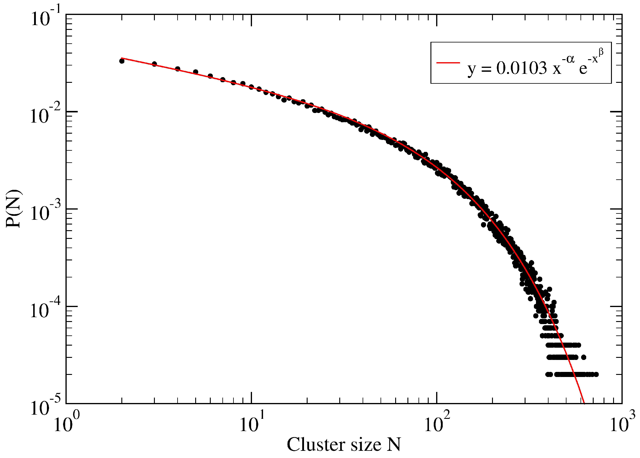
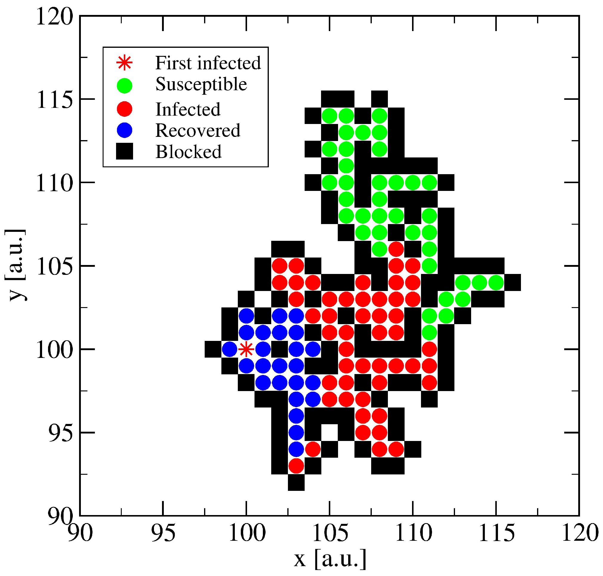
3. A Percolation Model for Minor Clusters: Cluster Sizes

The minor clusters referred to in Figure 2 constitute the smallest social structures considered in the model. They are at the core of the dynamical behavior of spreading, and therefore require a detailed and specific description. Eventually, the dynamical ‘solution’ of a ‘typical’ minor cluster can be used to describe, in a first approximation, the behavior of the network on longer time scales, as we will discuss below. To this end, we follow the network approach discussed in [9], and represent our core structures as finite percolation clusters, below the nearest-neighbor (NN) site percolation threshold, on the square lattice, $p_c\cong 0.593$ (Figure 3).

The dimensionality two, as well as the choice of just NN connectivity, is done for convenience of visual representation and simplicity. Of course, other models can be used if required in particular cases. Now, let us look at how the cluster sizes are distributed in our case. The results are shown in Figure 4 for a sample of ${10}^5$ clusters.

As one can see from Figure 4, finite cluster sizes can be quite large for $p=1/2$, with $N\lesssim 1000$. However, the mean cluster linear extension, $L_N$, scales with cluster size only as $L_N\sim N^{1/d_{\mathrm{f}}}$, where $d_{\mathrm{f}}=91/48\cong 1.895$ is the fractal dimension of percolation clusters in two dimensions [18,19], yielding say, $L\approx 29$ for $N=600$. We have found that a lattice of size (200 × 200) was enough to avoid finite size effects for the sample of ${10}^5$ cluster configurations. In three dimensions, $p_c\cong 0.3116$ and $d_{\mathrm{f}}\cong 2.523$, and spreading becomes even slower [41].

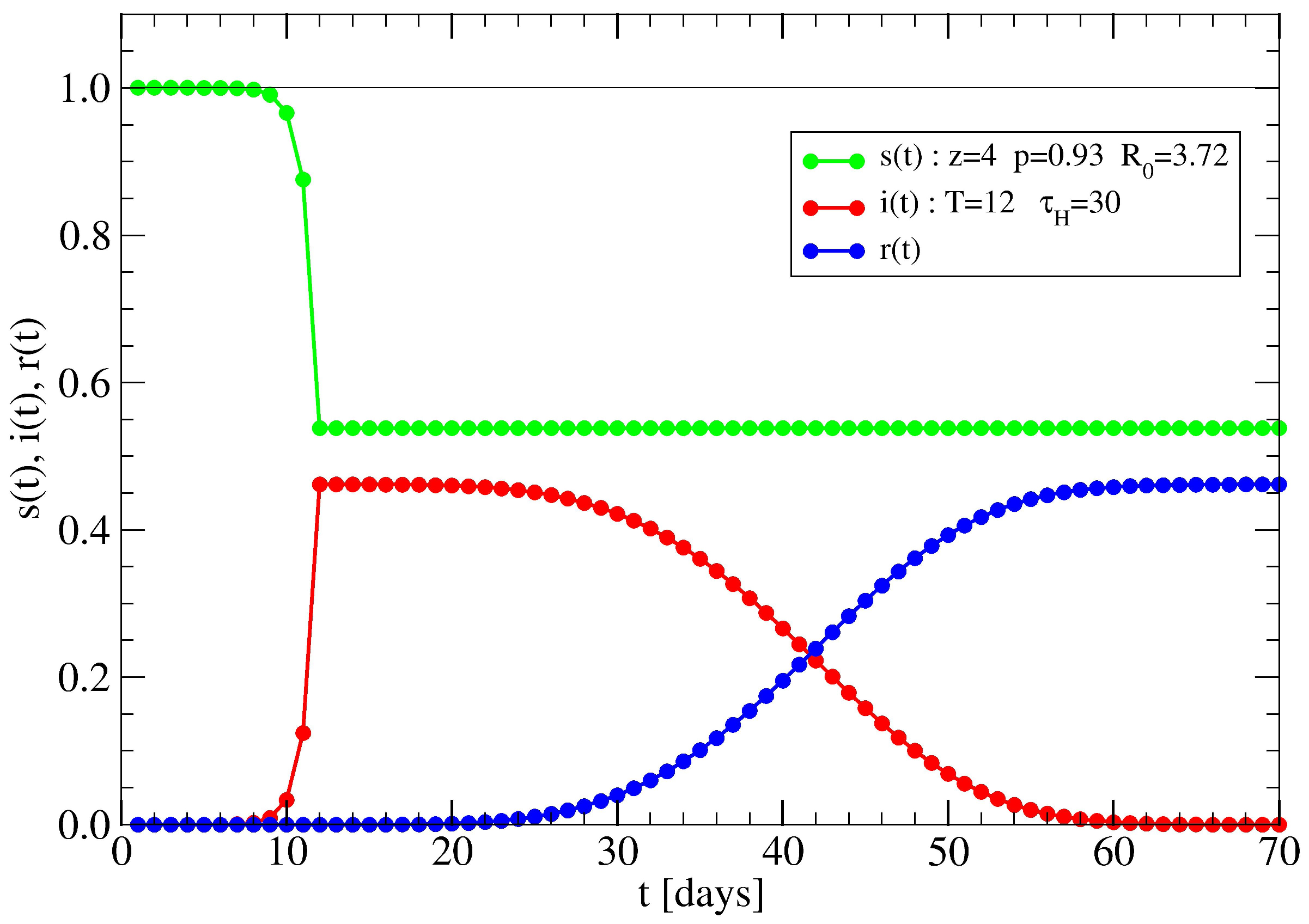
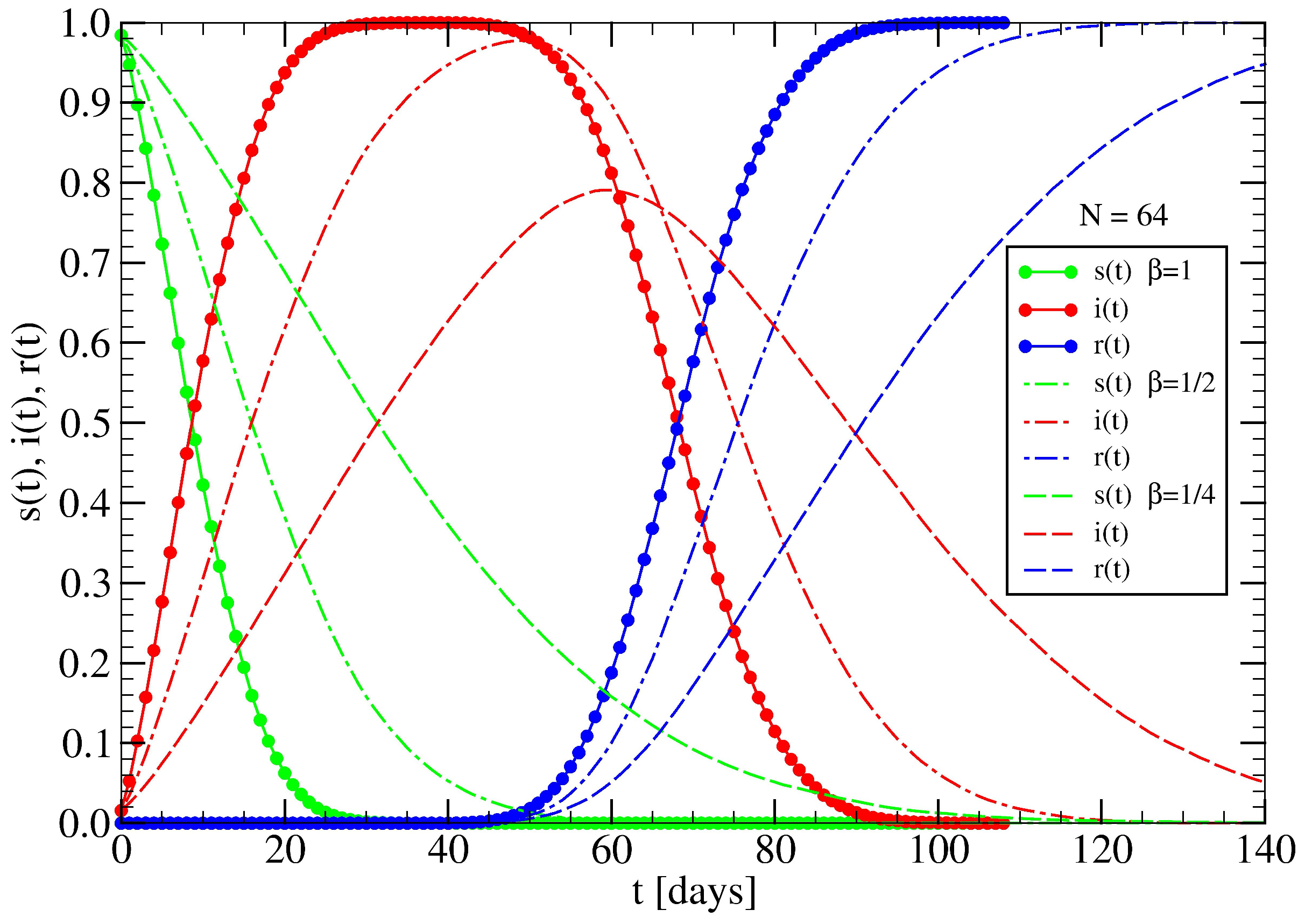
3.1. The Spreading Dynamics on a Minor Cluster

The rules for infection spreading on a minor cluster, modeled by a finite percolation cluster, are very simple. Initially, all available sites in the cluster are taken as susceptibles, while the blocked ones surrounding the cluster cannot be infected. The infection starts (for convenience) at the first created site of the cluster, $k=1$, and it is modeled as a discrete time process of unit time $t_0$ (say $t_0=1$ day); the process starts at time step $t=1$. Then, at time step $t=2$, each one of the available NN sites of k can be infected with a probability $\beta =t_0/{\tau }_{\beta }$, where ${\tau }_{\beta }$ is the time taken for the disease to be transmitted among NN sites, corresponding to the time scale ${\tau }_{a,a}$ in Figure 2. In the case ${\tau }_{\beta }=t_0$ then all available NN sites of k become infected. The infection proceeds from each one of the newly infected sites. We use the terms ‘Infecteds’ and ‘Recovereds’ as abbreviations of ‘Infected individuals’ and ‘Recovered individuals’ (see Figure 5).

Each susceptible site carries a clock which starts ticking when it becomes infected, at say time $t_k$, thus becoming the kth infected site to which we associate the healing time ${\tau }_h\left(k\right)$, taken from the distribution function described in Figure 6. The clock stops ticking at time $t=t_k+{\tau }_h\left(k\right)$ when the site gets healed, becoming a blue site (see e.g., Figure 5).

We illustrate the dynamical behavior of spreading on clusters of size $N=64$, i.e., the mean cluster size in our problem, by averaging the functions $S\left(t\right)$, $I\left(t\right)$ and $R\left(t\right)$ over ${10}^3$ configurations. The results are shown in Figure 7 for the cases $\beta =(1,1/2,1/4)$, corresponding to times ${\tau }_{\beta }=(1,2,4)t_0$. Clearly, all N sites become infected when ${\tau }_{\beta }=t_0$ and, in addition, all susceptibles can be found to be infected simultaneously at some time. This happens when the shortest path, or minimum number of steps connecting any two cluster sites (the so-called ‘topological’ or ‘chemical’ distance [17]), of the farthest site to the first infected site is smaller than the actual minimum healing time in the cluster. In other words, spreading reaches the last susceptible before any of the infecteds are healed.

For larger transmission times ${\tau }_{\beta }$, the process not only slows down but also some susceptibles can remain uninfected. In particular, this can happen if ${\tau }_{\beta }\gtrsim {\tau }_{\mathrm{H}}$. To be noted is that for some clusters, there occurs a sort of ‘bottle neck’, i.e., when different parts of the cluster are connected by a single link. In those cases, spreading becomes so slow (for large enough ${\tau }_{\beta }$) that infection stops spreading due to healings. As we can see, one can describe multiple scenarios with this simple percolation model. For instance, one can argue that a recovered site can still ‘transmit’ the infection, as those individuals with antibodies who may still be able to carry and spread the virus. Such scenarios can be implemented by adding further parameters to the model, but their study goes beyond the scope of the present work.

Each newly infected has, on average, $\kappa =pz$ neighboring susceptibles to infect, where p is the probability that a neighbor is a susceptible (i.e., it is occupied in the language of percolation). For the present infection model, $z=3$ since the coordination number of the square lattice is 4 and, except for the first infected, the newly infecteds can infect at most three neighboring susceptibles. We refer to z with the special name of infection degree. From a given infected then, the infection can be transmitted with a probability $\beta =t_0/{\tau }_{\beta }$ to one susceptible, which remains infectious during the following ${\tau }_h/t_0$ time steps; then it heals. Thus, the mean number of new infecteds from a single infected is $R_0=\kappa min(\beta {\tau }_{\mathrm{H}}/t_0,1)=pzmin({\tau }_{\mathrm{H}}/{\tau }_{\beta },1)$. In our case, $p=1/2$, and if ${\tau }_{\mathrm{H}}>{\tau }_{\beta }$, then $R_0=3/2$. On the contrary, when ${\tau }_{\mathrm{H}}<{\tau }_{\beta }$, then $R_0=(3/2)({\tau }_{\mathrm{H}}/{\tau }_{\beta })$. Sometimes, $R_0$ is referred to as the basic reproduction number, yielding infection spreading if $R_0>1$. Thus, in our model, infection stops if ${\tau }_{\mathrm{H}}<(2/3){\tau }_{\beta }$. This means that for ${\tau }_{\mathrm{H}}=60t_0$, i.e., our case, the threshold for spreading corresponds to ${\tau }_{\beta }=90t_0$.

We have calculated the mean coordination number, from each susceptible site, for the simulation results shown in Figure 7. We find $〈\kappa 〉=2.33\pm 0.86$, consistent with the theoretical value $\kappa =pz=2$. The resulting SD, ${\sigma }_{\kappa }\cong 0.86$, represents the intrinsic variability of $\kappa$ within a cluster, suggesting that $1.47\lesssim \kappa \lesssim 3.19$. We have also determined the number of newly infecteds from each infected site, yielding $〈R_0〉=1.40\pm 0.58$, here ${\sigma }_{{\mathrm{R}}_0}\cong 0.58$, suggesting $0.82\lesssim R_0\lesssim 2$, consistent with the estimated value $R_0=3/2$. The smaller value found numerically for $〈R_0〉$ is due to the ‘screening’ effects of previously infected NN sites that reduce the effective infection degree of newly infecteds. We have excluded from the average infecteds which are located at dead ends, with effectively zero infection degree.

In

Table 1. The mean reproduction numbers, $〈R_0〉$, for selected values of the parameter ${\tau }_{\beta }$, in the cases: $N=64$ sites (${10}^3$ configurations), and ‘All’ clusters sizes, $N\ge 3$ (${10}^5$ configurations). The last row reports values at the threshold ${\tau }_{\beta }=90t_0$, for which one expects $〈R_0〉\lesssim 1$. Here, $〈I_{\mathrm{eff}}〉$ is the mean number of infecting sites per cluster.

N	${\mathit{\tau }}_{\mathit{\beta }}/{\mathit{t}}_0$	$〈{\mathit{R}}_0〉$ (${\mathit{\sigma }}_{{\mathbf{R}}_0}$)	$〈{\mathit{I}}_{\mathbf{eff}}〉$	N	${\mathit{\tau }}_{\mathit{\beta }}/{\mathit{t}}_0$	$〈{\mathit{R}}_0〉$ (${\mathit{\sigma }}_{{\mathbf{R}}_0}$)	$〈{\mathit{I}}_{\mathbf{eff}}〉$
64	1	1.40 (0.58)	44.9	All	1	1.42 (0.55)	46.6
64	4	1.40 (0.58)	44.9	All	4	1.42 (0.55)	46.6
64	10	1.40 (0.57)	44.5	All	10	1.41 (0.54)	45.6
64	30	1.35 (0.52)	19.9	All	30	1.34 (0.47)	16.1
64	40	1.30 (0.46)	11.7	All	40	1.27 (0.41)	9.42
64	50	1.23 (0.39)	7.64	All	50	1.20 (0.35)	6.16
64	60	1.15 (0.34)	5.31	All	60	1.12 (0.29)	4.41
64	90	0.97 (0.21)	2.66	All	90	0.92 (0.17)	2.23

, we report a summary of results for $〈R_0〉$, with the associated ${\sigma }_{{\mathrm{R}}_0}$, and the mean numbers of infecting sites per cluster (excluding dead end sites), $〈I_{\mathrm{eff}}〉$, in the two cases: $N=64$ and all cluster sizes $N\ge 3$, for selected values of ${\tau }_{\beta }$. As one can see, for values say ${\tau }_{\beta }\lesssim 10t_0$, the mean reproduction number reaches a plateau, consistent with $R_0=3/2$. It starts decaying slowly as ${\tau }_{\beta }$ increases, and for ${\tau }_{\beta }=90t_0$ one enters the non-spreading regime with $〈R_0〉\lesssim 1$, as expected [10], i.e., when ${\tau }_{\beta }\gtrsim (3/2){\tau }_{\mathrm{H}}$.

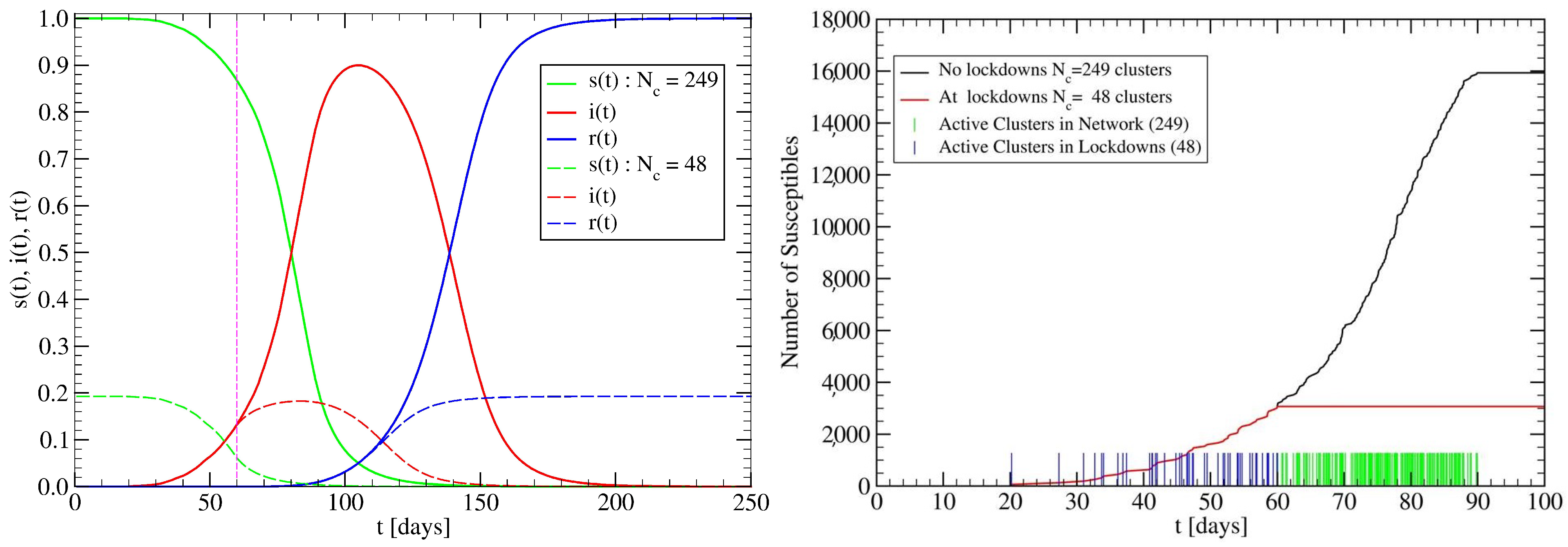
3.2. The Spreading Dynamics on a Network: Effects of Lockdowns

In the following, we illustrate the concept of a network discussed qualitatively in Section 2, with two examples: Without lockdowns, and with lockdowns.

In the case without lockdowns, we consider a network composed of $N_c$ minor (percolation) clusters. We assume that the internal dynamics of each minor cluster has been solved and denote the corresponding solutions as $I_i\left(t\right)$ and $R_i\left(t\right)$, where $1\le i\le N_c$ is the minor cluster index. Denoting by $t_i$ the time at which the infection starts at the ith cluster, the total number of infecteds and recovereds at time t in the network can be written in the form (cf. Equation (1)),

$$\begin{array}{ccc}\hfill I\left(t\right)& =& {\displaystyle \sum _{i=1}^{N_c}}{I}_i(t-t_i)\Theta (t-t_i),\hfill \end{array}$$

(2)

$$\begin{array}{ccc}\hfill R\left(t\right)& =& {\displaystyle \sum _{i=1}^{N_c}}{R}_i(t-t_i)\Theta (t-t_i),\hfill \end{array}$$

(3)

where $\Theta \left(x\right)=1$ for $x\ge 1$ and $\Theta \left(x\right)=0$ otherwise. Each minor cluster has an initial number of susceptibles $N_i$, from which one can obtain the total susceptibles, $S\left(t\right)=N-I\left(t\right)-R\left(t\right)$, where $N={\sum }_{i=1}^{N_c}{N}_i$ is the initial number of susceptibles in the network. An example for $N_c=3$ is shown in Figure 8.

In the case with lockdowns, the latter can be described using a hard cutoff ${\tau }_0$, so that clusters with $t_i>{\tau }_0$ do not become infected, hence do not contribute to the summation in Equations (2) and (3), i.e.,

$$I_{\mathrm{Lock}}\left(t\right)=\sum _{i=1}^{N_c}{I}_i(t-t_i)\Theta (t-t_i)(1-\Theta (t_i-{\tau }_0)),$$

(4)

and similarly for $R_{\mathrm{Lock}}\left(t\right)$. Then, one can calculate $S_{\mathrm{Lock}}\left(t\right)=N_{\mathrm{Lock}}-I_{\mathrm{Lock}}\left(t\right)-R_{\mathrm{Lock}}\left(t\right)$, where $N_{\mathrm{Lock}}={\sum }_{i=1}^{N_c}{N}_i(1-\Theta (t_i-{\tau }_0))$. An example is shown in Figure 9, with $N_c=249$.

To create the network in Figure 9 we use, $\mathsf{\Delta }{N}_c\left(t_c\right)=\mathrm{int}\left[a\right]$, with $a={\tau }_c^{-1}exp(t_c/{\tau }_c)$, ${\tau }_c=9$, and $t_c=1,2,\dots ,50$. For each $t_c$, we generate $1\le j\le \mathsf{\Delta }{N}_c\left(t_c\right)$ times $t_j$, with $t_j=2(t_c-10)+10{\eta }_j$, where $0<{\eta }_j<1$ is a uniformly distributed random number. Afterwards, the times are sorted in ascending order yielding the cluster time lags $t_i$, $20t_0\lesssim t_i\lesssim 90t_0$ (vertical lines), which are used in Equations (2) and (4). Values for $〈R_0〉$ can be read from Table 1.

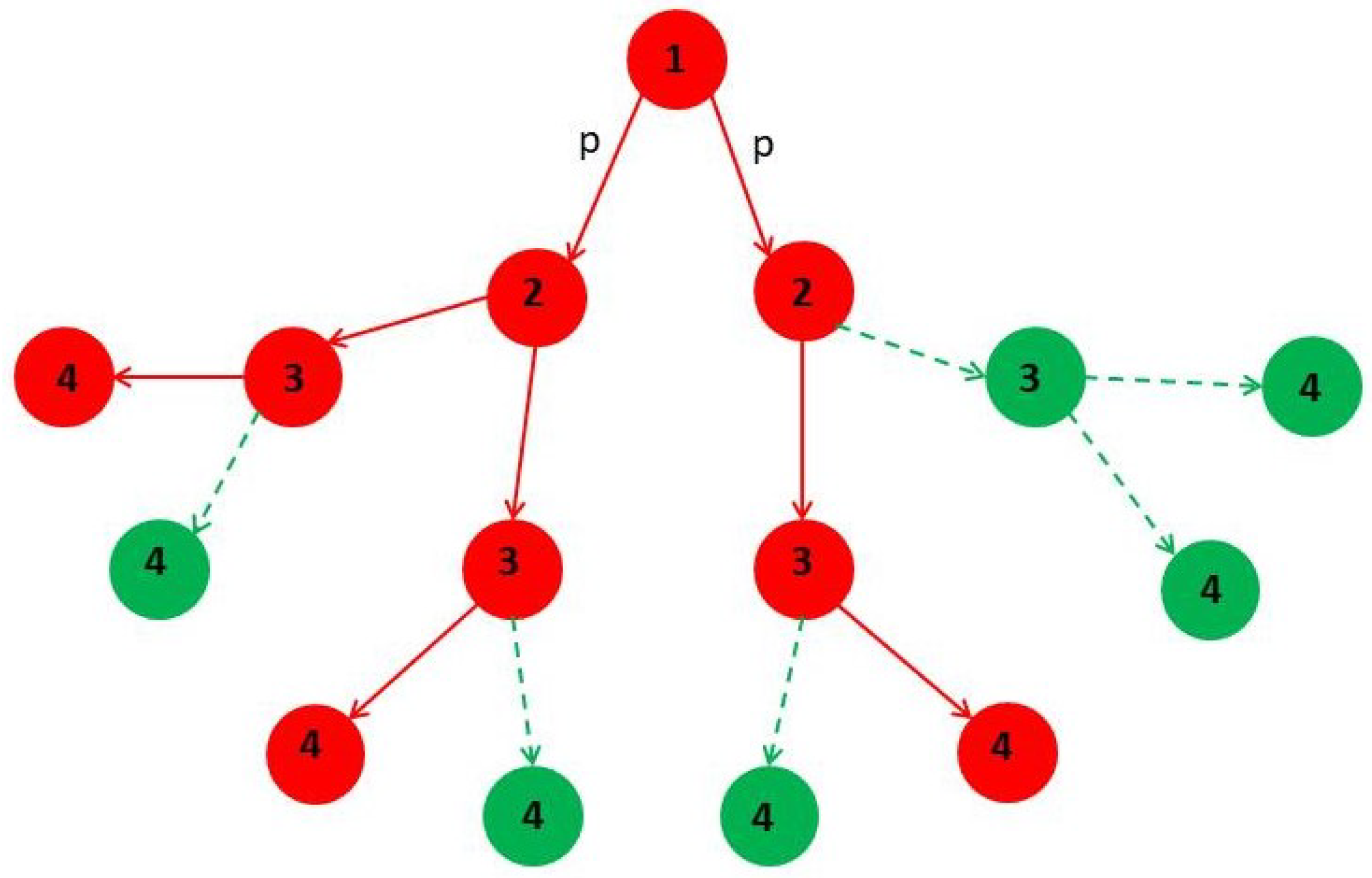
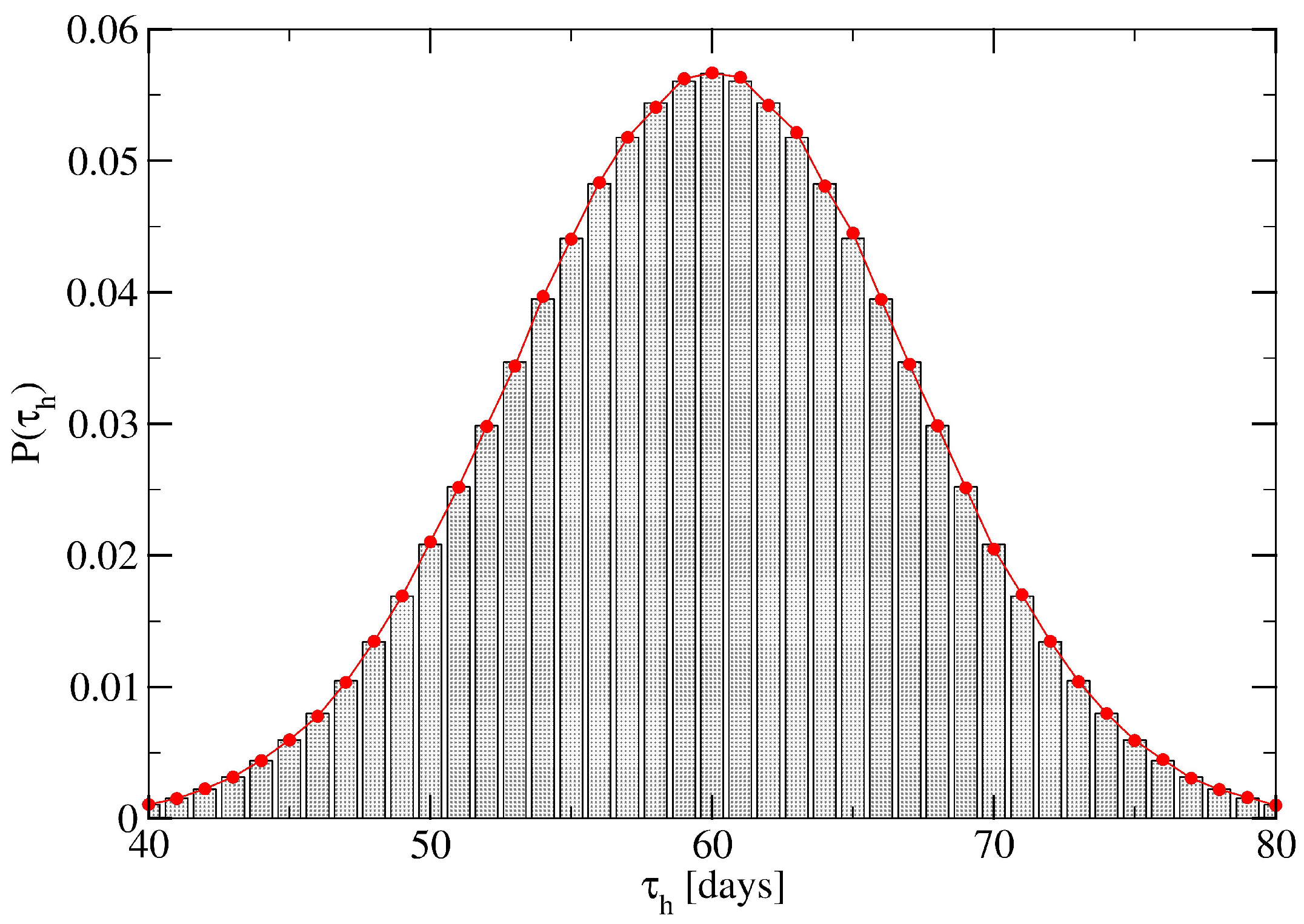
4. Minor Clusters Modeled as Random Trees

Minor percolation clusters discussed in Section 3 do not admit an analytical solution for the spreading of infections. For complex and large population networks, it is clearly most convenient to have analytical solutions for the SIR functions. Following the ideas from the previous section, we discuss a model of a minor cluster which admits an analytical solution. It is based on a directed tree with infection degree z (coordination number or node degree $z+1$), in which the nodes represent susceptibles and the links (edges) effective contacts among them. We consider that initially (time $t=1$) the node at the top of the tree is infected and it can infect a susceptible with a probability p (Figure 10). This means that at most z susceptibles can be infected at time $t=2$, since it has no connections with other members in the cluster. Nodes which are not infected at a given time remain susceptibles forever (see Figure 10). For such a loopless graph, the clustering coefficient of any node vanishes (see e.g., [42]). One can view the tree-like model as a sort of mean-field solution for single percolation clusters, which should yield comparable values of $R_0$.

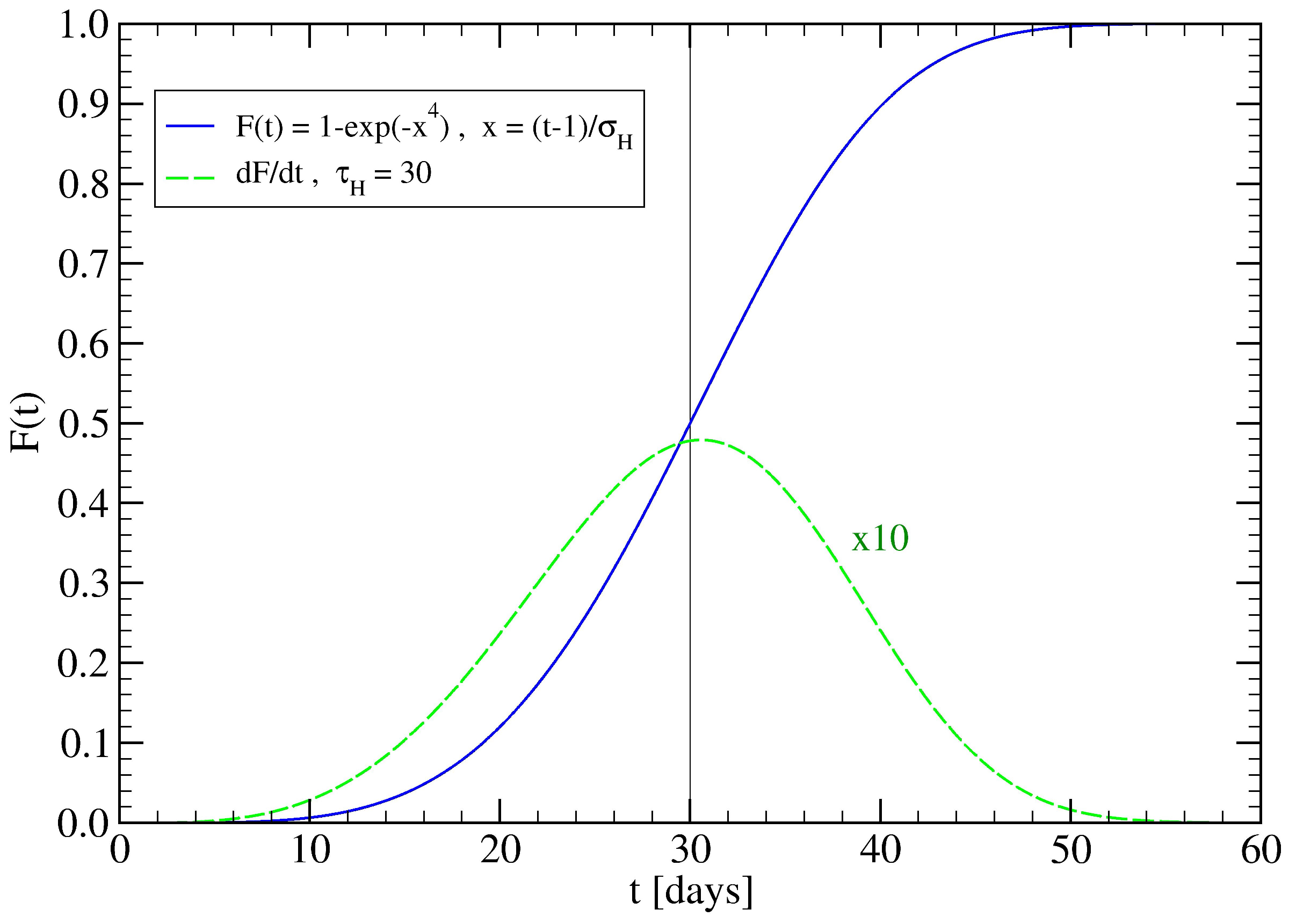
4.1. Effect of Healings Inside a Random Tree

The model described in Figure 10 is incomplete since we need to consider the missing case of recovereds. This means we need to implement a healing process, which is closely related to the issue of contagious period, as we discussed in Section 2. In the case $p=1$, all susceptibles within the tree will be infected, and since we are dealing with a finite population, N, of individuals, we can determine the maximum time T required to infect them all according to the relation,

$$N=\frac{z^T-1}{z-1}.$$

(5)

It is useful to consider a numerical example to elucidate the meaning of the parameter p. If we take say, $z=4$ and $N=2\times {10}^5$, then $T=log(3N+1)/log\left(4\right)\cong 10$ days. Now, let us take say, $p=0.8$. In this case the total infecteds would be $I_0\left(T\right)=[{\left(4p\right)}^T-1]/(4p-1)\cong 5\times {10}^4\approx 0.25N$, which is about one quarter of the total population inside the cluster. The total number of infecteds depends sensitively on the actual value of p, and it appears to play a structural role rather than being directly related to a contagious period. We therefore regard p as a structural parameter, similar to the role played by dormants in the lattice model of infection spreading [9], or the blocked sites in the case of percolation.

To implement a healing mechanism, we assume that an infected can be healed after some amount of time. To make the model a bit more realistic, we do not assume a single healing time, ${\tau }_{\mathrm{H}}$, rather a distribution of them. If we take healing into account, the number of infecteds, $I\left(t\right)$, will decrease in time after reaching its maximum, according to the relation,

$$I\left(t\right)=I_0\left(t\right)-R\left(t\right),$$

(6)

where

$$\begin{array}{ccc}\hfill I_0\left(t\right)& =& \frac{R_0^t-1}{R_0-1},\mathrm{for}t\le T,\mathrm{and}\hfill \end{array}$$

(7)

$$\begin{array}{ccc}\hfill I_0\left(t\right)& =& I_0\left(T\right),\mathrm{for}t>T,\hfill \end{array}$$

(8)

with $R_0=pz$, and $R\left(t\right)$ is total number of recovereds at time t, which can be calculated as,

$$R\left(t\right)=\sum _{t^{\prime }=1}^t\mathsf{\Delta }{I}_0\left(t^{\prime }\right)F(t-t^{\prime }),$$

(9)

where $\mathsf{\Delta }{I}_0\left(t^{\prime }\right)=R_0^{t^{\prime }-1}$, for $t^{\prime }\le T$, and $\mathsf{\Delta }{I}_0\left(t^{\prime }\right)=0$, for $t^{\prime }>T$, while $F\left(x\right)$ is a smooth increasing function of $x=t-t^{\prime }$, such as

$$\begin{array}{ccc}\hfill F\left(x\right)& =& 1-exp\left[-{(x-1)}^4/{\sigma }_{\mathrm{H}}^4\right],\mathrm{for}x\ge 1,\hfill \end{array}$$

(10)

$$\begin{array}{ccc}\hfill F\left(x\right)& =& 0,\mathrm{otherwise}.\hfill \end{array}$$

(11)

An example is displayed in Figure 11. Using this form for $F\left(x\right)$ into Equation (9), one obtains a smoothly growing recovereds curve.

Finally, the total number of susceptibles can be obtained from the (conservation number) sum rule, $S\left(t\right)+I\left(t\right)+R\left(t\right)=N$, yielding,

$$S\left(t\right)=N-I_0\left(t\right),\mathrm{for}t\le T,$$

(12)

with $S\left(t\right)=N-I_0\left(T\right)$, for $t>T$. An example of how Equations (6), (9) and (12) actually work is shown in Figure 12.

4.2. Effect of Lockdowns Inside a Random Tree without Healings

In some cases, in particular for large clusters, one would like to describe the effects of lockdowns, or distancing, inside a minor cluster. To model the effects of lockdowns, we assume that the reproduction number $R_0$ (Figure 10) decreases with time t. In other words, the effect of ‘distancing’ can be interpreted as effectively reducing $R_0$. In order to assess the effects of lockdowns in a way that can be treated analytically, and thus being useful for the applications, we consider a specific model in which $R_0$ depends on time according to (see also [8]),

$$\begin{array}{ccc}\hfill R_0& =& pz,\mathrm{for}t\le \tau -1,\hfill \end{array}$$

(13)

$$\begin{array}{ccc}\hfill R_0\left(t\right)& =& R_0{e}^{-(t-\tau )/{\tau }_q},\mathrm{for}t\ge \tau ,\hfill \end{array}$$

(14)

where $\tau$ is the time lag after which the lockdowns effectively start, and ${\tau }_q>0$ is the quarantine reaction time parameter. Clearly, one must have $\tau <T$ for the quarantine to have an effect. Please note that when ${\tau }_q\to \infty$, we recover the exponential growth model described in Figure 10. Actually, ${\tau }_q\lesssim 1$ to be efficient, since its inverse, $1/{\tau }_q$ represents the reaction speed of the lockdowns to new transmissions.

According to Equation (13), the number of new infections at times $t\le \tau -1$, is given by $\mathsf{\Delta }{I}_0\left(t\right)=R_0^{t-1}$, and the total number of infections will simply be,

$$I_0\left(t\right)=\frac{R_0^t-1}{R_0-1},\mathrm{for}t\le \tau -1,$$

(15)

as in Equation (7), while for $t\ge \tau$, we have

$$I_0\left(t\right)=I_0(\tau -1)+\sum _{t^{\prime }=0}^{t-\tau }\mathsf{\Delta }{I}_q\left(t^{\prime }\right),\mathrm{for}t\ge \tau .$$

(16)

Let us calculate $\mathsf{\Delta }{I}_q\left(t^{\prime }\right)$ recursively, and for simplicity of notation we define $b=exp(-1/{\tau }_q)$, where $0<b\le 1$. We find,

$$\begin{array}{ccc}\hfill \mathsf{\Delta }{I}_q\left(0\right)& =& R_0^{\tau -1},\hfill \\ \hfill \mathsf{\Delta }{I}_q\left(1\right)& =& \mathsf{\Delta }{I}_q\left(0\right)R_{0}b=R_0^{\tau -1}{R}_{0}b,\hfill \\ \hfill \mathsf{\Delta }{I}_q\left(2\right)& =& \mathsf{\Delta }{I}_q\left(1\right)R_0^2{b}^2=R_0^{\tau -1}{R}_0^{2}b{b}^2,\hfill \\ \hfill \mathsf{\Delta }{I}_q\left(3\right)& =& \mathsf{\Delta }{I}_q\left(2\right)R_0^3{b}^3=R_0^{\tau -1}{R}_0^{3}b{b}^2{b}^3,\hfill \\ & \cdots & \hfill \\ \hfill \mathsf{\Delta }{I}_q\left(t^{\prime }\right)& =& \mathsf{\Delta }{I}_q(t^{\prime }-1)R_0^{t^{\prime }}{b}^{t^{\prime }}=R_0^{\tau -1}{R}_0^{t^{\prime }}{b}^{t^{\prime }(t^{\prime }+1)/2}.\hfill \end{array}$$

To be noted is that $\mathsf{\Delta }{I}_q\left(t^{\prime }\right)\le R_0^{T-1}$ for $\tau \le T$, so that the upper time T does not play a role in this case. We can now rewrite Equation (16) in the more convenient form, valid for $t\ge \tau$,

$$I_0\left(t\right)=I_0(\tau -1)+R_0^{\tau -1}\sum _{t^{\prime }=0}^{t-\tau }{R}_0^{t^{\prime }}{b}^{t^{\prime }/2}{b}^{{t^{\prime }}^2/2}.$$

(17)

Using the relation ${\sum }_{j=0}^m{R}_0^j=(R_0^{m+1}-1)/(R_0-1)$, it can be easily verified that Equation (17) reduces to the standard case when $b=1$ (Figure 10). To be noted is that in the hypothetical limit $b\to 0$ (i.e., ${\tau }_q\to 0$), the total infections stop at,

$$I_0\left(\tau \right)=(R_0^{\tau }-1)/(R_0-1)\le I_0\left(T\right).$$

(18)

In the general case, $0<b<1$, the total number of infecteds can be estimated analytically. To this end, we transform the sum over $t^{\prime }$ in Equation (17), into an integral over a continuous variable t, using the exact relation,

$$R_0^t{b}^{t/2}{b}^{t^2/2}=exp\left(A\right),A=tlog{R}_0+\frac{t}{2}logb+\frac{t^2}{2}logb.$$

(19)

Completing the square in the expression for A, we find,

$$A=-\frac{1}{2{\tau }_q}{(t-\gamma )}^2+\frac{{\gamma }^2}{2{\tau }_q},$$

(20)

where $\gamma ={\tau }_{q}log{R}_0-1/2$. We can now evaluate the integral,

$$\begin{array}{ccc}\hfill G(R_0,{\tau }_q)& =& {\int }_0^{\infty }dt{e}^A=a{e}^{{(\gamma /a)}^2}{\int }_0^{\infty }dx{e}^{-{(x-\gamma /a)}^2}\hfill \\ & =& {\left(\frac{\pi {\tau }_q}{2}\right)}^{1/2}{e}^{{(\gamma /a)}^2}[\mathrm{erf}(\gamma /a)+1],\hfill \end{array}$$

(21)

where $a=\sqrt{2{\tau }_q}$. We can use the value $2{\tau }_0=1/log{R}_0$, for which $\gamma =0$, to write,

$$\gamma /a=\frac{1}{\sqrt{8{\tau }_q}}\frac{({\tau }_q-{\tau }_0)}{{\tau }_0}.$$

(22)

Let us consider the behavior of $G(R_0,{\tau }_q)$ in the limits ${\tau }_q\to \infty$ and ${\tau }_q\to 0$.

• ${\tau }_q\to \infty$: In this case, $x=\gamma /a\cong \sqrt{{\tau }_q/2}log{R}_0$, and using the asymptotic expansion, $\mathrm{erf}\left(x\right)\cong 1-{\left(\sqrt{\pi x^2}\right)}^{-1}exp(-x^2)$, for $x\gg 1$, yields $G(R_0,{\tau }_q)\cong {\left(2\pi {\tau }_q\right)}^{1/2}{R}_0^{({\tau }_q/2)log{R}_0}$$\to \infty$, consistent with $I_0(\infty )\to \infty$ when $R_0>1$ and $T\to \infty$.
• ${\tau }_q\to 0$: In this case, $x=-1/\sqrt{8{\tau }_q}\to -\infty$ and $\mathrm{erf}\left(x\right)\cong -1+{\left(\sqrt{\pi x^2}\right)}^{-1}exp(-x^2)$, yielding $G(R_0,{\tau }_q)\cong 2{\tau }_q\to 0$, consistent with the stop of infection spreading at time $\tau$.

We can now evaluate the total number of infecteds, $I_0\left(t\right)$, from Equation (17) when $t\to \infty$, which we denote as $I_{\infty }(R_0,\tau ,{\tau }_q)$, using Equation (21), yielding

$$I_{\infty }(R_0,\tau ,{\tau }_q)=\frac{R_0^{\tau -1}-1}{R_0-1}+R_0^{\tau -1}G(R_0,{\tau }_q).$$

(23)

Let us consider first the case $R_0=1$ (yielding ${\tau }_0\to \infty$). We find, $I_{\infty }(1,\tau ,{\tau }_q)=\tau -1+G(1,{\tau }_q)$, where

$$G(1,{\tau }_q)={\left(\frac{\pi {\tau }_q}{2}\right)}^{1/2}{e}^{1/8{\tau }_q}\left(\mathrm{erf}\left(-1/\sqrt{8{\tau }_q}\right)+1\right).$$

(24)

As an example, let us take ${\tau }_q=10$. Then, $G(1,10)\cong 3.5$, and using this into Equation (23), yields, $I_{\infty }(1,\tau ,10)=\tau -1+G(1,10)\cong \tau +2.5$. In the case ${\tau }_q\ll 1$, we then find, $G(1,{\tau }_q)=2{\tau }_q$, thus, $I_{\infty }(1,\tau ,{\tau }_q)=\tau -1+2{\tau }_q\cong \tau -1$.

Another special case is the one corresponding to $\gamma =0$, where $\mathrm{erf}\left(0\right)=0$. In this case we have ${\tau }_q={\tau }_0$, with

$${\tau }_q=\frac{1}{log{R}_0^2},\mathrm{and}G(R_0,{\tau }_0)={\left(\frac{\pi }{4log{R}_0}\right)}^{1/2}.$$

(25)

If for this case, we take $R_0=1+\epsilon$, with $0<\epsilon \ll 1$, then ${\tau }_0\cong (1/2){(R_0-1)}^{-1}\gg 1$, and, as a result, $G(R_0,{\tau }_0)\cong \sqrt{\pi /4}{(R_0-1)}^{-1/2}\gg 1$. To be efficient, quarantines should act on times scales ${\tau }_q<{\tau }_0$. This can be the case also in the presence of sufficiently slow healing processes (see Section 4.3). According to Equation (25), we can estimate the upper bounds ${\tau }_0$ for efficient lockdowns. We find, for example for $R_0=1.1$, that ${\tau }_q<5$ days; while for $R_0=4$, ${\tau }_q<0.17$ days $\sim 4$ h, suggesting that lockdowns should be ‘faster’ enough to prevent new infections taking place at a rate of one every 4 h.

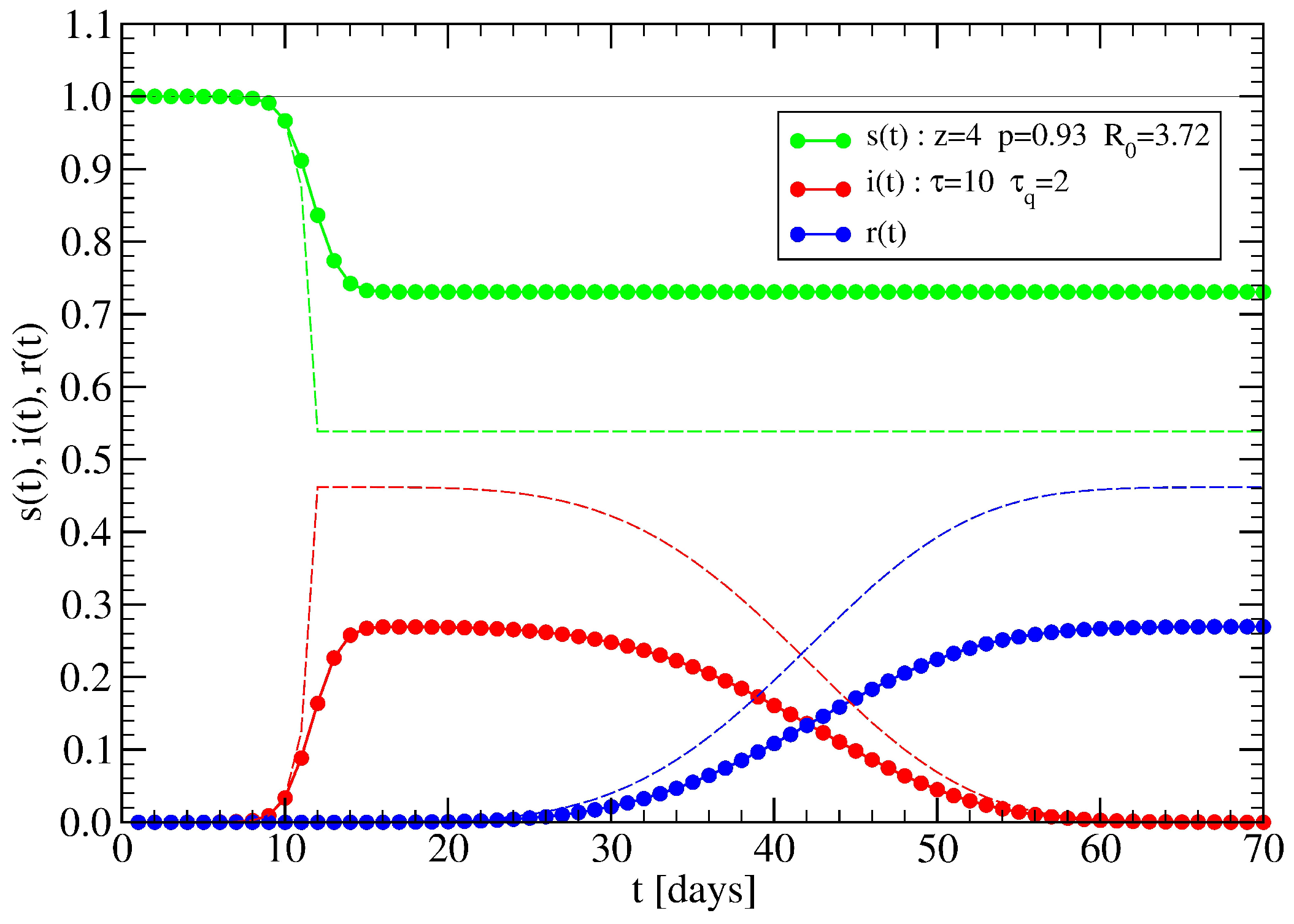
4.3. Effect of Lockdowns Inside a Random Tree with Healings

Next, we consider both lockdown and healing effects together. For the former, we assume $\tau <T$, meaning that lockdowns start acting before the whole population has been infected. In this case, T does not play a role in the process (cf. Section 4.2). The corresponding relations for $I\left(t\right)$, $R\left(t\right)$ and $S\left(t\right)$, now become,

$$I\left(t\right)=I_0\left(t\right)-R\left(t\right),$$

(26)

where

$$\begin{array}{ccc}\hfill I_0\left(t\right)& =& \frac{R_0^t-1}{R_0-1},\mathrm{for}t\le \tau -1,\mathrm{and}\hfill \end{array}$$

(27)

$$\begin{array}{ccc}\hfill I_0\left(t\right)& =& I_0(\tau -1)+{\displaystyle \sum _{t^{\prime }=0}^{t-\tau }}\mathsf{\Delta }{I}_q\left(t^{\prime }\right),\mathrm{for}t\ge \tau ,\hfill \end{array}$$

(28)

where $\mathsf{\Delta }{I}_q\left(t^{\prime }\right)=R_0^{\tau -1}{R}_0^{t^{\prime }}{e}^{-t^{\prime }(t^{\prime }+1)/2{\tau }_q}$, and

$$R\left(t\right)=\sum _{t^{\prime }=1}^t\mathsf{\Delta }{I}_q\left(t^{\prime }\right)F(t-t^{\prime }),$$

(29)

with

$$\begin{array}{ccc}\hfill \mathsf{\Delta }{I}_q\left(t^{\prime }\right)& =& R_0^{t^{\prime }-1},\mathrm{for}{t}^{\prime }\le \tau -1,\hfill \\ \hfill \mathsf{\Delta }{I}_q\left(t^{\prime }\right)& =& R_0^{t^{\prime }-1}{e}^{-(t^{\prime }-\tau )(t^{\prime }-\tau +1)/2{\tau }_q},\mathrm{for}{t}^{\prime }\ge \tau .\hfill \end{array}$$

Finally, the total number of susceptibles, $S\left(t\right)$, is given by,

$$S\left(t\right)=N-I\left(t\right)-R\left(t\right)=N-I_0\left(t\right),$$

(30)

where $I_0\left(t\right)$ can be obtained from Equations (27) and (28). An illustrative example is shown in Figure 13.

As we can see from Figure 13, the combined effects of both lockdowns and healing result in smoother time dependences of susceptibles and infecteds curves, thus making the model more realistic. A summary of the parameters entering the random tree model is displayed in

Table 2. The set of parameters and main quantities entering the random tree model of minor clusters. The unit of time is $t_0=1$ day.

z	Infection degree	$z\ge 1$
p	Transmission probability	$0<p\le 1$
$R_0$	Reproduction number	$R_0=pz$
N	Total population in cluster	$N=(z^T-1)/(z-1)$
T	Cluster infection time	$T>t_0$
${\tau }_{\mathrm{H}}$	Characteristic healing time	${\tau }_{\mathrm{H}}>t_0$
${\sigma }_{\mathrm{H}}$	Width of $F\left({\tau }_{\mathrm{H}}\right)$	${\sigma }_{\mathrm{H}}=({\tau }_{\mathrm{H}}-1)/{(log2)}^{1/4}$
$\tau$	Lockdown starting time	$\tau >t_0$
${\tau }_q$	Quarantine reaction time	${\tau }_q>0$
$R_0\left(t\right)$	Effective $R_0$ (lockdowns)	$R_0\left(t\right)=R_0{e}^{-(t-\tau )/{\tau }_q}$
${\tau }_0$	Reference reaction time	${\tau }_0=1/(2log{R}_0)$

.

More important, however, is the possibility of considering these random trees as the building blocks of networks on larger scales. Clearly, the fact that one has an analytical solution for achieving the latter goal makes this random tree model amenable for applications. We apply these results to the USA COVID-19 data in the following section.

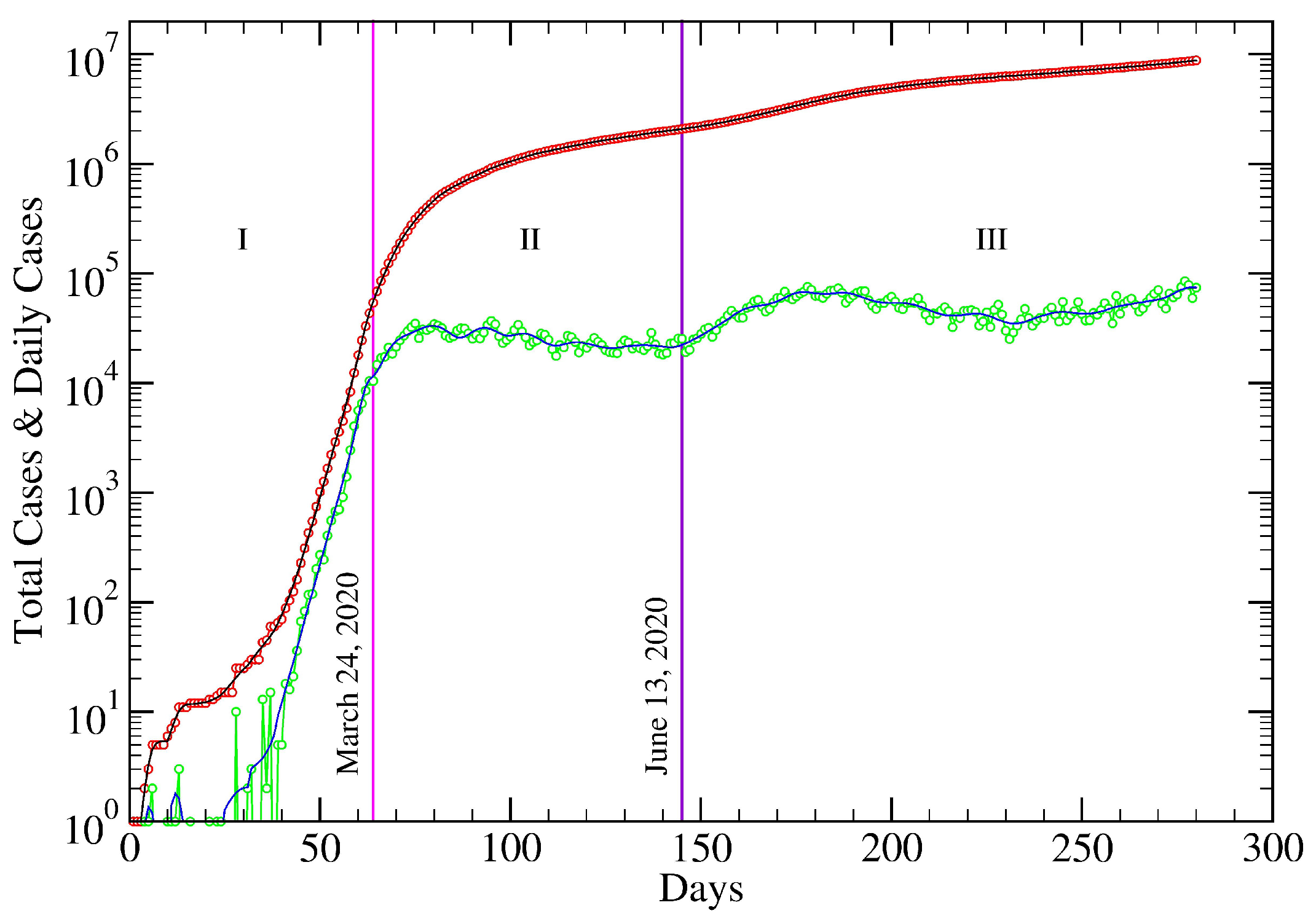
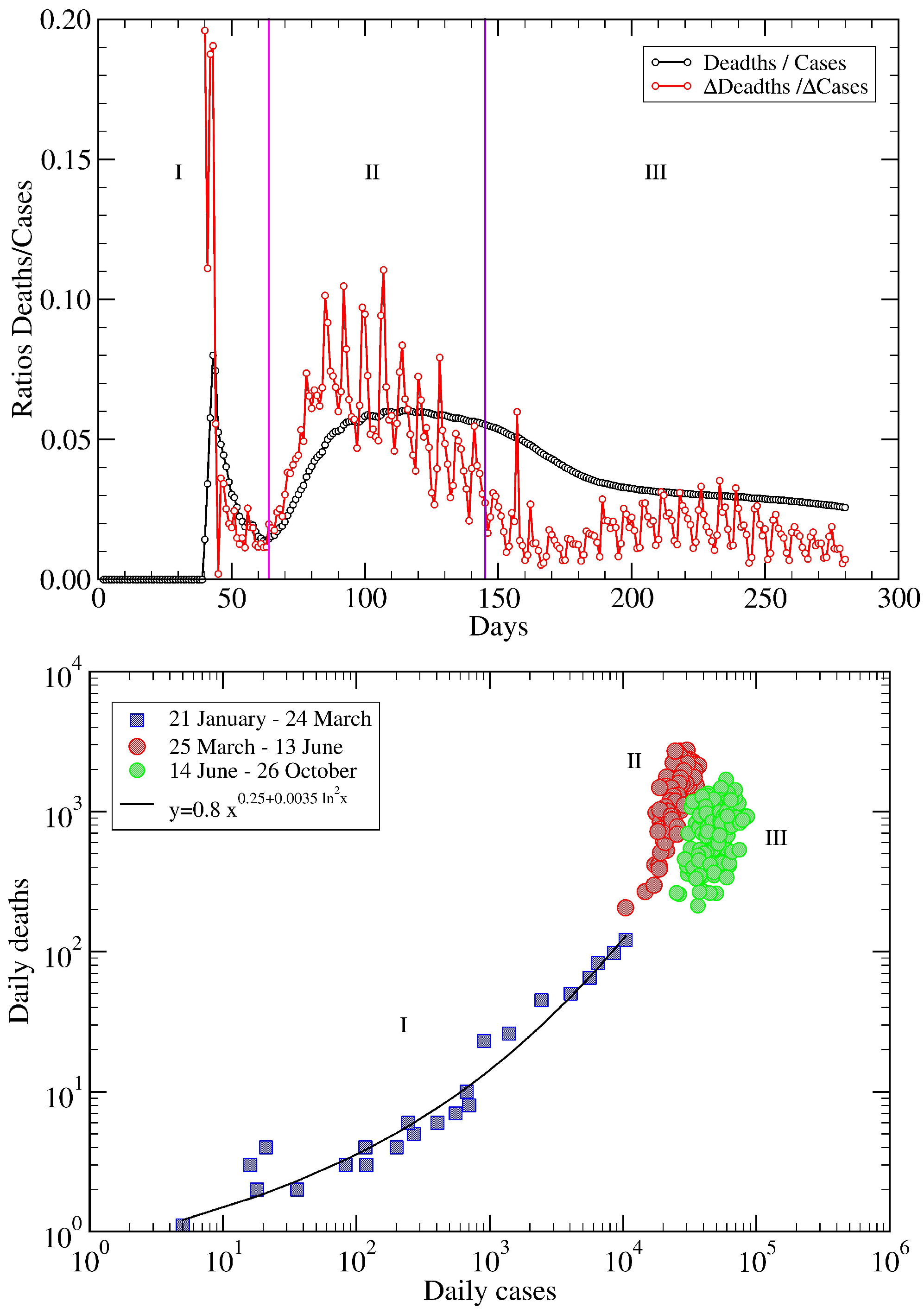
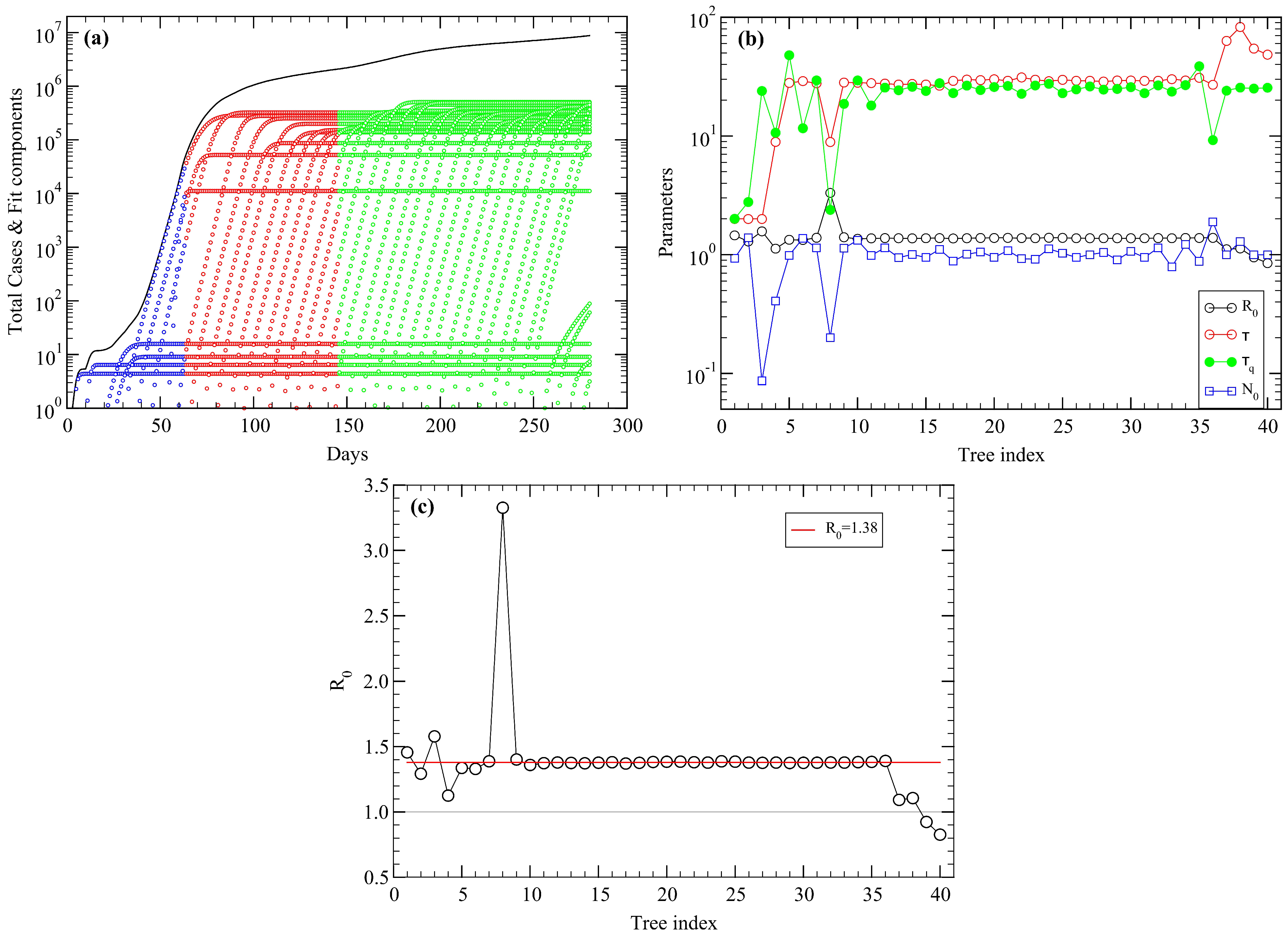
5. USA COVID-19 Data Revisited

As an application of the network ideas discussed above, we consider COVID-19 data from the USA, https://www.worldometers.info/coronavirus/country/us/ (accessed on 26 October 2020), within the period (21 January–26 October 2020). The total cases are plotted in Figure 14 as a function of days. We implemented a fitting procedure using the results from Section 4.3, as described in detail in the Appendix A. The result of the fit is represented by the continuous line in the figure, being almost indistinguishable from the empirical data. These results illustrate the potential usefulness of the cluster method in complex territorial environments spanning both large space and temporal scales.

We then calculated the daily cases, as successive variations of the total cases, which are shown by the green circles (real data) and continuous blue line (fit). The weekly oscillations observed in the real data are reproduced to some extent. To be noted is that the total number of data points is 280, while for the fit we used 40 tree-like clusters with 4 free parameters each, yielding a total of 160 unknown values (see Appendix A for details). The obtained parameters show a remarkable constancy within a period of about six months starting at the end of March 2020. The reproduction number, $R_0\simeq 1.38$, is quite large indeed, and the lockdown parameters, $\tau$ and ${\tau }_q$, span a time scale of about a month.

In Figure 14, we have distinguished three periods within the data which were suggested by the following analysis. To show this, it is interesting to look at the ratios between deaths and cases, both for the total ones and for the daily variations, as illustrated in Figure 15. A close inspection of the data suggests the identification of three different periods during the infection spreading. The first one ends around 24 March, the second one ends around 13 June, and the last one extends until the end of the data. To make the difference clearer, we have depicted the corresponding values with different colors, as shown in the lower panel of Figure 15.

6. Conclusions

We have presented a general network model of a population built upon random finite clusters, representing highly correlated individuals belonging to a social group or community. We study the spreading dynamics of an infectious disease within such a network, characterized by the existence of different times scales for its transmission. The shortest time scales are those within a cluster, while they may be longer within different clusters or communities, reflecting the transmission of infection between two individuals, one infected and one susceptible, belonging to different communities who meet somewhere and stay close enough for some time. We presented results on clusters constructed using percolation concepts, in particular on square lattices below the critical concentration, and on random trees which are amenable of analytical solutions. The SIR variables are obtained as a function of time and both healing and lockdown mechanisms are implemented. We argue that such network models can become very useful to study the spreading of a disease in a population, complementing the widely used SIR system of differential equations, by incorporating the effect of correlations within a cluster or community of susceptible individuals. We applied a simple fitting scheme, based on random trees, to study the temporal evolution of COVID-19 cases in the USA. The results suggest that infections in the country developed with a seemingly constant reproduction number, $R_0\simeq 1.38$, over a period of about six months starting around the end of March 2020. The lockdowns appear to have taken long times (about a month) to have some effect. In future work, one can consider the possibility of incorporating additional parameters into the model, such as community size distributions, contact correlations between communities for infection spreading, etc., in order to extract important and otherwise unknown information regarding the internal structure of a population.

References

1. Dong, E.; Du, H.; Gardner, L. An interactive web-based dashboard to track COVID-19 in real time. Lancet Infect. Dis. 2020, 20, 533–534. [Google Scholar] [CrossRef]
2. Xu, Z.; Shi, L.; Wang, Y.; Zhang, J.; Huang, L.; Zhang, C.; Liu, S.; Zhao, P.; Liu, H.; Zhu, L.; et al. Pathological findings of COVID-19 associated with acute respiratory distress syndrome. Lancet Respir. Med. 2020, 8, 420–422. [Google Scholar] [CrossRef]
3. Fernández-Villaverde, J.; Jones, C.I. Estimating and Simulating a SIRD Model of COVID-19 for Many Countries, States, and Cities. Natl. Bur. Econ. Res. Work. Pap. Ser. 2020, 27, 128. [Google Scholar]
4. Chen, Y.C.; Lu, P.E.; Chang, C.S.; Liu, T.H. A Time-dependent SIR model for COVID-19 with Undetectable Infected Persons. IEEE Trans. Netw. Sci. Eng. 2020, 7, 3279–3294. [Google Scholar] [CrossRef]
5. Wu, J.T.; Leung, K.; Bushman, M.; Kishore, N.; Niehus, R.; de Salazar, P.M.; Cowling, B.J.; Lipsitch, M.; Leung, G.M. Estimating clinical severity of COVID-19 from the transmission dynamics in Wuhan, China. Nat. Med. 2020, 26, 506–510. [Google Scholar] [CrossRef] [Green Version]
6. Yang, Z.; Zeng, Z.; Wang, K.; Wong, S.S.; Liang, W.; Zanin, M.; Liu, P.; Cao, X.; Gao, Z.; Mai, Z.; et al. Modified SEIR and AI prediction of the epidemics trend of covid-19 in China under public health interventions. J. Thorac. Dis. 2020, 12, 165. [Google Scholar] [CrossRef]
7. Chinazzi, M.; Davis, J.T.; Ajelli, M.; Gioannini, C.; Litvinova, M.; Merler, S.; Piontti, A.P.; Mu, K.; Rossi, L.; Sun, K.; et al. The effect of travel restrictions on the spread of the 2019 novel coronavirus (COVID-19) outbreak. Science 2020, 368, 395–400. [Google Scholar] [CrossRef] [Green Version]
8. Palladino, A.; Nardelli, V.; Atzeni, L.G.; Cantatore, N.; Cataldo, M.; Croccolo, F.; Estrada, N.; Tombolini, A. Modelling the spread of Covid19 in Italy using a revised version of the SIR model. arXiv 2020, arXiv:2005.08724. [Google Scholar]
9. Croccolo, F.; Roman, H.E. Spreading of infections on random graphs: A percolation-type model for COVID-19. Chaos Solitons Fractals 2020, 139, 110077. [Google Scholar] [CrossRef]
10. Kermack, W.O.; McKendrick, A.G. A Contribution to the Mathematical Theory of Epidemics. Proc. R. Soc. Lond. Ser. A 1927, 115, 700–721. [Google Scholar]
11. Hethcote, H.W. The Mathematics of Infectious Diseases. SIAM Rev. 2000, 42, 599–653. [Google Scholar] [CrossRef] [Green Version]
12. Chen, D. Modeling the spread of infectious diseases: A review. In Analyzing and Modeling Spatial and Temporal Dynamics of Infectious Diseases; Chen, D., Moulin, B., Wu, J., Eds.; John Wiley & Sons: Hoboken, NJ, USA, 2014; pp. 19–42. [Google Scholar]
13. Bailey, N.T.J. The Mathematical Theory of Epidemics, 1st ed.; Charles Griffin & Company: London, UK, 1957. [Google Scholar]
14. Anderson, R.M.; May, R.M. Infectious Diseases of Humans: Dynamics and Control; Oxford University Press: Oxford, UK, 1991; Volume 757. [Google Scholar]
15. Fraser, C.; Riley, S.; Anderson, R.M.; Ferguson, N.M. Factors that make an infectious disease outbreak controllable. Proc. Natl. Acad. Sci. USA 2004, 101, 6146–6151. [Google Scholar] [CrossRef] [PubMed] [Green Version]
16. Pellis, L.; Ball, F.; Trapman, P. Reproduction numbers for epidemic models with households and other social structures. I. Definition and calculation of R0. Math. Biosci. 2012, 235, 85–97. [Google Scholar] [CrossRef] [PubMed]
17. Ben-Avraham, D.; Havlin, S. Diffusion and Reactions in Fractals and Disordered Systems; Cambridge University Press: Cambridge, UK, 2000. [Google Scholar]
18. Bunde, A.; Havlin, S. Fractals and Disordered Systems; Springer Science & Business Media: Berlin/Heidelberg, Germany, 2012. [Google Scholar]
19. Stauffer, D.; Aharony, A. Introduction to Percolation Theory; Taylor & Francis: London, UK, 2018. [Google Scholar]
20. Matouk, A.E. Complex dynamics in susceptible-infected models for COVID-19 with multi-drug resistance. Chaos Solitons Fractals 2020, 140, 110257. [Google Scholar] [CrossRef] [PubMed]
21. Moussaoui, A.; Zerga, E.H. Transmission dynamics of COVID-19 in Algeria: The impact of physical distancing and face masks. AIMS Public Health 2020, 7, 816. [Google Scholar] [CrossRef]
22. Kasinathan, P.; Montoya, O.D.; Gil-González, W.; Arul, R.; Moovendan, M.; Dhivya, S.; Kanimozhi, R.; Angalaeswari, S. Application of soft computing techniques in the analysis of COVID-19: A Review. Eur. J. Mol. Clin. Med. 2020, 7, 2480–2503. [Google Scholar]
23. Tuteja, G.S. Stability and Numerical Investigation of modified SEIR model with Vaccination and Life-long Immunity. Eur. J. Mol. Clin. Med. 2020, 7, 3034–3044. [Google Scholar]
24. Manríquez, R.; Guerrero-Nancuante, C.; Martínez, F.; Taramasco, C. Spread of Epidemic Disease on Edge-weighted Graphs from a Database: A Case Study of COVID-19. Int. J. Environ. Res. Public Health 2021, 18, 4432. [Google Scholar] [CrossRef]
25. Czypionka, T.; Greenhalgh, T.; Bassler, D.; Bryant, M.B. Masks and face coverings for the lay public: A narrative update. Ann. Intern. Med. 2021, 174, 511–520. [Google Scholar] [CrossRef]
26. Frank, T.D. Simplicity From Complexity: On The Simple Amplitude Dynamics Underlying Covid-19 Outbreaks In China. Adv. Complex Syst. 2021, 23, 2050022. [Google Scholar] [CrossRef]
27. Schlickeiser, R.; Kröger, M. Analytical solution of the SIR-model for the temporal evolution of epidemics: Part B. Semi-time case. J. Phys. A Math. Theor. 2021, 54, 175601. [Google Scholar] [CrossRef]
28. Ramaswamy, H.; Oberai, A.A.; Yortsos, Y.C. A comprehensive spatial-temporal infection model. Chem. Eng. Sci. 2021, 233, 116347. [Google Scholar] [CrossRef] [PubMed]
29. Hemmer, C.J.; Hufert, F.; Siewert, S.; Reisinger, E. Protection from COVID-19: The efficacy of face masks. Dtsch. Ärztebl. Int. 2021, 118, 59. [Google Scholar] [CrossRef] [PubMed]
30. Dogan, O.; Tiwari, S.; Jabbar, M.A.; Guggari, S. A systematic review on AI/ML approaches against COVID-19 outbreak. Complex Intell. Syst. 2021, 7, 2655–2678. [Google Scholar] [CrossRef] [PubMed]
31. Huang, B.; Yang, J.X.; Li, X. Identifying influential links to control spreading of epidemics. Phys. A Stat. Mech. Its Appl. 2021, 583, 126291. [Google Scholar] [CrossRef]
32. Pavan Kumar, S.T.; Lahiri, B.; Alvarado, R. Multiple change point estimation of trends in Covid-19 infections and deaths in India as compared with WHO regions. Spat. Stat. 2021, 44, 100538. [Google Scholar]
33. Buzea, C.G.; Eva, L.; Prelipceanu, M.; Cazacu, M.M.; Garofalide, S.; Agop, M. Coronavirus disease COVID-19 tracking the global outbreak. SEIR compartmental model applied to SARS-CoV-2 epidemic in Romania. In Biomedical Engineering Tools for Management for Patients with COVID-19; Elsevier: Amsterdam, The Netherlands, 2021; pp. 87–102. [Google Scholar]
34. Kröger, M.; Schlickeiser, R. Verification of the accuracy of the SIR model in forecasting based on the improved SIR model with a constant ratio of recovery to infection rate by comparing with monitored second wave data. R. Soc. Open Sci. 2021, 8, 211379. [Google Scholar] [CrossRef]
35. Gandzha, I.S.; Kliushnichenko, O.V.; Lukyanets, S.P. Modeling and controlling the spread of epidemic with various social and economic scenarios. Chaos Solitons Fractals 2021, 148, 111046. [Google Scholar] [CrossRef]
36. Barthélemy, M.; Barrat, A.; Pastor-Satorras, R.; Vespignani, A. Dynamical patterns of epidemic outbreaks in complex heterogeneous networks. J. Theor. Biol. 2005, 235, 275–288. [Google Scholar] [CrossRef] [Green Version]
37. Colizza, V.; Vespignani, A. Invasion Threshold in Heterogeneous Metapopulation Networks. Phys. Rev. Lett. 2007, 99, 148701. [Google Scholar] [CrossRef] [Green Version]
38. Shao, Q.; Han, D. Epidemic spreading in metapopulation networks with heterogeneous mobility rates. Appl. Math. Comput. 2022, 412, 126559. [Google Scholar] [CrossRef]
39. Kraemer, M.U.G.; Yang, C.H.; Gutierrez, B.; Wu, C.H.; Klein, B.; Pigott, D.M.; Open COVID-19 Data Working Group; du Plessis, L.; Faria, N.R.; Li, R.; et al. The effect of human mobility and control measures on the COVID-19 epidemic in China. Science 2020, 368, 493–497. [Google Scholar] [CrossRef] [PubMed] [Green Version]
40. Ordemann, A.; Roman, H.E.; Bunde, A. Cluster growth at the percolation threshold with a finite lifetime of growth sites. Phys. A Stat. Mech. Appl. 1999, 266, 92–95. [Google Scholar] [CrossRef]
41. Roman, H.E. Diffusion in three-dimensional random systems at their percolation thresholds. J. Stat. Phys. 1990, 58, 375–382. [Google Scholar] [CrossRef]
42. Bollobás, B. Modern Graph Theory; Springer Science & Business Media: Berlin/Heidelberg, Germany, 2013; Volume 184. [Google Scholar]
Figure 1. Illustration of the lattice percolation model for the spreading of an infectious disease in a population [9], for the case of nearest neighbor (NN) site percolation at concentration p = 1 / 2 . For the latter, initially half of the sites represent susceptible individuals (green squares), and the other half dormant (inactive) ones (black squares). Susceptibles do not interact with dormants, i.e., the disease can only be transmitted to a susceptible. NN sites of similar category (either green or black squares) form a cluster. As an example, the stars indicate the largest cluster of susceptibles within this portion of the lattice, while the open circles the ‘isolated’ clusters of single susceptibles. For this value of p, all clusters are finite in the sense that they do not ‘percolate’ the lattice. In the model, new connections among susceptibles can develop dynamically (in the absence of lockdowns), allowing for the spreading of the disease among different clusters. The transmission of infection is the fastest among NN sites, while becoming less likely among different clusters, leading to different time scales for spreading. As we will see, another choice such as site percolation in 3d is not so convenient. Therefore, we stick at 2d site percolation.
Mathematics 09 03054 g001
Figure 2. Scheme of a cluster network model for spreading disease. A population of susceptible individuals is organized into ‘major’ clusters (blue circles, labelled with numbers), which in turn are composed of smaller ‘minor’ clusters (white circles, labelled with letters). The largest major cluster in this example is No. 3, composed of 5 minor clusters. The infection starts at the top minor cluster (red circle) within cluster No. 1. Infection spreads the fastest inside minor clusters, on time scales denoted as say, τ a , a , and proceed to neighbor minor clusters on longer times scales, τ a , b > τ a , a τ b , b (see e.g., cluster No. 2). At even longer time scales, infection can extend among major clusters, such as τ 1 , 2 τ a , b . The dashed lines indicate transmission paths which have been blocked by lockdowns, thus avoiding further spreading of infections among the remaining, here No. (6–11), major clusters. On larger population scales, the above set of 11 major clusters can be seen as a ‘super-cluster’, representing just a minor part of a larger agglomeration, such as a city or a country.
Mathematics 09 03054 g002
Figure 3. Minor clusters of susceptibles (green full circles) of different size N. The black full circles represent blocked sites, or dormants individuals [9]. These clusters have been generated at the site percolation concentration p = 1 / 2 , using standard growth algorithms (see e.g., [40]). Notice that the N = 240 cluster encloses five smaller clusters disconnected from it. Two of them are single sites clusters.
Mathematics 09 03054 g003
Figure 4. Distribution of finite percolation clusters, P ( N ) , vs. cluster size N, for NN site percolation on the square lattice at p = 1 / 2 , for N 2 . We have generated 10 5 single cluster configurations on a lattice of size (200 × 200). Each cluster was grown from the center of the lattice and none touched the boundaries. The line is a fit using a power-law-stretched-exponential scaling form, y ( x ) = 0.0103 x α exp ( x β ) , where x = N / 77 , with α 0.35 , and β = 0.85 (see also [19]). The mean cluster size is N = 64 and the standard deviation (SD) σ = 77 .
Mathematics 09 03054 g004
Figure 5. An example of a percolation cluster of 113 available sites. The colours represent one of the four categories: Susceptibles (green circles), infecteds (red circles), recovereds (blue circles) and blocked (black circles). The example shows the spreading of a disease, at time step t = 16 , from the first infected site (red star), t = 1 , for the case β = 1 . The number of infecteds is I ( 16 ) = 50 , R ( 16 ) = 25 are recovereds, and S ( 16 ) = 38 susceptibles. The initially infected site (red star) actually belongs to the recovereds at t = 16 . For the healing mechanism see the text below.
Mathematics 09 03054 g005
Figure 6. Probability distribution function of healing times, P ( τ h ) vs. τ h , defined according to P ( τ h ) = A h exp [ ( τ h τ H ) 2 / σ H 2 ] , where τ H = 60 t 0 is the mean value of τ h , σ H = 10 t 0 , and A h is the normalization factor. We select 41 values in the range 40 τ h / t 0 80 and choose one at random with probability P ( τ h ) (red dots). This simple algorithm works well for most applications of interest. Here, we have chosen a normal distribution for P ( τ h ) , but other distributions can be used if suggested by the available empirical data.
Mathematics 09 03054 g006
Figure 7. Spreading dynamics on clusters of size N = 64 , showing the mean normalized functions, s ( t ) = S ( t ) / N , i ( t ) = I ( t ) / N , r ( t ) = R ( t ) / N , for three selected values of τ β = ( 1 , 2 , 4 ) t 0 , (continuous lines with circles, dotted-dashed lines and dashed lines, respectively). The healing times are assigned as described in Figure 6. Averages over 10 3 configurations have been performed. The shapes of these functions are different than those obtained with the standard SIR model.
Mathematics 09 03054 g007
Figure 8. Infection spreading on a network of percolation clusters for N c = 3 , without lockdowns. The cluster functions i i ( t ) and r i ( t ) (for slightly different values of N i ), correspond to the normalized mean values averaged over all clusters (see Figure 4). We take a transmission time between minor clusters to be τ a , b = 10 t 0 (cf. Figure 2), yielding the following starting times for infection on each minor cluster (shown with different colors), t i = ( 25 , 35 , 45 ) t 0 . The initial time t = 25 t 0 has been chosen as the beginning of the infection outbreak after day zero. The remaining model parameters are τ β = t 0 and τ H = 60 t 0 . The turning on of each minor cluster is clearly seen in i ( t ) .
Mathematics 09 03054 g008
Figure 9. Effects of lockdowns in a Network. Same as in Figure 8 for the cases: (Left panel) N c = 249 clusters in the network (continuous lines), and N c = 48 (only minor clusters with t i τ 0 ) (dashed lines), where lockdowns start at τ 0 = 60 t 0 . (Right panel) Number of susceptibles in the network, without (black line) and with lockdowns (red line), where N = 15,963 and N Lock = 3072 ( 48 / 249 ) N , respectively.
Mathematics 09 03054 g009
Figure 10. A tree-like graph with infection degree z = 2 (coordination number z + 1 = 3 ), shown up to the fourth generation. We consider a discrete time process for infection spreading, t = n Δ t , n 1 , assuming Δ t = 1 (say a day). Each circle represents a susceptible individual (green circle), an infected one (red circle), or a recovered one (blue circle) if healing is allowed. Infecteds can transmit the infection to any of its z neighbors with probability p, in a single attempt. Thus, susceptibles which have not been infected remain so forever. This would correspond to a contagious period of one day, meaning that the so-called reproduction number would be R 0 = p z (see text below). At t = 1 , there is only one infected person, I 0 ( 1 ) = 1 (the red circle at the top of the tree). Each newly infected individual becomes the center of a new infection yielding an exponential growth of infecteds if p z > 1 . It can be shown that there are, on average, Δ I 0 ( t ) = R 0 t 1 new infections at time t, and the mean total infecteds is given by I 0 ( t ) = ( R 0 t 1 ) / ( R 0 1 ) . If R 0 = 1 , then I 0 ( t ) = t . Let us notice that the subindex 0 for infecteds is used here for the case in which no healing processes are considered.
Mathematics 09 03054 g010
Figure 11. The healing function of infecteds, F ( t ) , as a function of time t [Equation (10)]. The parameter σ H can be determined by requiring F ( τ H ) = 1 / 2 , where we have taken τ H = 30 . A simple calculation yields, σ H = ( τ H 1 ) / ( log 2 ) 1 / 4 32 . The dashed line corresponds to the derivative d F / d t , showing a maximum close to t = τ H , as one would expect.
Mathematics 09 03054 g011
Figure 12. SIR type of solutions for a random tree with infection degree z = 4 , p = 0.93 and τ H = 30 (yielding σ H 32 ) based on Equations (6), (9) and (12), and R 0 = p z = 3.72 . The three functions have been normalized to the total population number N = ( 4 T 1 ) / 3 = 5.6 × 10 6 , with T = 12 . For times t > T one can see the effect of healing, Equation (6).
Mathematics 09 03054 g012
Figure 13. Same as in Figure 12 with the addition of lockdowns, with τ = 10 and τ q = 2 . Please note that in this case τ 0 = ( log R 0 2 ) 1 0.38 , so that quarantine reaction time appears to be slow. Despite this, lockdowns lead to a reduction of about a 40% of maximum infecteds with respect to the case without lockdowns shown in Figure 12. Of course, in absolute value, assuming N = 5.6 × 10 6 ( z = 4 and T = 12 ), we obtain the still-large value I ( T ) 1.6 × 10 6 . Therefore, in order to keep infecteds at a much lower number one does need a faster lockdown reaction time, i.e., τ q τ 0 . The dashed lines are the results without lockdowns.
Mathematics 09 03054 g013
Figure 14. USA COVID-19 data. Total cases (red circles) and daily cases (green circles) vs. days, from 21 January 2020 to 26 October 2020, corresponding to 280 days. The continuous line for the total cases is the result of a fit using tree structures as models of minor clusters (see the Appendix A for details). Three periods, denoted as I, II, and III, are identified by the indicated dates, 24 March and 13 June (vertical lines). The daily results are obtained as differences of cases between two successive days, both for the real data and for the fit.
Mathematics 09 03054 g014
Figure 15. (Upper panel) Ratios between deaths and total cases as a function of days. Shown are ratios between total deaths and cases (black circles), and daily deaths and cases (red circles). (Lower panel) Daily deaths vs. daily cases separated into three periods, I, II, and III, as indicated in the legends. Notice the distinct clustering of points within each period. The corresponding dates at which they occur are represented by the vertical lines in the upper panel.
Mathematics 09 03054 g015