SinLU: Sinu-Sigmoidal Linear Unit

Abstract

Non-linear activation functions are integral parts of deep neural architectures. Given the large and complex dataset of a neural network, its computational complexity and approximation capability can differ significantly based on what activation function is used. Parameterizing an activation function with the introduction of learnable parameters generally improves the performance. Herein, a novel activation function called Sinu-sigmoidal Linear Unit (or SinLU) is proposed. SinLU is formulated as $SinLU\left(x\right)=(x+asinbx)·\sigma \left(x\right)$, where $\sigma \left(x\right)$ is the sigmoid function. The proposed function incorporates the sine wave, allowing new functionalities over traditional linear unit activations. Two trainable parameters of this function control the participation of the sinusoidal nature in the function, and help to achieve an easily trainable, and fast converging function. The performance of the proposed SinLU is compared against widely used activation functions, such as ReLU, GELU and SiLU. We showed the robustness of the proposed activation function by conducting experiments in a wide array of domains, using multiple types of neural network-based models on some standard datasets. The use of sine wave with trainable parameters results in a better performance of SinLU than commonly used activation functions.

1. Introduction

In the data-driven realm of deep learning, neural networks (NNs) along with non-linear activation functions have revolutionized multiple domains from images, videos, and natural languages. The non-linearity of activation functions allows NNs to understand the complex nature of the data by creating deeper connections among the nodes of NNs. The state-of-the-art architectures, whether it is the classic convolutional neural network (CNN) or the recent transformer [1], all have evolved from connected layers of artificial neurons. Moreover, all of these heavy architectures have activation functions associated with their components. Binary threshold units [2] were used as activations in early architecture of NNs. Later, these hard thresholds were replaced by smoother sigmoid functions. Though the non-linearity of the sigmoid is good enough for simpler problems, as architectures go deeper, they fail to retain the complete gradient flow. The rectified linear unit (or ReLU) [3] has become a popular activation function for deeper models, making hard gating decisions based on whether the input is positive or negative. Instead of overcoming the vanishing gradient problem [4] faced by sigmoid, ReLU suffers from the bias shift problem due to its non-zero mean [5,6] . Maintaining the core idea of ReLU, some recent developments have been made, such as the exponential linear unit (ELU) [7] and Gaussian error linear unit (GELU) [8], to address the shortcomings of ReLU.

In regard to defining new activation functions , one promising approach is by approximating better activation, by learning. One such way is to introduce learnable parameters to an activation function, which can be trained individually or together with the model through backpropagation. This idea aids the activation function to overcome some constraints, which, in turn, might help enhancing the performance of the model. Although trainable activation functions have been studied thoroughly in recent times [9], periodic functions have largely been ignored throughout the development of activation functions. A periodic or sinusoidal activation function is generally hard to train, but with proper wight initialization methods, it might result in faster convergence.

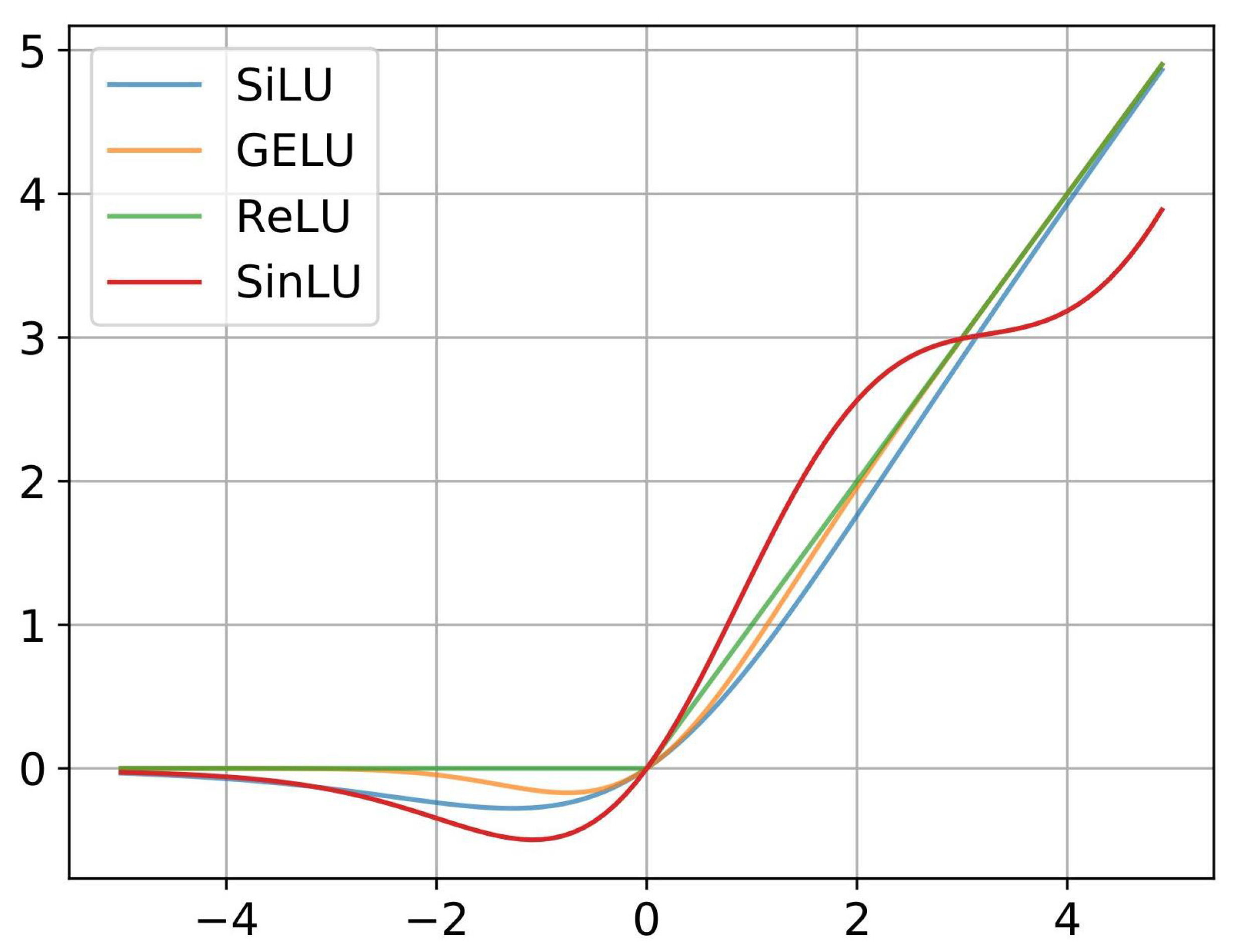
Keeping the above facts in mind, in this paper, we propose a new non-linear trainable activation function, called Sinu-sigmoidal Linear Unit (SinLU). Here, we explored the sinusoidal properties in an activation function while maintaining a ReLU-like structure. SinLU is a continuous function with a buffer zone on the negative side of the x-axis similar to GELU and SiLU. Furthermore, SinLU is trainable, which means it includes some parameters that get trained during the model training, which alters its shape. We demonstrated its efficiency and robustness, and found that any deep learning model with this novel activation function outperforms the models with other popular activation functions across domains, such as image classification and sequential data classification.

The paper is structured as follows: Section 2 provides a quick review of the past methods related to the research topic under consideration. In Section 3, we discuss the proposed approach. Section 4 presents the results followed by a brief discussion. We end with concluding remarks, outlining some future research plans in Section 5.

2. Related Work

Several developments pertaining to activation functions can be found in the literature from the past decade. One of the key features of an activation function is its non-linearity, which allows the NNs to be built deep. This non-linearity of the functions has also been claimed by the authors in [10,11], where it was also shown that activation functions should be non-constant and bounded. Moreover, the functions should be continuous and monotonically increase for the network to maintain its universal approximation property. An activation function is defined as a function $f:\mathbb{R}⟶\mathbb{R}$ as reported in [12]. Thus, the definition states that an activation function is a mapping from a subset of real numbers to a subset of real numbers, given that the network’s universal approximation property is not violated.

Studies point to the fact that bounded activation functions (such as identity function, step function, bipolar function, sigmoid function) yield impressive results, but only where the architecture of the is NN used shallow [13,14]. When deep networks are trained using such activation functions, unfortunately, the networks fail to learn due to the vanishing gradient problems [15]. In [16,17], it was shown that networks that use unbounded, non-polynomial activation functions (such as ReLU [3]) act as universal approximators. Such functions also help to lessen the vanishing gradient problems that are prevalent among the bounded activation functions, such as sigmoid function and identity function.

Myriad activation functions have been proposed throughout the years, many of which have been motivated by ReLU [13] and, hence, they bear resemblance to it. Some minor changes have been introduced into the variants with respect to ReLU. The original ReLU function was defined as $ReLU\left(x\right)=max(0,x)$. Apart from dealing with the vanishing gradient problem, it also enhances sparse coding [18,19], which ensures that the percentage of neurons that are active at any particular instant of time is usually less than 50%. However, one drawback of this activation function is the dying ReLU problem [20], which is the non-differentiability of the function at $x=0$. One of the first such activation functions that is based on the original ReLU function is leaky ReLU (LReLU) [20]. The LReLU activation function introduces a small gradient to the function when the unit is not active and saturated (when $x\le 0$, x being the independent variable). However, it does not improve the performance of the network significantly and it has been seen to exhibit a performance that is nearly identical to the standard rectifiers. A randomized version of it, called randomized Leaky ReLU, was proposed in [21], where the weight value for x, the independent variable, was sampled by a uniform distribution $\mathcal{U}(l,u)$ where, $0\le l<u<1$.

Another variant of ReLU is Sigmoid-weighted Linear Unit (SiLU), as proposed by the Elfwing et al. [22]. It is a sigmoid function that is weighted by the input, $SiLU\left(x\right)=x\sigma \left(x\right)$, where $\sigma$ denotes the sigmoid function. Moreover, the authors proposed the derivative of this SiLU as an activation function; $dSiLU\left(x\right)=\sigma \left(x\right)(1+x(1-\sigma \left(x\right)\left)\right)$. These functions yield very good results on reinforcement learning tasks.

Hendrycks et al. [8] proposed the GELU, which is another activation function that enhances the performance of the neural network. The definition of the GELU activation function is given by $GELU\left(x\right)=x\varphi \left(x\right)$, where $\varphi$ denotes the standard Gaussian cumulative distribution function. An empirical evaluation of the GELU function was done by the authors against the RELU and other activation functions, and the enhancement in performance was clearly demonstrated in a myriad of domains; thus, making it a viable alternative to the previous nonlinearities.

Kiselak et al. [23] proposed the scaled polynomial constant unit activation function (SPOCU) and it has been shown to yield satisfactory results on a wide range of problems. The authors also illustrated that SPOCU exceeds the performance of the existing activation functions, such as ReLU, on generic problems. One of the interesting properties of this activation function is its genuine normalization of the output layers. It has been tested on various datasets, and the results are compared with ReLU and scaled exponential linear unit (SELU) activation functions.

In a recent study by Liu et al. [24], the authors proposed the Tanh exponential activation function (TanhExp), which improves the performance of lightweight or mobile neural networks used for real-time computer vision tasks, and contains fewer parameters than usual. It enhances the performance of these networks on image classification. TanhExp is defined as $f\left(x\right)=xtanh\left(e^x\right)$ . It has a lower bound approximately equal to −0.3532 and there is no upper bound (unbounded above). TanhExp has been shown to outperform the other activation functions in terms of both convergence speed and accuracy for image classification with lightweight networks.

In [25], the authors proposed the average biased ReLU (AB-ReLU). Popular CNNs, such as AlexNet and VGGNet, have been used as discriminative feature descriptors in computer vision. It was found that the ReLU discards some information, so as to introduce non-linearity. Using the AB-ReLU function at the last few layers enhances the discriminative ability of deep image representation with the trained model. It does so by exploiting some discriminative information not considered by the ReLU and, discarding the irrelevant information used by ReLU. When this approach was tested over various unconstrained and robust face datasets, such as labeled faces in the wild (LFW) [26] and PubFig [27], among others, the performance of AB-ReLU is quite better than that of ReLU. Liu et al. [28] proposed a new methodology to tackle the vanishing as well as the exploding gradient problems, and the saddle point issue by operating the gradient activation function on the gradient. This function limits the higher values of the gradients and magnifies very small values of the gradients. Wang et al. [6] proposed a new activation function, called rectified linear Tanh, which ameliorates the performance of the Tanh function. It helps mitigate the vanishing gradient issue by using a linear function to replace the saturated regions of Tanh. Nag et al. [29] proposed an activation function, called Serf, which is non-monotonic as well as self-regularized, and it addresses issues, such as the Dying ReLU problem. Zhu et al. [30] proposed an activation function, named Logish, which is non-monotonic in nature. A logarithmic operation was performed to lessen the range of the sigmoid function and a variable was employed to introduce a strong regularization effect into the output. Maniatopoulos et al. [31] proposed an activation function incorporating a myriad of features from several activation functions of the ReLU family that give good performances, and it introduces a learnable parameter to adapt better to the data.

3. Proposed Approach

In this section, we discuss the proposed activation function Sinu-sigmoidal Linear Unit (or SinLU), which is defined by Equation (1).

$$SinLU\left(x\right)=(x+asinbx)·\sigma \left(x\right)$$

(1)

Here $\sigma$ is a sigmoid function and a and b are the trainable parameters.

$$\sigma \left(x\right)=\frac{1}{1+e^{-x}}$$

(2)

3.1. Formulation of SinLU

The proposed activation function is inspired by the properties of trainable parameters, sinusoid and ReLU-like activation functions. In the ReLU activation function, the output of a neuron is multiplied by 1 or 0. This hard gating property often leads to some minor information loss. Introducing the cumulative distribution function (CDF) of the standard normal distribution to the ReLU helps in smoothing the output near $x=0$. The CDF of the logistic distribution, $\sigma \left(x\right)$ can also be used, and it is known as SiLU $x·\sigma \left(x\right)$. We introduce sinusoidal periodicity at this stage. Multiplying $\sigma \left(x\right)$ with $x+sinx$ instead of x adds a wiggle in SiLU, resulting in a modified loss landscape. We define this function as $SinL{U}_{basic}$, which is formulated in Equation (3).

$$SinL{U}_{basic}=(x+sinx)·\sigma \left(x\right)$$

(3)

A more useful shape of the activation function can be devised by the introduction of some trainable parameters. We propose two such parameters, a and b, as shown in Equation (1). The parameter a denotes the amplitude of the sine function, which basically determines the participation of the sinusoid in the activation function. A very high value of a may lead to a shape that is nowhere close to a ReLU-like function. The parameter b determines the frequency of the sine wave. Figure 1 gives an idea about how the parameters shape the SinLU curve. This can be very easily avoided by proper initialization and hyperparameter-controlled training. We start with value 1 for both a and b and train these parameters with the same learning rate as used for the rest of the network.

3.2. Properties of SinLU

SinLU maintains a sparsity of its outputs, which means, for a randomly initialized network, not all of the neurons will be activated. As x tends to negative infinity, $SinLU\left(x\right)$ approaches 0, which ensures the sparsity. Figure 2 shows that SinLU has a buffer region left to the origin similar to GELU and SinLU. In this region, the minima of SinLU resides. The function $SinL{U}_{basic}$ reaches its minimum value near $x=-1.083$ and the value is approximately $-0.497$. With the trainable parameters of SinLU, this buffer zone is modifiable. The value of a is proportional to the magnitude of the minimum value. If the value of b is increased, the minimum value point moves closer to the y-axis. The steeper gradient near x is 0.

The recent activation functions based on ReLU attempt to modify the negative part of the ReLU, keeping the positive part intact. However, in our work, the sine function has its effect mainly in the positive part of the function. We also modify the self-gated properties, which is followed by GELU and SiLU. The self-gated property refers to functions having the form $f\left(x\right)=xg\left(x\right)$ but the proposed function has the form of $f\left(x\right)=(x+h(x\left)\right)g\left(x\right)$. These non-conventional properties allow the proposed activation function to act differently than the ReLU-family and pave the path for some future functions that follow these properties.

4. Experimental Results and Discussion

In this section, we performed multitudes of experiments to test the effectiveness of the proposed activation function. We compare the performance of the proposed SinLU against ReLU, GELU, and SiLU. These specific functions were chosen based on their heavy usage and similarity in shape with the proposed function. The experiments were performed on some standard datasets and multiple types of models were used.

4.1. MNIST

The MNIST dataset is an image classification dataset for handwritten digit classification. It contains 60,000 train images and 10,000 test images belonging to a total of 10 classes. A number of experiments were performed on this dataset to show how the proposed activation function, SinLU, works in comparison to other similar activation functions.

4.1.1. Lightweight Neural Networks

We used different NN based architectures to experiment with the proposed activation function. For the first set of experiments, we used NNs with no convolution. The experiments were conducted for single layer feed-forward networks (SLFN) as well as deeper networks with more than one layer. The values of the hyperparameters used in these experiments are mentioned in

Table 1. Hyperparameters used for the experiments with SLFN, DNN, and CNN models.

Hyperparameter	Value
Learning rate	$3\times {10}^{-4}$
Batch size	32
Number of epochs	10
Scheduler step	2

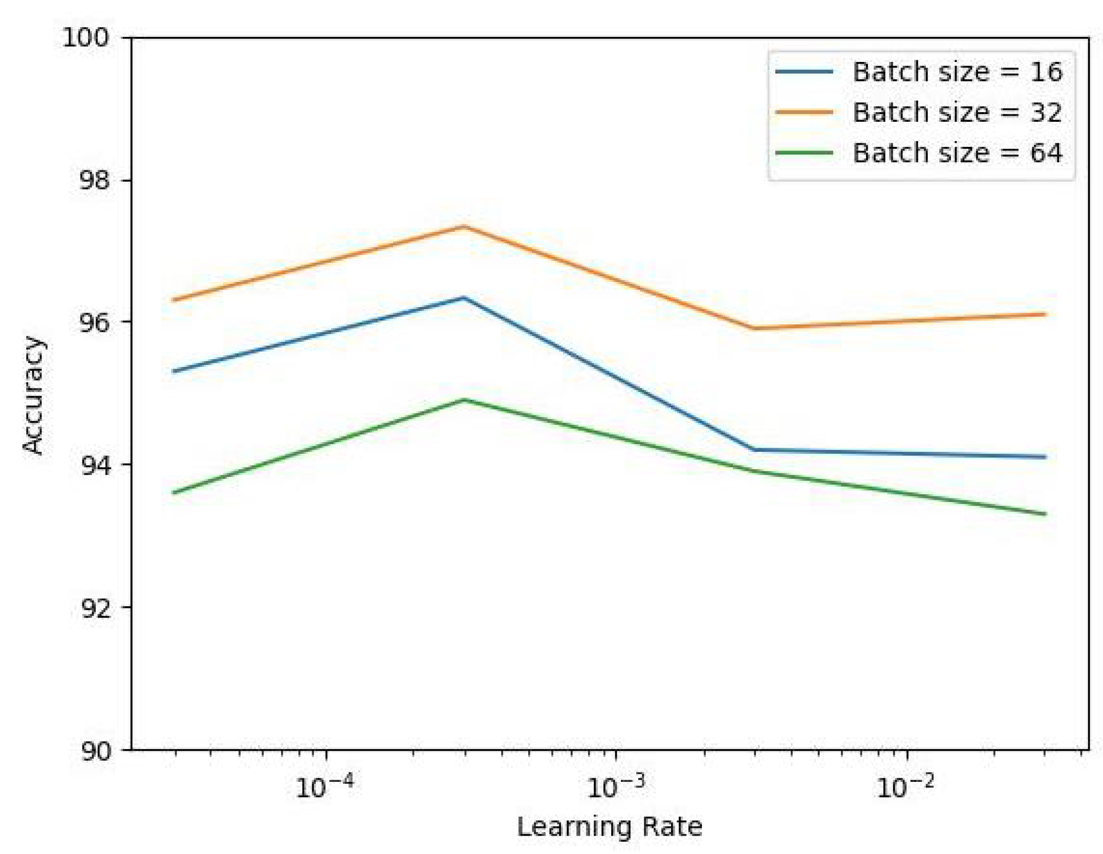
. For the hyperparameter optimization, grid search method was used. Figure 3 shows the accuracy on the MNIST dataset with a SLFN utilizing SinLU. It can be observed that, for higher and lower values of the learning rate, as well as batch size, we obtained a lower accuracy value. For the training, we used the Adam optimizer and the learning rate decreased after every two steps by an exponential learning rate scheduler. This particular setup was also used for the experiments in Section 4.1.2–Section 4.1.4.

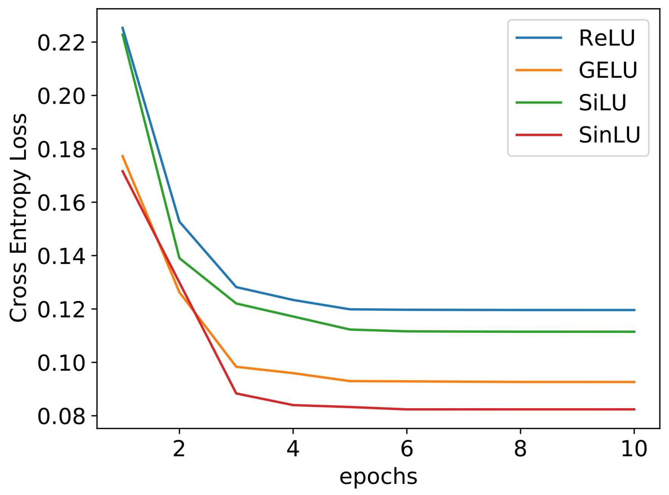
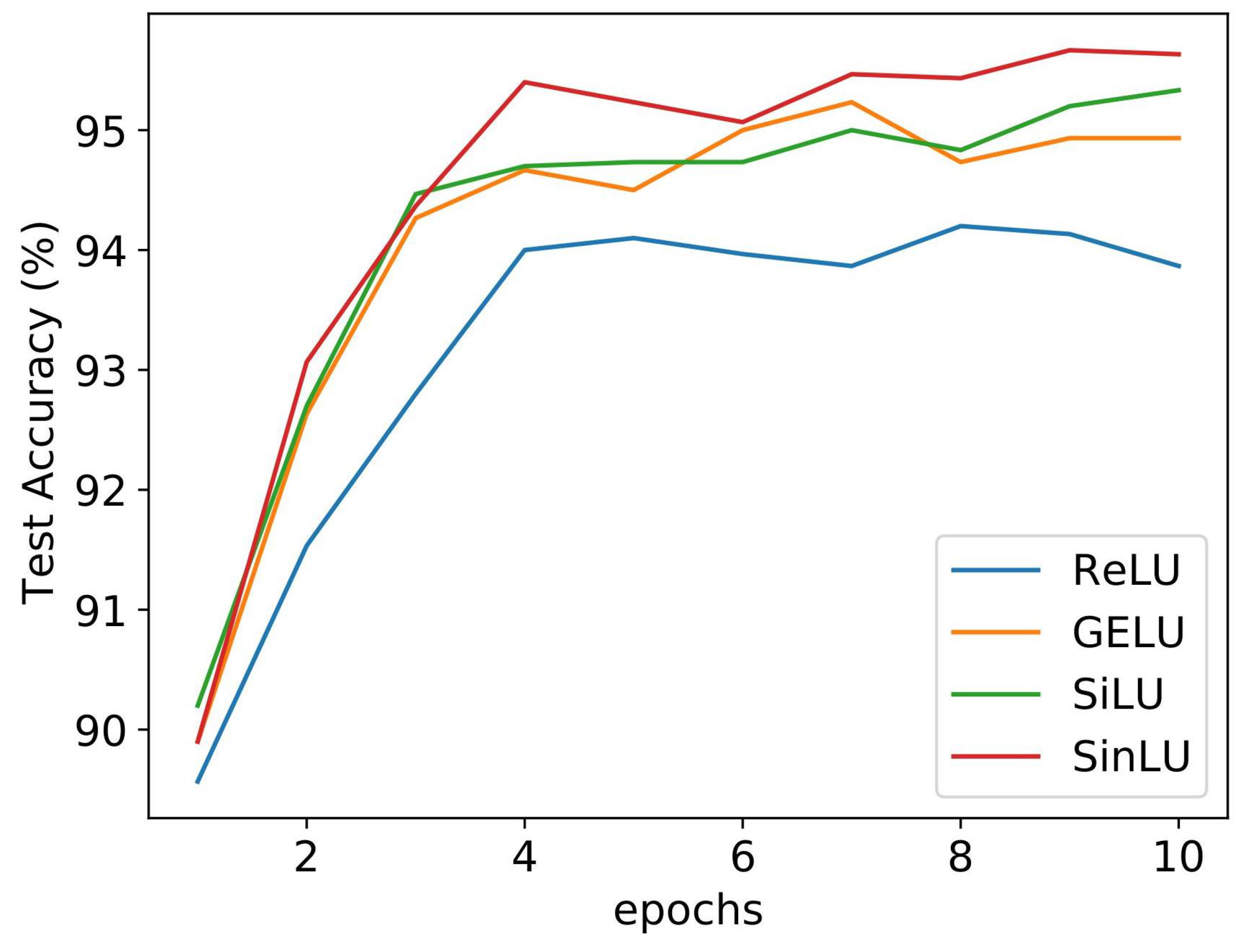
The SLFN consists of a hidden layer of size 512. Figure 4 shows the convergence graph for different activation functions. We compared the proposed SinLU activation function against ReLU, GELU, and SiLU activation functions. The SLFN utilizing SinLU gave us a training accuracy of 97.33% and test accuracy of 97.11%. Figure 4 shows the convergence of the networks with different activation functions. It can be clearly observed that, in the case of lightweight neural networks, such as SLFN, SinLU converges faster than the other activation functions.

Table 2. Training and test accuracies on the MNIST dataset with SLFN.

Activation Function	Training Acc. (%)	Test Acc. (%)
ReLU	96.13	95.79
GELU	97.20	96.67
SiLU	96.12	95.75
SinLU	97.33	97.11

can be referred to for an understanding of how the proposed activation function works in terms of accuracy, in comparison with other activation functions.

4.1.2. Performance over Noise

To show the robustness of the proposed activation function, we conducted experiments involving multiplicative Gaussian noise at each layer, which is also known as Gaussian dropout. The idea of the dropout is to multiply hidden activation with random variables that follow the normal distribution. Equation (4) shows the relationship between the standard deviation of the Gaussian distribution and dropout rate. For these experiments, the value of the dropout rate was taken as 0.25.

$$Stddev=\frac{rate}{1-rate}$$

(4)

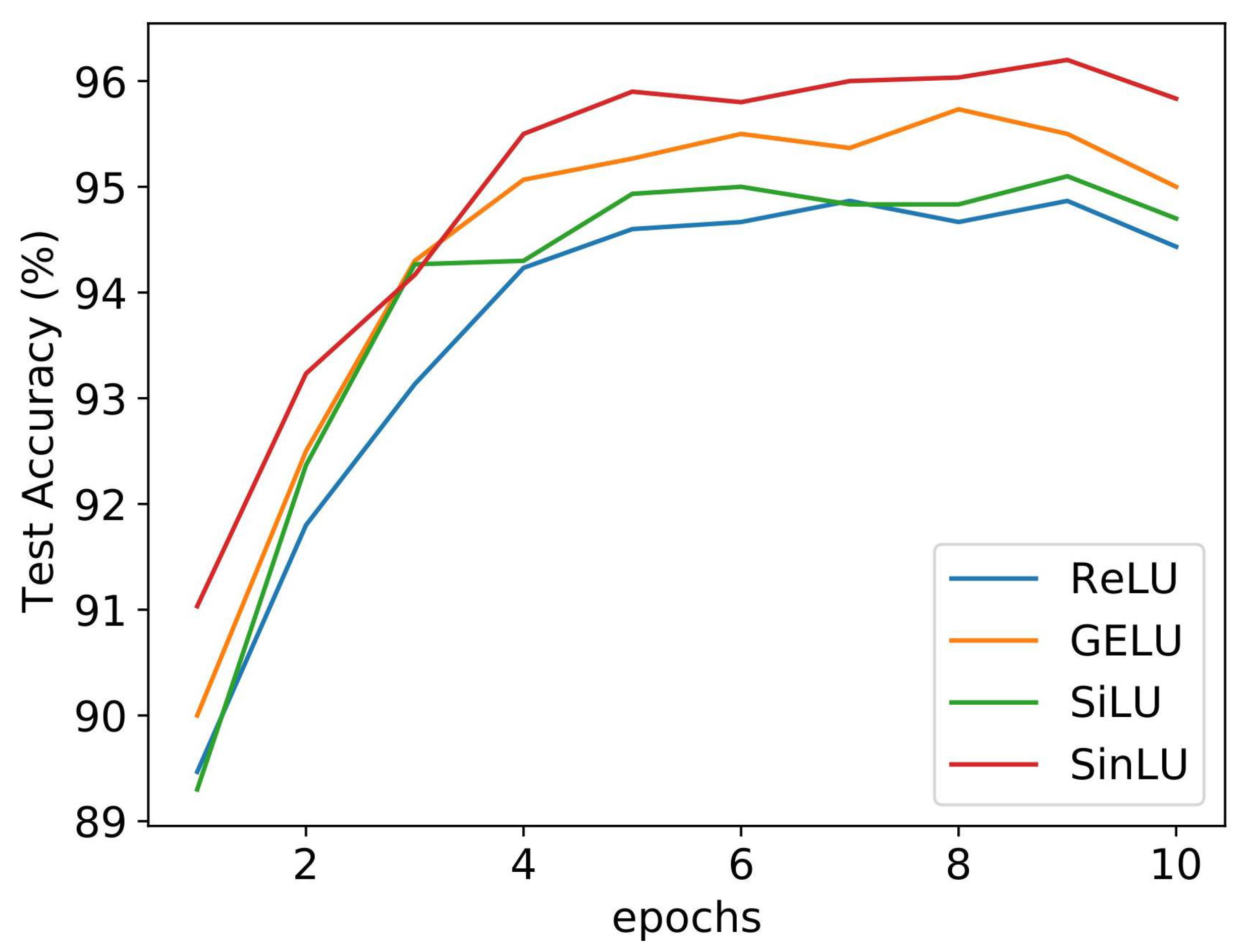
Two lightweight NN architectures were chosen for this set of experiments. One was the SLFN, as described above, and the other was an NN with two hidden layers. Let us call this deeper network DNN. The hidden layers of this DNN are also of size 512. Gaussian dropout was implemented after all of the hidden layers for both SLFN and DNN. Figure 5 and Figure 6 show the performances of different activation functions on SLFN and DNN, respectively. For both networks, it can be observed that SinLU was the least affected by the introduction of the Gaussian noise. Activation functions, such as ReLU, performed very poorly in SLFN. Although other activation functions improved their performances by small amounts in the DNN, we can observe that SinLU outperformed all other activation functions.

We also measured the performances of the said activation functions with salt and pepper noise. This noise was applied to all of the layers with a probability of 0.05 (the probability that a data point in the output tensor of a layer would be affected by noise was 0.05) and with a salt to pepper ratio of 0.5. Experimentation was conducted for both SLFN and DNN, as defined above.

Table 3. Test accuracy achieved by different activation functions on SLFN and DNN networks with introduction to salt and pepper noise.

Activation Function	SLFN Acc. (%)	DNN Acc. (%)
ReLU	94.47	94.09
GELU	95.57	95.83
SiLU	95.33	94.95
SinLU	96.47	95.83

shows the test accuracy achieved by the models for different activation functions. It can be easily observed that, in this case, SinLU outperformed other activation functions.

4.1.3. Deeper Models Overfitting

Adding more layers to an NN often results in better learning, as more information is retained in a larger number of neurons. However, with deeper networks, the risk of overfitting increases. With a very large number of layers, the model learns the training data too well and is unable to perform on unseen data.

We performed the experiment to show how SinLU performs with an increasing number of layers in an NN. The size of all of the hidden layers was 512. Figure 7 shows the test accuracy on the MNIST dataset for NN models with the increasing number of hidden layers. It can be observed that the models utilizing ReLU and GELU began to overfit heavily as soon as the number of hidden layers reached 15. All of the activation functions, except SinLU, performed poorly with models getting deeper. It can be observed that, even if the NN model got deeper, the proposed activation function performed almost the same. There was not even a small amount of reduction in test accuracy for SinLU as the number hidden layers became 20. It is very likely that this high resistance to overfitting comes from the better gradient flow of SinLU during backpropagation. It was already mentioned that the shape of SinLU helps in overcoming the gradient-related problems, such as vanishing gradient, and dying ReLU problems, and this property helps the parameters of the deeper NNs to learn better.

4.1.4. CNN on MNIST-like Datasets

All experiments up to this subsection were performed with only vanilla NNs, having only fully connected layers (no convolutions). We used CNNs with the proposed activation function to classify the images of the MNIST dataset. We also tested on datasets similar to MNIST to gain a better understanding of the performance of the proposed activation function.

The CNN consisted of seven convolution layers and two maxpool layers. Each convolution layer was followed by batch normalization and the activation function under observation. The feature map obtained from the final convolution layer was of dimension $256\times 7\times 7$. An adaptive average pooling was performed with output size $2\times 2$ and flattening was done, resulting in a 1024 dimensional vector. This further passed through a fully connected network with a hidden layer size of 512.

The QMNIST dataset is just an extension to the MNIST dataset, with 50,000 more generated images. Fashion MNIST is a image classification dataset consisting of clothing items. The images of this dataset belong to 10 different classes, which are T-shirt, shirt, pullover, dress, coat, trouser, sandal, sneaker, bag, and ankle boot. The KMNIST or Kuzushiji-MNIST dataset is an image classification dataset of 10 Hiragana characters used in the Japanese writing system. All four datasets contain gray scale images of sizes $28\times 28$ and no further resize operations have been done before the experiments. Though fashion MNIST and KMNIST have the same dataset sizes as MNIST, the complexity and diverse distributions of images make the task more difficult than MNIST.

Table 4. Test accuracy (in %) obtained by CNN with different activation functions on various datasets. Bold value suggests the best accuracy score in the row.

Dataset	ReLU	GELU	SiLU	SinLU
MNIST	99.5	99.52	99.4	99.6
Fashion-MNIST	92.57	92.75	92.66	93.5
KMNIST	97.87	97.42	97.82	98.05
QMNIST	99.43	99.52	99.44	99.49

shows the test accuracy obtained in the mentioned datasets with CNN utilizing different activation functions. As CNNs are very effective models when it comes to image classification, the test accuracies obtained in MNIST and QMNIST are very high, irrespective of the activation functions. Though SinLU produces the best accuracy score on MNIST, with the dataset QMNIST, GELU outperforms SinLU, but by a small margin. In the case of fashion MNIST and KMNIST, as the classification task is difficult, we observe that SinLU outperforms other activation functions by a larger margin. This proves the robustness of the proposed activation function over different datasets.

4.2. CIFAR

We further investigated the ability of the proposed activation function in the domain of image classification with more difficult datasets. In this set of experiments, we used both CIFAR-10 and CIFAR-100 datasets. CIFAR-10 is a 10-class image dataset, where each class has 5000 training images and 1000 test images. CIFAR-100 is a 100-class dataset where each class has 500 training images and 100 test images, making it a more complex dataset. Images in CIFAR-10 and CIFAR-100 datasets are $32\times 32$ three-channel (RGB) images.

4.2.1. Transfer Learning

In this set of experiments, we used transfer learning to create the classification models. In transfer learning, weights from pre-trained models (which are generally trained on bigger datasets, such as the ImageNet dataset) were fine-tuned on a target dataset to achieve the desired classifier model. The pre-trained models used in this set of experiments were MobileNetV2, ResNet50, VGG16, AlexNet, and ShuffleNet, with their activation functions replaced as required.

Table 5. Test accuracy (in %) obtained by transfer learning models with different activation functions on CIFAR10. Bold value suggests the best accuracy score in the row.

Model	ReLU	GELU	SiLU	SinLU
MobileNetV2	81.4	81.31	79.71	81.55
VGG16	88.84	89.77	89.87	89.91
ResNet50	83.08	82.76	80.23	83.6
AlexNet	91.94	91.88	91.48	91.34
ShuffleNet	75.02	77.51	76.71	77.71

shows the accuracy achieved by various transfer learning models with different activation functions on the CIFAR-10 dataset. We can observe that the proposed SinLU activation function produced the best results for all of the pre-trained models except for AlexNet. If we discard SinLU, it can be observed that no single activation function performs the best for all of the models. In that aspect, we can infer that SinLU performs better than the other activation functions overall.

Table 6. Test accuracy (in %) obtained by transfer learning models with different activation functions on CIFAR100. Bold value suggests the best accuracy score in the row.

Model	ReLU	GELU	SiLU	SinLU
MobileNetV2	54.04	54.73	51.61	54.73
VGG16	62.59	63.31	63.28	60.84
ResNet50	60.75	56.88	52.49	60.05
AlexNet	51.32	50.37	51.41	51.77
ShuffleNet	43.61	46.37	46.94	48.80

shows the similar result for CIFAR-100 dataset. Here, we can observe that for MobileNetV2, AlexNet, and ShuffleNet, the proposed SinLU produces the best results. Even for ResNet, the accuracy score is 0.7% less than the best accuracy.

4.2.2. With Gradient Activation Function

While training deep neural networks with a backpropagation algorithm, the gradient flows through the layers of the network. A gradient activation function (GAF) [28] improves upon the tiny and large gradients, resulting in a better gradient flow. For this set of experiments, we used a CNN consisting of three blocks where each block was made up of two convolution layers and a maxpool layer. For the first block, the convolution layers had 32 and 64 output channels, respectively. For the second block, both of the Conv layers had an output depth of 128; for the third block, it was 256. The feature maps of dimensions 25,644, obtained from the final block, were flattened before passing through the FC layer. This network was trained with SGD and Adam optimizer with a learning rate of $3\times {10}^{-4}$ for 10 epochs. GAF was utilized for both of these optimizers and the arctan GAF function was used. The hyperparameters for arctan GAF were taken as $\alpha =0.1$ and $\beta =20$. The test accuracy obtained on each of the trained models is shown in

Table 7. Test accuracy (in %) obtained by CNN with different activation functions on the CIFAR10 dataset for two different optimizers, SGD and Adam with arctan GAF [28]. The bold value suggests the best accuracy score in the row.

Activation Function	SGD Arctan	Adam Arctan
ReLU	47.1200	81.9867
GELU	39.2667	81.8667
SiLU	33.9600	81.8933
SinLU	68.7867	81.9867

. From the results, it can easily be seen that SinLU produces the best accuracy among other activation functions. The GAF helps the network to converge faster, and if we observe the results with SGD, it can be seen that the network with SinLU converges much faster than the other networks. Though for Adam, all networks perform very similar, the network with SinLU achieves the highest accuracy along with ReLU.

4.3. Sequential Data

From the UCI machine learning repository, the heterogeneity human activity recognition (HHAR) [32] dataset was used to test the efficiency of the new activation function proposed here, while being deployed by recurrent neural networks (RNNs). Recorded from smartphones and smartwatches, the HHAR dataset was designed to portray the noticeable heterogeneities in real-time implementations. Myriad device models and use-scenarios have aided in constituting the dataset. The dataset was used to yardstick human activity recognition algorithms. . The activities involve: ‘biking’, ‘sitting’, ‘standing’, ‘walking’, ‘stair up’ and ‘stair down’; hence, there are six output classes.

Of the 10,299 examples present, 7352 were used for training the models and the rest, 2947, were used to test on the dataset.

Long short-term memory (LSTM) networks are a sort of RNN—a competent of learning and doing well-gauged predictions in models of sequence prediction. LSTMs are of great help in modeling univariate time series forecasting problems, which are generally made of a set of observations; we designed the prototype or model to learn from the past set of readings to forecast the next value that will follow this sequence of readings. We used five different LSTM models to conduct the predictions on the UCI HHAR dataset. They are: vanilla LSTM [33], stacked LSTM [34], bidirectional LSTM [35], residual LSTM [36], and bidirectional residual LSTM [37]. In LSTM, the network runs the input from the past to the future, while, in the bidirectional ones, it runs the input in two ways. The first way is from the past to the future and the second way is from the future to the past, thus preserving information from both the past as well as the future. The vanilla LSTM model comprises a single hidden layer of LSTM, along with an output layer that is used to make a prediction. The stacked LSTM model consists of multiple hidden LSTM layers that are stacked on top of each other. In residual LSTM, there is a spatial shortcut path from the lower layers that augment the efficiency while training of the deep networks that comprise a myriad of LSTM layers. This functionality is not present in the other LSTM models mentioned earlier. The third model incorporates the traits of both these models and, thus, delivers better performance among the three.

The values of the hyperparameters that were obtained after the LSTM network were trained and are recorded in

Table 8. Hyperparameters used to train the LSTM network.

Attribute	Value
batch_size	64
num_epochs	120
drop_probabililty	0.5
num_epochs_hold	100
num_layers	2
learning rate	0.0015
weight_decay	0.001

. The number of classes is 6. The number of hidden layers is set to 32 for each of the models, except the vanilla LSTM model that has a single hidden LSTM layer. The number of residual layers is 2 and the number of highway layers is 2 for the residual LSTM model and the bidirectional residual LSTM model. The number of highway layers is 1 in the bidirectional LSTM model.

In

Table 9. Testing accuracy obtained on the UCI HHAR dataset when various models were trained using different activation functions. The bold value suggests the best accuracy score in the column.

Act Fn	Vanilla LSTM	Stacked LSTM	Bidir LSTM	Res LSTM	BidirRes LSTM
SinLU	0.7035	0.8534	0.8747	0.8879	0.8979
ReLU	0.7024	0.8621	0.8734	0.8965	0.8802
GELU	0.7034	0.8439	0.8761	0.8493	0.8602
SiLU	0.7025	0.8386	0.8961	0.7085	0.8935

, the test accuracy of each of the activation functions was tabulated for the three different LSTMs that were chosen. It is clearly evident that the SinLU activation function works as well as any of the others. In the bidirectional residual LSTM model, as well as the vanilla LSTM model, it gives us the best performance, while in the other two, its performance does not lag behind the best one by a huge margin. Its good performance is also held up in

Table 10. Testing loss observed on the UCI HHAR dataset when various models were trained using different activation functions. The bold value suggests the least testing loss in the column.

Act Fn	Vanilla LSTM	Stacked LSTM	Bidir LSTM	Res LSTM	BidirRes LSTM
SinLU	1.3212	1.1923	1.1689	1.1573	1.1457
ReLU	1.3341	1.1808	1.1705	1.1468	1.1632
GELU	1.3233	1.2212	1.1671	1.1944	1.1835
SiLU	1.3489	1.2451	1.1471	1.3213	1.1501

and

Table 11. F1-Score obtained on the UCI HHAR dataset when various models were trained using different activation functions. The bold value suggests the best F1-score in the column.

Act Fn	Vanilla LSTM	Stacked LSTM	Bidir LSTM	Res LSTM	BidirRes LSTM
SinLU	0.6998	0.8512	0.8745	0.8878	0.8975
ReLU	0.6825	0.8618	0.8751	0.8973	0.8797
GELU	0.6963	0.8444	0.8752	0.8512	0.8604
SiLU	0.6861	0.8372	0.8964	0.6454	0.8944

. The former table shows the model loss on the test set and the latter shows the F1 score achieved. The results obtained from SinLU are superior if we look at the good performances delivered by it in the bidirectional residual LSTM model and the vanilla LSTM model. Moreover, the results obtained if the SinLU were used as the activation function in the bidirectional LSTM model; the residual LSTM model and the stacked LSTM model were comparable to the other activation functions. The accuracy and F1-score are towards the higher side and the loss is towards the lower side, as expected.

5. Conclusions

In this work, we proposed a novel activation function, which is named as SinLU. The addition of the sinusoidal periodicity into the sigmoidal linear unit aids in preventing the information loss and, thus, a better loss landscape. To define a proper shape of the activation function, we used two parameters, which are trainable. The defined activation function proves its competence by delivering results that are comparable to the other standard activation functions, and in a myriad of occasions, outperforms them. One of the limitations of the proposed activation function involves the computational complexity. The calculation of the activation using the Equation (1), as well as its gradient, will take a slightly longer time than other ReLU-like functions.

The proposed activation function is yet to be tested on other domains, such as reinforcement learning; hence, future work can focus on this. Moreover, we can also test how the function performs on transformer-based models, such as GPT-3, vision transformer, etc.

The source code of this present work is available at LINK.