Modeling and Numerical Simulation of the Thermal Interaction between Vegetation Cover and Soil

Abstract

In this work, we propose a mathematical model representing the thermal interaction between vegetation cover and the soil underneath it. This model consists of a one-dimensional reaction–diffusion equation describing the evolution of the temperature in the vegetation cover coupled with a two-dimensional reaction–diffusion equation to represent the evolution of the temperature in the soil. The thermal interaction between the vegetation cover and the soil is studied and the distribution of temperatures in the soil with depth is also obtained. The vegetation cover acts in this model as a dynamic and diffusive boundary condition for the soil. The developed model takes into account the latent heat of fusion, which appears when the transformation of ice into liquid water or vice versa occurs inside the soil. The numerical approach for the solution of the mathematical model conducted in this work is based on the finite volume method with Weighted Essentially Non-Oscillatory technique for spatial reconstruction and the third-order Runge–Kutta Total Variation Diminishing numerical scheme is used for time integration, which is very efficient to obtain the numerical solution of this type of model. Some numerical examples are solved to obtain the distribution of temperature both in the vegetation cover and the soil.

1. Introduction

This work deals with the introduction of a mathematical model aimed at describing the thermal interaction between vegetation and soil. The main feature of this model is how the temperature inside the ground is affected by the vegetation on the surface. Several aspects of the vegetation are considered in the model, such as the Leaf Area Index (LAI), the latent heat of vaporization, the sensible heat flux, the density of the foliage, or emissivities, just to name a few of them. Some of these characteristics are typically used to study vegetation–soil interaction in green roof modeling, such as in [1,2]. Background on different aspects of the evolution of temperature in soils can be found—for instance, in [3], where the determination of the evolution of temperature with depth is used for geothermal energy applications. Soil temperature is also important in seed germination and plant growth (see for instance [4]), for which the determination of the temperature in the region of the ground close to the surface is of great importance, since this is the region where the most important thermal phenomena take place. In [5], the prediction of ground temperature variation with depth for Jamshedpur (India) for different values of air temperature and solar radiation was studied, based on a finite difference scheme. As referred to in [6] and the references therein, there is a strong dependence of soil temperature with surface cover, which also affects the fraction of solar radiation reflected by the surface—that is, the albedo. Both concepts, albedo and coalbedo, are very relevant in models accounting for thermal interaction between vegetation and soil. Coalbedo, which is equal to 1-$albedo$, is the fraction of the radiation that is absorbed by the surface, which has an effect on soil temperature.

The model studied in this work is built on a two-dimensional domain, where x represents the horizontal coordinate and z stands for the ground depth. The vegetation layer is considered to be located at the upper edge of the domain; hence, it is assumed to be one-dimensional and acts as a dynamic and diffusive boundary condition to obtain the evolution of the temperature in the ground. The numerical resolution is performed by means of a finite volume (FV) scheme with Weighted Essentially (WENO) reconstruction in space and a third order Runge–Kutta TVD (RK3-TVD) scheme for time discretization. The rest of the document is organized as follows. In Section 2, we describe the mathematical model introduced to represent the vegetation cover and its interaction with soil. Section 3 is devoted to a brief description of the numerical method used. In Section 4, numerical examples are given. Section 5 presents the conclusions and discussion.

2. The Model

We consider a rectangular $2D$ domain, where the upper boundary represents the $1D$ vegetation cover. In Figure 1, a sketch of the $2D$ domain is shown. The region of the soil where the main interaction processes between the soil and the vegetation cover take place is the top soil and, hence, this is the zone where the most important variations in temperature occur, as will be verified in the numerical simulations.

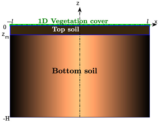
Figure 1. The spatial domain considered in this model is a rectangle, whose upper edge is the $1D$ vegetation cover. The region denoted as top soil, $(x,z)\in [-l,l]\times [z_m,0],$ is the part of the ground that is thermally influenced by the vegetation cover.

The equation representing the evolution of the temperature in the vegetation cover is given as

$$C_v\frac{\partial T_v}{\partial t}-\frac{\partial }{\partial x}\left(K_{H0}\frac{\partial T_v}{\partial x}\right)+K_V\frac{\partial T_s}{\partial n}=F_v,$$

(1)

where $T_v=T_v(x,t)$ is the temperature of the vegetation cover, $T_s=T_s(x,z,t)$ is the temperature of the soil, $K_{H0}$ is the heat conductivity of the vegetation cover, $K_V$ is the conductivity of the soil in vertical direction, $C_v$ represents the heat capacity of the vegetation cover, x is the spatial coordinate, and t is time. The term $K_V\frac{\partial T_s}{\partial n}$, which includes the normal derivative of the soil temperature, represents the influence of soil temperature on the upper boundary where the vegetation is located. This term has been introduced to account for conduction phenomena from the ground to the vegetation cover.

In (1), the source term is given by

$$F_v={\sigma }_v\left(R_{av}+{ϵ}_v{I}_{ir}-{ϵ}_v\sigma T_v^4\right)+\frac{{\sigma }_v{ϵ}_s{ϵ}_v\sigma }{{ϵ}_l}(T_s^4-T_v^4)+H_v+L_v,$$

(2)

where $H_v$ represents the sensible heat flux, which stands for the energy loss due to heat transfer from the vegetation cover to the surrounding air. Its expression, following [7,8], is

$$H_v=(e_0+1.1LAI{\rho }_{af}{C}_a{C}_f{W}_{af})(T_a-T_v),$$

(3)

where $e_0$ is the windless exchange coefficient depending on temperature difference; $LAI$ is the leaf area index, which is a dimensionless quantity defined as the one-sided green leaf area per unit ground surface area. The density of the foliage is represented by ${\rho }_{af}$. $C_a$ is the specific heat of air at constant pressure; $C_f$ stands for the bulk transfer coefficient, given by the expression $C_f=0.01(1+0.3/W_{af})$, as proposed in [9], where $W_{af}$ is the wind speed at the interface of air–foliage. $T_a$ represents the ambient temperature, while $T_v$ is the temperature of the vegetation cover. In (2), the emissivities of the vegetation cover ${ϵ}_v$ and the soil ${ϵ}_s$ are also included. The emissivity represents the ability of a body to emit energy and ranges from 0 to 1. The parameter ${\sigma }_v$ represents the fractional vegetation cover, which is taken here as ${\sigma }_v=1-exp(-0.75LAI)$, as proposed in [10] for grasses. The absorbed solar radiation is taken in this work as $R_{av}=Q|cos\left(\frac{\pi t}{12}\right)-sin\left(\frac{\pi t}{12}\right)|{\beta }_v$, where Q is the solar constant and ${\beta }_v$ is the coalbedo (fraction of absorbed energy).

The latent heat flux is given by

$$L_v=LAI{\rho }_{af}{C}_f{l}_v{W}_{af}\tilde{r}(q_{av}-q_{fsat}),$$

(4)

where $l_v$ is the latent heat of vaporization, which, according to Henderson-Sellers [11], is given by

$$l_v=1.91846\times {10}^6{\left(\frac{T_v}{T_v-33.91}\right)}^{2}kJk{g}^{-1}.$$

(5)

In (4), the following coefficient was introduced

$$\tilde{r}=\frac{r_a}{r_a+r_s},$$

(6)

which represents the vegetation surface wetness factor, where the stomatal resistance is given by $r_s=\frac{r_{s,min}}{LAI}{f}_1{f}_2{f}_3$, where $r_{s,min}$ is the minimum stomatal resistance. The multiplying factor $f_1$ depends on solar radiation and, following [2], is given by

$$f_1=\left\{\begin{array}{ccc}-\frac{0.81(0.004I_s+1)}{0.004I_s+0.005}+\frac{0.81}{0.005},& if& I_s\le 1059.2\\ \frac{0.81}{0.005}& if& I_s>1059.2.\end{array}\right.$$

(7)

The factor $f_2$ depends on the moisture content. In the case of low moisture, the value considered is $f_2=\frac{100}{20}$, whereas for high moisture content, the value is $f_2=\frac{100}{70}$ (see [1,2] for details). Concerning the factor $f_3$, it is taken here as $f_3=1$. The resistance to moisture exchange offered by the boundary layer formed on the leaf surface, known as aerodynamic resistance, reads $r_a=\frac{1}{C_{fWaf}}$ (see [1]). The mixing ratio of the air within the vegetation layer (see [1,2]) is given by

$$q_{av}=\frac{(1-{\sigma }_v)q_a+{\sigma }_v(0.3q_a+0.6q_{f,sat}\tilde{r}+0.1q_{s,sat}{M}_g)}{1-{\sigma }_v(0.6(1-\tilde{r})+0.1(1-M_g))},$$

(8)

where $q_{s,sat}=\frac{0.622e_s}{Pa-e_s}$ is the saturated mixing ratio at the soil temperature and $q_{f,sat}=\frac{0.622e_v}{Pa-e_v}$ is the saturated mixing ratio at the vegetation temperature, with $e_s=\frac{e_{a0}exp\left(17.269(T_s-273.15)\right)}{T_s-35.86}$ being the saturated air vapor pressure at soil temperature and $e_v=\frac{e_{a0}exp\left(17.269(T_v-273.15)\right)}{T_v-35.86}$ representing the saturated air vapor pressure at vegetation temperature.

As for the equation for the evolution of the temperature in the soil, this is given by

$$\frac{\partial \gamma \left(T_s\right)}{\partial t}-\frac{\partial }{\partial x}\left(K_H\frac{\partial T_s}{\partial x}\right)-\frac{\partial }{\partial z}\left(K_V\frac{\partial T_s}{\partial z}\right)=F_s,$$

(9)

where $K_H$ and $K_V$ are the heat conductivities of the soil in x and z directions, respectively. Equation (9) considers the water phase change (ice–liquid water), which is represented by the function $\gamma \left(T_s\right)$. In this work, we use the following expression (see [8]),

$$\gamma \left(T_s\right)=\left\{\begin{array}{ccc}{k}_1{\tilde{T}}_s& if& T_s<273,\\ -(2L+\Delta k{ϵ}_0)\frac{{\tilde{T}}_s^3}{{ϵ}_0^3}+(3L+2\Delta k{ϵ}_0)\frac{{\tilde{T}}_s^2}{{ϵ}_0^2}+k_1{\tilde{T}}_s& if& 273\le T_s\le 273+{ϵ}_0,\\ L+k_2{\tilde{T}}_s& if& T_s>273+{ϵ}_0,\end{array}\right.$$

(10)

where ${\tilde{T}}_s=T_s-273$ and $\Delta k=k_2-k_1$.

In order to consider that the interaction between the vegetation cover and the soil takes place within the top soil, the right-hand side of Equation (9) is given by

$$F_s(x,z,t,T_s,T_v)=\left\{\begin{array}{ccc}{f}_{s,1}-f_{s,2}+H_s+L_s& if& z_m\le z\le 0\\ 0& otherwise,\end{array}\right.$$

(11)

where, as aforementioned, $z_m$ is the depth of the top soil, which is the zone of the soil where the influence of the vegetation takes place. In (9), $f_{s,1}$ and $f_{s,2}$ are defined by means of the Stefan–Boltzmann law for radiation and are expressed as

$$\begin{array}{c}{f}_{s,1}=(1-{\sigma }_v)(E-{ϵ}_s\sigma T{s}^4),\\ f_{s,2}=\frac{{\sigma }_v{ϵ}_v{ϵ}_s\sigma }{{ϵ}_l}(T_s^4-T_v^4).\end{array}$$

(12)

In expression (12), $E=R_{as}+{ϵ}_s{I}_{ir}$ is introduced, where $R_{as}$ is the radiation absorbed by the soil and is taken here as $R_{as}=Q\left|\right(sin\left(\frac{\pi t}{12}\right)+cos\left(\frac{\pi t}{12}\right)|{\beta }_s$, where ${\beta }_s$ is the coalbedo of the soil.

In (11), the following quantities are introduced

$$H_s=\left(e_0+{\rho }_{ag}{C}_a{C}_{hg}{W}_{af}\right)\left(T_a-T_s\right),$$

(13)

and

$$L_s=C_{eg}{l}_v{W}_{af}{\rho }_{ag}(q_{af}-q_g),$$

(14)

where $q_{af}=\frac{(1-{\sigma }_v)q_a+{\sigma }_v(0.3q_a+0.6q_{fsat}rseg+0.1q_{gsat}{M}_g)}{1-{\sigma }_v(0.6(1-rseg)+0.1(1-M_g))}$ with $rseg=\frac{r_a}{r_a+r_s}$, where $r_a=\frac{1}{C_f{W}_{af}}$ is the resistance to moisture exchange and $r_s$ is the stomatal resistance.

We also consider the Bulk Richardson number given by $R_{ib}=\frac{2g{Z}_a(T_{af}-Ts)}{(T_{af}+Ts)W_{af}^2}$. According to this value, the so-called atmospheric stability factor is defined as

$${\mathsf{\Gamma }}_h=\left\{\begin{array}{ccc}\frac{1}{\sqrt{1-16R_{ib}}}& if& R_{ib}<0\\ \frac{1}{1-5R_{ib}}& if& R_{ib}\ge 0.\end{array}\right.$$

(15)

In expression (13), the bulk transfer coefficient $C_{hg}$ can be expressed as a function of the bulk transfer coefficients near ground $C_{hnf}$ and close to the foliage–atmosphere interface $C_{hng}$, multiplied by the stability factor $G_h$ (see [1])—that is, $C_{hg}={\mathsf{\Gamma }}_h((1-{\sigma }_v)C_{hng}+{\sigma }_v{C}_{hnf})$ with $C_{hng}={\left(\frac{\kappa }{log(Z_a/z_{og})}\right)}^2$ and $C_{hnf}={\left(\frac{\kappa }{log(Z_a-Z_d/z_{of})}\right)}^2$, where $\kappa$ is the universal von Kármán constant, which is frequently used in turbulence modeling, as it happens in boundary-layer meteorology to account for fluxes of momentum, heat, and moisture from the atmosphere to the land surface. We also have the bulk transfer coefficient for latent heat exchange given by $C_{eg}={\mathsf{\Gamma }}_h((1-{\sigma }_v)C_{eng}+{\sigma }_v{C}_{hnf})$ and the mixing ratio at the ground surface $q_g=M_g{q}_{gsat}+(1-M_g)q_{af}$.

The values taken in this work for the different parameters involved in this model for the numerical simulations are displayed in Table 1.

Table 1. Values of the parameters used in the simulations.

$C_a$	Heat capacity of the air	1.1
$C_v$	Heat capacity of the vegetation cover	1
$e_0$	Windless exchange coefficient for sensible heat	2
$e_{a0}$	Saturated air vapor pressure at vegetation temperature (Pa)	610.78
g	Gravity constant (ms${}^{-1}$)	9.81
$I_{ir}$	Absorbed long wave radiation (Wm${}^{-2}$)	0.004
$I_s$	Absorbed solar radiation (Wm${}^{-2}$)	0.004
$LAI$	Leaf Area Index (m${}^2$m${}^{-2}$)	5
$L_s$	Latent heat soil (Wm${}^{-2}$)	2
$M_g$	Ratio of volumetric moisture	0.5
$Pa$	Atmospheric pressure (Pa)	${10}^5$
Q	Solar constant (Wm${}^{-2}$)	340
$r_{ch}$	Turbulent Schmidt number	0.63
$RH$	Relative humidity	0.5
$T_a$	Ambient temperature (K)	298
$W_{af}$	Wind velocity (ms${}^{-1}$)	2
$Z_a$	Instrument height (m)	20
$Z_d$	Bulk transfer coeff	0.5
$z_{of}$	Foliage roughness	0.03
$z_{og}$	Ground roughness	0.02
${\beta }_s$	coalbedo soil $\in [0,1]$	0.25
${\beta }_v$	coalbedo vegetation $\in [0,1]$	0.70
${ϵ}_l$	Emissivity $\in [0,1]$	1
${ϵ}_s$	Emissivity of the soil $\in [0,1]$	0.95
${ϵ}_v$	Emissivity of the vegetation $\in [0,1]$	0.9
$\kappa$	von Kármán constant	0.4
${\rho }_s$	Density of the soil (kgm${}^{-3}$)	1.21
${\rho }_v$	Density of the vegetation cover (kgm${}^{-3}$)	1
$\sigma$	Stefan–Boltzmann’s constant (Wm${}^{-2}$K${}^{-4}$)	5.67 × 10${}^{-8}$

3. Numerical Approach

In this section, the numerical technique conducted, based on the finite volume method, is briefly described.

The main reasons behind using finite volume schemes are as follows:

• They are conservative by construction in the sense that physical variables are conserved.
• Due to their discontinuity nature, since it makes use of cell averages of the solution, discontinuities are well resolved.

In this work, a semidiscrete finite volume scheme is built for the vegetation cover, Equation (1), and for the soil, Equation (9). Regarding the vegetation cover (1), the $1D$ domain $[-l,l]$ is discretized in $N_x$ control volumes. Equation (1) is integrated over each control volume dividing by its length. Let us consider the control volume $S_i=\left[x_{i-\frac{1}{2}},x_{i+\frac{1}{2}}\right]$ whose size is $\Delta x_i=x_{i+\frac{1}{2}}-x_{i-\frac{1}{2}}$ and integrate Equation (1) on $S_i$ dividing by $\Delta x_i$ to yield

$$\frac{d{T}_{v,i}\left(t\right)}{dt}=\frac{1}{\Delta x_i}\left(f_{i+\frac{1}{2}}-f_{i-\frac{1}{2}}\right)+F_{v,i}\left(t\right)\equiv l_i\left(t\right),$$

(16)

with

$$T_{v,i}\left(t\right)=\frac{1}{\Delta x_i}{\int }_{x_{i-\frac{1}{2}}}^{x_{i+\frac{1}{2}}}{T}_v(x,t)dx,$$

(17)

being the spatial cell average of the temperature $T_v(x,t)$ in the control volume $S_i$ at time t;

$$f_{i+\frac{1}{2}}=f\left(x_{i+\frac{1}{2}},\frac{\partial T_v}{\partial x}\left(x_{i+\frac{1}{2}},t\right)\right),$$

(18)

is the right interface numerical flux at time t; and

$$F_{v,i}\left(t\right)=\frac{1}{\Delta x_i}{\int }_{x_{i-\frac{1}{2}}}^{x_{i+\frac{1}{2}}}\left(F_v\left(x,T_v,T_s\right)-K_V\frac{\partial T_s}{\partial z}\right)dx,$$

(19)

is the spatial average of the source term $F_v$ in the control volume $S_i$ at the particular time t.

Considering the soil Equation (9), the $2D$ region $[-l,l]\times [-H,0]$ is discretized in $N_x\times N_z$ rectangular control volumes. Denoting as $I_{i,j}$ one of these $2D$ control volumes of dimensions $\Delta x_i\times \Delta z_j$, where $\Delta x_i=x_{i+\frac{1}{2}}-x_{i-\frac{1}{2}}$ and $\Delta z_j=z_{j+\frac{1}{2}}-z_{j-\frac{1}{2}}$, integration on the control volume gives

$$\frac{d{\gamma }_{i,j}\left(T_s\left(t\right)\right)}{dt}=\frac{1}{\Delta x_i}\left(F_{i+\frac{1}{2},j}-F_{i-\frac{1}{2},j}\right)+\frac{1}{\Delta z_j}\left(G_{i,j+\frac{1}{2}}-G_{i,j-\frac{1}{2}}\right)+{\mathsf{\Gamma }}_{ij}\equiv L_{ij}\left(t\right),$$

(20)

where

$${\gamma }_{i,j}\left(T_s\left(t\right)\right)=\frac{1}{\Delta x_i\Delta z_j}{\int }_{x_{i-\frac{1}{2}}}^{x_{i+\frac{1}{2}}}{\int }_{z_{j-\frac{1}{2}}}^{z_{j+\frac{1}{2}}}\gamma (x,z,t)dzdx,$$

(21)

is the cell average of the soil temperature inside the control volume $I_{ij}$, while the value $F_{i+\frac{1}{2},j}$ is the right intercell numerical flux in $x\text{-}$direction and $G_{i,j+\frac{1}{2}}$ is the intercell numerical flux in $z\text{-}$direction at time t;

$$F_{i+\frac{1}{2},j}=\frac{1}{\Delta z_j}{\int }_{z_{j-\frac{1}{2}}}^{z_{j+\frac{1}{2}}}F(x_{i+\frac{1}{2}},\frac{\partial T_s}{\partial z}(x_{i+\frac{1}{2}},z,t))dz,$$

(22)

$$G_{i,j+\frac{1}{2}}=\frac{1}{\Delta x_i}{\int }_{x_{i-\frac{1}{2}}}^{x_{i+\frac{1}{2}}}G(T_s(x,z_{j+\frac{1}{2}},t),\frac{\partial T_s}{\partial z}(x,z_{j+\frac{1}{2}},t))dx,$$

(23)

are the spatial average of physical fluxes over cell faces at time t; and

$$F_{s,ij}=\frac{1}{\Delta x_i\Delta z_j}{\int }_{x_{i-\frac{1}{2}}}^{x_{i+\frac{1}{2}}}{\int }_{z_{j-\frac{1}{2}}}^{z_{j+\frac{1}{2}}}{F}_s(x,z,T_s(x,z,t),T_v(x,z,t))dzdx,$$

(24)

is the spatial average of the source term $F_s\left(T_s\right)$ over the control volume $I_{ij}$.

The numerical solution may be evolved in time by means of different procedures. In this work, the third-order TVD Runge–Kutta method is performed, as introduced in [12] and described in [13] for global climate modeling. The expressions of this method read

$$\begin{array}{c}{\eta }^{k,1}={\eta }^n+\Delta t\mathsf{\Lambda }\left({\eta }^n\right),\hfill \\ {\eta }^{k,2}=\frac{3}{4}{\eta }^n+\frac{1}{4}{\eta }^{k,1}+\frac{1}{4}\Delta t\mathsf{\Lambda }\left({\eta }^{k,1}\right),\hfill \\ {\eta }^{k+1}=\frac{1}{3}{\eta }^n+\frac{2}{3}{\eta }^{k,2}+\frac{2}{3}\Delta t\mathsf{\Lambda }\left({\eta }^{k,2}\right),\hfill \end{array}$$

(25)

where $\eta$ refers to the temperature of the vegetation cover $T_v$ or to $\gamma \left(T_s\right)$ for the evolution of the temperature in the soil. Furthermore, the operator $\mathsf{\Lambda }(·)$ is $l_i(·)$ in (16) for the vegetation cover whereas it refers to the operator $L_{ij}(·)$ in (20) for the soil part.

The main features of this process are as follows:

• High-order reconstruction of fluxes at cell interfaces, achieved using Weighted Essentially Non-Oscillatory (WENO) reconstruction.
• Third-order evolution in time, using a RK3-TVD approach.

For each particular time step, we first solve the evolution of the temperature in the $1D$ vegetation cover $T_v$ given in (1), and use this numerical solution as the Dirichlet boundary condition to solve Equation (9) and compute the function $\gamma \left(T_s\right)$, which allows to obtain the soil temperature $T_s$ by applying a nonlinear solver, described in Section 3.2.

3.1. Spatial WENO Reconstruction

In a finite volume scheme, it is necessary to carry out a reconstruction process since, at each particular time step, a piecewise constant function is achieved, due to the use of cell averages of the solution. There are many ways to carry out this reconstruction process. Among them, the Weighted Essentially Non-Oscillatory (WENO) approach is used here. This is a nonlinear process, since weights depend on the solution itself. This nonlinear feature is important as, according to Godunov’s theorem [14], there are no linear monotone numerical schemes of orders higher than one. Due to this, nonlinear numerical schemes were introduced, aiming to circumvent Godunov’s theorem and achieve monotone numerical schemes of order higher than one. Essentially Non-Oscillatory (ENO) schemes, developed by Ami Harten and collaborators in the 1980s [15,16], were among the first successful, relevant nonlinear numerical schemes that preserved monotonicity and a high order of accuracy. WENO schemes were subsequently introduced, in which weights are assigned to each particular candidate stencil, taking into consideration certain smoothness indicators. In this work, we utilize entire polynomials (see for instance [13,17,18,19]), instead of obtaining pointwise values as in the classical WENO approach introduced in [20]. The use of entire polynomials allows us to attain point values were needed, such as intercell boundaries or quadrature points. For the $2D$ case, we make use of a dimension-by-dimension reconstruction procedure as detailed in [13,21,22,23], among others. This process is less expensive than the fully $2D$ WENO procedure. We note that there are other variants of the WENO procedure that can be mentioned, such as CWENO (Central WENO approach), as described in [24,25]; the recently introduced CWENOZ scheme [26], where boundary conditions are introduced without using ghost cells; or WENO scheme with Unconditionally Optimal Accuracy, as reported in [27].

In the $2D$ dimension-by-dimension WENO procedure, we consider the control volume $I_{i,j}$, where cell averages of the solution are computed, and introduce the following set of one-dimensional reconstruction stencils

$$S_{i,j}^{s,x}=\bigcup _{e=i-L}^{i+R}{I}_{e,j},S_{i,j}^{s,z}=\bigcup _{e=j-L}^{j+R}{I}_{i,e},$$

(26)

where L and R represent left and right spatial extension of the stencil. The process considered here follows the strategy put forward in different references such as [13,21,22], where three candidate stencils are used for odd order while four possible stencils are taken into account for the even order case; see the aforementioned references for details on this process.

We introduce the mapping $[x_i,x_{i+1}]\times [z_j,z_{j+1}]\to [0,1]\times [0,1]$ with $x=x_{i-\frac{1}{2}}+\xi \Delta x_i$, $z=z_{j-\frac{1}{2}}+\eta \Delta z_j$, with $(\xi ,\eta )\in [0,1]$. The procedure, which is described in detail in several references—see, for instance, [21]—is briefly explained here.

We start by carrying out reconstruction in $x\text{-}$direction. For each control volume, the reconstruction polynomials are

$$w_h^{s,x}(x,t^n)=\sum _{p=0}^{\mathtt{M}}{\psi }_p\left(\xi \right){\widehat{w}}_{ij,p}^{n,s},\forall S_{ij}^{s,x},$$

(27)

with the basis interpolation functions ${\psi }_p$, which in this work are Lagrange ones, although different types, such as Legendre ones, could also be used perfectly well. The values ${\widehat{w}}_{ij,p}^{n,s}$ are the coefficients of interpolation. Now, we obtain

$${\displaystyle \frac{1}{\Delta x_e}{\int }_{x_{e-1/2}}^{x_{e+1/2}}\sum _{p=0}^{\mathtt{M}}{\psi }_p\left(\xi \left(x\right)\right){\widehat{w}}_{ij,p}^{n,s}dx={\overline{u}}_{ej}^n,\forall I_{ej}\in S_{ij}^{s,x},}$$

(28)

applying integral conservation. Now, we carry out a data-dependent nonlinear combination of the coefficients of the polynomials for each particular stencil. Applying now a nonlinear combination—typical of WENO approach—of the coefficients, we achieve

$$w_h^x(x,t^n)=\sum _{p=0}^{\mathtt{M}}{\psi }_p\left(\xi \right){\widehat{w}}_{ij,p}^n,with{\widehat{w}}_{ij,p}^n=\sum _{s=1}^{N_s}{\omega }_s{\widehat{w}}_{ij,p}^{n,s},$$

(29)

with ${\omega }_s=\frac{\widetilde{{\omega }_s}}{{\sum }_k{\tilde{\omega }}_k}$, with $\widetilde{{\omega }_s}=\frac{{\lambda }_s}{{({\sigma }_s+ϵ)}^{\nu }}$, and $ϵ$ is introduced to avoid division by zero. In this work, we use $ϵ={10}^{-20}$ and the parameter $\nu$ is taken as $\nu =3$. The oscillation indicators are

$${\sigma }_s=\sum _{p=1}^{\mathtt{M}}\sum _{m=1}^{\mathtt{M}}{\mathsf{\Omega }}_{pm}{\widehat{w}}_{ij,p}^{n,s}{\widehat{w}}_{ij,m}^{n,s},$$

(30)

with the oscillation matrix

$${\mathsf{\Omega }}_{pm}=\sum _{\alpha =1}^{\mathtt{M}}\underset{0}{\overset{1}{\int }}\frac{{\partial }^{\alpha }{\psi }_p\left(\xi \right)}{\partial {\xi }^{\alpha }}·\frac{{\partial }^{\alpha }{\psi }_m\left(\xi \right)}{\partial {\xi }^{\alpha }}d\xi .$$

(31)

The next step consists of reconstruction in z-direction, performing in a similar way to the previous case, but applying conservation to each particular degree of freedom ${\widehat{w}}_{ij,p}^n$. Then, we have

$$w_h^{s,z}(x,z,t^n)=\sum _{q=0}^{\mathtt{M}}\sum _{p=0}^{\mathtt{M}}{\psi }_p\left(\xi \right){\psi }_q\left(\eta \right){\widehat{w}}_{ij,pq}^{n,s}.$$

(32)

Integral conservation in z-direction is carried out for each particular degree of freedom in x-direction, for all the control volumes of the stencil in z-direction—that is,

$$\frac{1}{\Delta z_e}{\int }_{z_{e-1/2}}^{z_{e+1/2}}\sum _{q=0}^{\mathtt{M}}{\psi }_q\left(\eta \left(z\right)\right){\widehat{w}}_{ij,pq}^{n,s}dz={\widehat{w}}_{ie,p}^n,\forall I_{ie}\in S_{ij}^{s,z},$$

(33)

where $S_{ij}^{s,z}$ are the control volumes in $z\text{-}$direction.

$$w_h^z(x,z,t^n)=\sum _{q=0}^{\mathtt{M}}\sum _{p=0}^{\mathtt{M}}{\psi }_p\left(\xi \right){\psi }_q\left(\eta \right){\widehat{w}}_{ij,pq}^{n}with{\widehat{w}}_{ij,pq}^n=\sum _{s=1}^{N_s}{\omega }_s{\widehat{w}}_{ij,pq}^{n,s}.$$

(34)

Eventually, for the control volume $I_{ij}$, we obtain

$$w_{ij}(\xi ,\eta ,t^n)=\sum _{k=1}^{\mathtt{M}+1}\sum _{l=1}^{\mathtt{M}+1}{\widehat{w}}_{ij}^{k,l}\left(t^n\right){\psi }_k\left(\xi \right){\psi }_l\left(\eta \right).$$

(35)

as the final reconstruction polynomial.

In the present work, we use a WENO7 approach, where four cells are used for each stencil ($r=4$, $\mathtt{M}=3$) and the developed scheme is seventh-order accurate in space. This method is computationally less expensive than the fully two-dimensional reconstruction.

3.2. Numerical Algorithms

As previously indicated, the process conducted for numerical simulation is based on a finite volume scheme with WENO reconstruction in space from cell averages and RK3-TVD numerical method for time integration, following the main steps given in Algorithm 1.

Algorithm 1 General process.

1: Discretize the $2D$ domain to produce a Cartesian regular finite volume mesh, formed by ($Nx\times Nz$) control volumes. 2: Compute cell averages of the initial condition, both for the vegetation cover and the soil: $T_{v_i}^0$, $(i=1,\cdots ,Nx)$ and $T_{s_{i,j}}^0$, $(i=1,\cdots ,Nx;j=1,\cdots ,Nz)$, respectively. 3: Define the output time of the simulation $t_{out}$ 4: Compute the size of the time step $\Delta t$ 5: $t\leftarrow 0$ 6: while  $(t\le t_{out})$ do 7:     Solve the $1D$ model representing the evolution of the temperature in the vegetation cover, applying the RK3-TVD scheme (Equation (25)), performing $1D$ WENO reconstruction in space for each control volume for each one of the RK3-TVD stages. We obtain the values $T_{v_i}^{n+1}$, which represent the cell averages of the temperature of the vegetation cover for the $1D$ control volumes $i=1,\cdots ,Nx$. 8:     Solve the soil model by means of the RK3-TVD scheme, performing $2D$ dimension-by-dimension WENO reconstruction in space for each control volume for each one of the RK3-TVD stages (Equation (25)). We obtain the values ${\gamma }_{i,j}^{n+1}\left(T_s\right)$, which represent the cell average of the temperature of the soil for each $2D$ control volume $(i,j)$, $i=1,\cdots ,Nx;j=1,\cdots ,Nz$. Here, the values $T_{v_i}^{n+1}$, previously attained, are used as the Dirichlet boundary condition for the numerical resolution in the $2D$ domain. 9:     From the values ${\gamma }_{i,j}^{n+1}\left(T_s\right)$ obtained before, apply the nonlinear solver described in Algorithm 2 (for the combination of Newton–Raphson’s procedure and the regula–falsi one, which turned out to be the most efficient process) to obtain the temperature in the soil, namely, $T_{s_{i,j}}^{n+1}.$ 10:     $t\leftarrow t+\Delta t$ 11: end while

When solving the model (9) $\gamma \left(T_s\right)$ is obtained. According to the expression given in (10), the temperature of the soil $T_s$ can be computed by means of a solver of nonlinear equations. In this work, we implemented in the computer code a numerical technique based on an efficient combination of Newton–Raphson’s technique and another solver such as the bisection method or the regula–falsi one. In this process, Newton–Raphson’s method is allowed to perform a certain number of iterations and, in the case it fails to converge, the other procedure (bisection or regula–falsi) starts automatically. This way to proceed is useful, since it is well-known that Newton–Raphson’s method is the one that converges faster, in the vicinity of the sought solution—that is, in local convergence—whilst the bisection or regula–falsi technique work fine in most of the cases. However, since bisection and regula–falsi numerical schemes usually require more iterations than Newton–Raphson’s method, it is always advisable to start with the latter one. In order to illustrate the iterations carried out by the nonlinear solver, Figure 2 displays the number of iterations performed for a $2D$ spatial mesh $50\times 50$ cells using Newton–Raphson combined with bisection and Newton–Raphson combined with regula–falsi. The plots show the mesh used and the colors indicate the number of iterations performed to compute the solution for each control volume. The blue region in both plots indicate that Newton–Raphson’s method converged using 2–3 iterations (very fast convergence). When Newton–Raphson fails to converge, the left plot reveals that regula–falsi needs 13 iterations, whereas bisection (right frame) requires 45 iterations. The color of each particular cell in the mesh depends on the number of iterations required to converge. In this example, a tolerance of ${10}^{-12}$ is prescribed for each one of the numerical schemes. Newton–Raphson is allowed to make up to 10 iterations before changing to one of the other techniques. These results come from one of the numerical examples conducted in the next sections, but it is included here for the sake of the explanation of the nonlinear solver. We recall that this is an automatic process, in the sense that the regula–falsi or bisection technique only acts when Newton–Raphson does not converge.

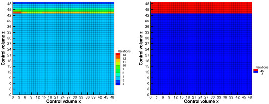
Figure 2. Number of iterations carried out for a spatial mesh 50 × 50 cells using a Newton–Raphson+regula–falsi (left frame) and Newton–Raphson+bisection (right frame). The color of each cell in the mesh is related to the number of iterations carried out.

Since the heat capacity of ice is around half the heat capacity of liquid water, we used in this work the values $k_1=0.5$, $k_2=1$. Other values taken are ${ϵ}_0=0.01$ and $L=330$, which refer to the latent heat of fusion of water measured in KJkg${}^{-1}$. The algorithm for the nonlinear solver is as follows.

Algorithm 2 Nonlinear solver.

1: Prescribed $maxiterN$, $maxiterRF$, $tolmax$, $T_s^{\left(1\right)}$ 2: $tol\leftarrow 2·tolmax$; 3: $iter\leftarrow 1$ 4: while$(iter\le maxiterN$ & $tol>tolmax)$ do 5:     $F\leftarrow \gamma \left(T_s^{\left(iter\right)}\right)-{\gamma }^{n+1}\left(T_s\right)$$using$ (10) 6:     $DF\leftarrow {\gamma }^{\prime }\left(T_s^{\left(iter\right)}\right)$ 7:     $T_s^{(iter+1)}\leftarrow T_s^{\left(iter\right)}-\frac{F}{DF}$ 8:     $tol\leftarrow abs(T_s^{(iter+1)}-T_s^{\left(iter\right)})$ 9:     $iter\leftarrow iter+1$ 10: end while 11: if$(iter>maxiterN)$then 12:     $Call$$Function$$Regula-falsi$ 13: end if 14: $\mathbf{Function}$$Regula-falsi:$ 15: Prescribed $T_{s,a}$, $T_{s,b}$$such$$that$$T_{s,a}·T_{s,b}<0$, $tolmax$, $maxiterRF$ 16: $iter\leftarrow 1$ 17: while$(iter\le maxiterRF$ & $tol>tolmax)$ do 18:     $T_s^{\left(iter\right)}\leftarrow \frac{T_{s,a}Fb-T_{s,b}Fa}{Fb-Fa}$ 19:     $Fm\leftarrow \gamma \left(T_s^{\left(iter\right)}\right)-{\gamma }^{n+1}\left(T_s\right)$ $using$ (10) 20:     $Fa\leftarrow \gamma \left(T_{s,a}\right)-{\gamma }^{n+1}\left(T_s\right)$ $using$ (10) 21:     $Fb\leftarrow \gamma \left(T_{s,b}\right)-{\gamma }^{n+1}\left(T_s\right)$ $using$ (10) 22:     if $(Fm·Fa<0)$ then 23:         $T_{s,b}\leftarrow T_s^{\left(iter\right)}$ 24:     else 25:         $T_{s,a}\leftarrow T_s^{\left(iter\right)}$ 26:     end if 27:     $tol\leftarrow abs\left(T_s^{\left(iter\right)}\right)$ 28:     $iter\leftarrow iter+1$ 29: end while 30: $T_s^{n+1}\leftarrow T_s^{\left(iter\right)}$

4. Numerical Examples

The mathematical model under study is a coupled model formed by a vegetation cover and soil underneath it, describing the evolution of temperature. The main processes and equations are described in Section 2. The system (36) represents the full coupled model.

$$\left\{\begin{array}{cc}\hfill {\displaystyle C_v\frac{\partial T_v}{\partial t}-\frac{\partial }{\partial x}\left(K_{H0}\frac{\partial T_v}{\partial x}\right)+K_V\frac{\partial T_s}{\partial n}=F_v,}\hfill & \hfill {\displaystyle x\in (-l,l),t>0}\hfill \\ \\ \hfill {\displaystyle \frac{\partial \gamma \left(T_s\right)}{\partial t}-\frac{\partial }{\partial x}\left(K_H\frac{\partial T_s}{\partial x}\right)-\frac{\partial }{\partial z}\left(K_V\frac{\partial T_s}{\partial z}\right)=F_s,}\hfill & \hfill {\displaystyle (x,z)\in (-l,l)\times (-H,0),t>0}\hfill \\ \hfill {\displaystyle \frac{\partial T_v}{\partial x}(-l,t)=\frac{\partial T_v}{\partial x}(l,t)=0,}\hfill & \hfill {\displaystyle t>0}\hfill \\ \hfill {\displaystyle \frac{\partial T_s}{\partial x}(-l,z,t)=\frac{\partial T_s}{\partial x}(l,z,t)=\frac{\partial T_s}{\partial z}(x,-H,t)=0,}\hfill & \hfill {\displaystyle x\in (-l,l),t>0}\hfill \\ \hfill {\displaystyle T_s(x,0,t)=T_v(x,t);}\hfill & {\displaystyle x\in (-l,l),t>0}\hfill \\ \hfill {\displaystyle T_v(x,0)=C_1·exp(-80·si{n}^2\left(x^4\right))+C_2,}\hfill & \hfill {\displaystyle x\in (-l,l)}\hfill \\ \hfill {\displaystyle T_s(x,z,0)=C_1·exp(-80·si{n}^2\left(x^4\right)-80z^2)+C_2,}\hfill & \hfill {\displaystyle (x,z)\in (-l,l)\times (-H,0).}\hfill \end{array}\right.$$

(36)

In problem (36), $C_1$ and $C_2$ are constant values. The spatial domain considered is $(-l,l)\times (-H,0)$. The numerical simulation is conducted applying a finite volume method with seventh-order WENO reconstruction in space and RK3-TVD for time integration, as described in Section 3. As previously detailed, the nonlinearity appearing due to the latent heat of fusion $\gamma \left(T_s\right)$ is solved by Newton–Raphson’s numerical scheme combined with regula–falsi technique. The algorithm followed is described in Section 3.2. The spatial mesh is formed by $50\times 50$ control volumes. The size of the time step is computed as $\Delta t=min(CFL\times \frac{\Delta x^2}{K_{H0}},CFL\times \frac{\Delta x^2}{K_H},CFL\times \frac{\Delta z^2}{K_V})$, where $CFL=0.35$ for stability reasons. Concerning heat conduction, we take $K_{H0}=0.01$, $K_H=0.03$, and $K_V=0.03$.

In Figure 3, results for the evolution of the temperature in the vegetation layer are shown for time $t=0.15$. We took $C_1=35$ and $C_2=290$ in the initial condition of the model (36), an ambient temperature of $T_a=313+sin\left(t\right)$ for the results shown in the left frame, and $T_a=265+sin\left(t\right)$ for the results displayed in the right frame. The curves displayed are labeled as follows: Without coupling, which means that $\frac{\partial T_s}{\partial n}$ is removed in (1); With coupling, which means that $\frac{\partial T_s}{\partial n}$ is considered. It can be observed that when the temperatures are low (right frame of Figure 3), the coupled case gives rise to higher temperatures than the uncoupled one; on the other hand, when the temperatures are higher, the coupled case gives rise to lower temperatures than the uncoupled one (left frame of Figure 3). This is due to the effect of the top soil, which can be considered as a major insulator of heat (see [4]) and may have an important influence on the vegetation cover.

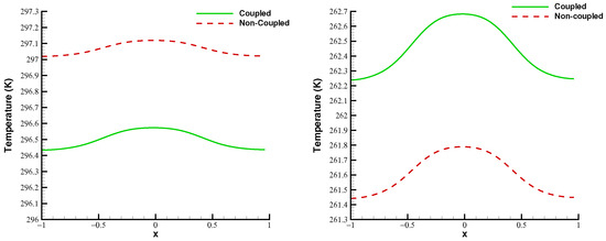
Figure 3. Temperature at the vegetation layer ($T_v$). Output time t = 0.5. Without coupling means that $\frac{\partial T_s}{\partial n}$ is removed in (1) while With coupling means that $\frac{\partial T_s}{\partial n}$ is considered. In both cases, we used $C_1=35$ and $C_2=290$, with the ambient temperature being $T_a=313+sin\left(t\right)$ (left frame) and $T_a=265+sin\left(t\right)$ (right frame).

We study now the space-time evolution within the bottom soil. The plots displayed in Figure 4 show the distribution of temperature $T_s$ inside the ground solving the problem (36) for several output times.

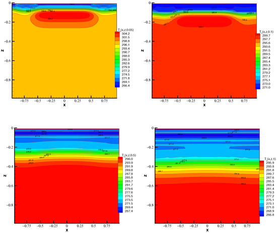
Figure 4. Temperature in the soil ($T_s$) for output times = $0.05$ (top left), $0.1$ (top right), $0.5$ (bottom left), and 1 (bottom right) when the ambient temperature is $T_a=290+sin\left(t\right)$ for $C_1=35$ and $C_2=298$ in the initial condition of (36). The depth is represented by the coordinate z.

It can be observed that the strongest variations of temperature take place in the top soil, close to the surface; whereas, when advancing in depth, the temperature tends to an approximate constant value, which agrees with practical experience. In this case, the values used are $C_1=35$ and $C_2=298$ in the initial condition of the problem (36) and the ambient temperature is $T_a=290+sin\left(t\right)$. In this example and the subsequent ones, we considered $\frac{\partial T_s}{\partial n}$ in the vegetation cover equation. The effect of the latent heat of fusion in the different plots can also be observed since, around 273 K, the temperature remains approximately constant as the phase change is taking place.

In Figure 5, the evolution of the temperature $T_s$ in the bottom soil is depicted with depth for different ambient temperatures $T_a$. The results show that as depth increases, the temperature attains a value close to the constant 298 K, independent of the ambient temperature considered. In this case, the values $C_1=35$ and $C_2=298$ are used in the initial condition of problem (36).

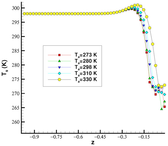
Figure 5. Soil temperature distribution with depth ($T_s(0,z,0.2)$) for different values of the ambient temperature $T_a$.

The results displayed indicate that seasonal variations in the ambient temperature do not have an effect on the temperature of the bottom soil as depth increases, since the temperature remains close to a constant value. This fact has been verified in all the numerical examples presented. It also agrees with [28], where it is also stated that a similar situation takes place universally around the world.

In the last numerical example, results with and without latent heat of fusion are shown. To proceed, the coefficients $C_1=6$ and $C_2=298$ are introduced in the initial condition of the system (36) and, as ambient temperature, the function $T_a=265+sin\left(t\right)$ has been considered. Since the temperature varies between values lower and higher than 273 K, the effect of the latent heat of fusion is clearly visible. It can be appreciated, in the top-left panel of Figure 6, that when the temperature in the soil is around 273 K, it remains approximately constant since the energy goes to the phase change instead of to increasing the temperature. This effect has also been studied in climate models, such as those reported in [29].

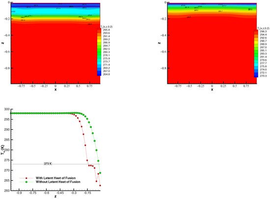
Figure 6. Temperature in the soil ($T_s$) for output time = $0.2$ when the ambient temperature is $T_a=265+sin\left(t\right)$ and $C_1=6$ and $C_2=298$ in the initial condition of (36). The depth is represented by the coordinate z. Top: temperature in the soil considering latent heat (left panel) and without latent heat (right panel). Bottom: evolution of temperature in the soil ($T_s$) cutting with $x=0$.

In the top-right panel, the effect of the latent heat of fusion is not considered. This means that $\gamma \left(T_s\right)=T_s$ is used in Equation (36) and the plot shows that the variation of temperature is smoother than when latent heat of fusion is taken into consideration.

The bottom panel represents a cut with $x=0$ of the plots above for a clearer comparison of the cases with and without latent heat of fusion. It can be observed that there is a decrease in the temperature in the vicinity of the surface but, as depth increases, the temperature starts to rise, with a similar profile to the situation without latent heat of fusion ($\gamma \left(T_s\right)=T_s$). When the phase change temperature is reached, around $T_s$ = 273 K, the temperature slows its growth as the phase change occurs.

5. Conclusions and Discussion

In this work, we introduced a mathematical model describing the interaction between a $1D$ vegetation cover and the $2D$ ground underneath this cover. The model is coupled, in the sense that vegetation cover is a dynamic and diffusive boundary condition for the $2D$ domain. The main heat exchange processes take place in the top soil, which is the part of the soil that is closer to the vegetation cover. The equation of the vegetation cover includes a normal derivative, accounting for heat conduction from the soil to the vegetation. The model also takes into account the water phase change, which is described by the function $\gamma \left(T_s\right)$, where $T_s$ is the temperature in the soil. Therefore, heat capacity is not a constant, but a function of the temperature of the soil. This nonlinearity is resolved by means of a Newton–Raphson’s technique combined with a regula–falsi one (which acts automatically when Newton–Raphson’s scheme fails to converge).

The main interactions between the vegetation and the soil take place in a thin region close to the surface, the top soil.

The mathematical model is solved using a finite volume numerical scheme, with a third-order TVD Runge–Kutta scheme for time integration and a seventh-order WENO approach for spatial reconstruction. These techniques are very efficient for solving this type of problems.

The results obtained show that the main temperature variations take place in the vicinity of the surface—namely, the top soil—whereas as depth increases the temperature tends to a constant value, as expected. This conclusion agrees with the real situation as reported in references on this topic.

Further research will include the consideration of water content and moisture in the soil, as well as taking into account different types of plants. In addition, it will be interesting to introduce the effect of precipitation, as it may affect the integrity of the vegetation cover.

References

- Sailor, D. A green roof model for building energy simulation programs. Energy Build. 2008, 40, 1466–1478. [Google Scholar] [CrossRef]
- Vilar, M.; Tello, L.; Hidalgo, A.; Bedoya, C. An energy balance model of heterogeneous extensive green roofs. Energy Build. 2021, 250, 111265. [Google Scholar] [CrossRef]
- Andújar Márquez, J.M.; Martínez Bohórquez, M.; Gómez Melgar, S. Ground Thermal Diffusivity Calculation by Direct Soil Temperature Measurement. Application to very Low Enthalpy Geothermal Energy Systems. Sensors 2016, 16, 306. [Google Scholar] [CrossRef] [PubMed] [Green Version]
- Onwuka, B.; Mang, B. Effects of soil temperature on some soil properties and plant growth. Adv. Plants Agric. Res. 2018, 8, 34–37. [Google Scholar] [CrossRef]
- Singh, R.K.; Sharma, R.V. Numerical analysis for ground temperature variation. Geotherm. Energy 2017, 5, 22. [Google Scholar] [CrossRef] [Green Version]
- Santos, F.; Abney, R.; Barnes, M.; Bogie, N.; Ghezzehei, T.A.; Jin, L.; Moreland, K.; Sulman, B.N.; Berhe, A.A. Chapter 9-The role of the physical properties of soil in determining biogeochemical responses to soil warming. In Ecosystem Consequences of Soil Warming; Mohan, J.E., Ed.; Academic Press: Cambridge, MA, USA, 2019; pp. 209–244. [Google Scholar] [CrossRef]
- Frankenstein, S.; Koenig, G.G. Fast All-Season Soil STrength (FASST); ERDC/CRREL TR-04-25 2004; U.S. Army: Washington, DC, USA, 2004. [Google Scholar]
- Tello, J.I.; Tello, L.; Vilar, M.L. On the Existence of Solutions of a Two-Layer Green Roof Mathematical Model. Mathematics 2020, 8, 1608. [Google Scholar] [CrossRef]
- Deardorff, J.W. Efficient Prediction of Ground Surface Temperature and Moisture, With Inclusion of a Layer of Vegetation. J. Geophys. Res. 1978, 83, 1889–1903. [Google Scholar] [CrossRef] [Green Version]
- Ramirez, J.A.; Senarath, S.U. Statistical-dynamical parameterization of interception and land surface-atmosphere interactions. J. Clim. 2000, 13, 4050–4063. [Google Scholar] [CrossRef]
- Henderson-Sellers, B. A new formula for latent heat of vaporization of water as a function of temperature. Q. J. R. Meteorol. Soc. 1984, 110, 1186–1190. [Google Scholar] [CrossRef]
- Gottlieb, S.; Shu, C.W. Total Variation Diminishing Runge-Kutta schemes. Math. Comput. 1998, 67, 73–85. [Google Scholar] [CrossRef] [Green Version]
- Hidalgo, A.; Tello, L. Numerical Approach of the Equilibrium Solutions of a Global Climate Model. Mathematics 2020, 8, 1542. [Google Scholar] [CrossRef]
- Godunov, S. A Difference Scheme for Numerical Solution of Discontinuous Solution of Hydrodynamic Equations. Math. Sbornik 1959, 47, 271–306. [Google Scholar]
- Harten, A. High resolution schemes for hyperbolic conservation laws. J. Comput. Phys. 1983, 49, 357–393. [Google Scholar] [CrossRef] [Green Version]
- Harten, A.; Engquist, B.; Osher, S.; Chakravarthy, S.R. Uniformly High Order Accurate Essentially Non-oscillatory Schemes, III. J. Comput. Phys. 1997, 131, 3–47. [Google Scholar] [CrossRef]
- Dumbser, M.; Enaux, C.; Toro, E.F. Finite volume schemes of very high order of accuracy for stiff hyperbolic balance laws. J. Comput. Phys. 2008, 227, 3971–4001. [Google Scholar] [CrossRef]
- Dumbser, M. Arbitrary high order PNPM schemes on unstructured meshes for the compressible Navier—Stokes equations. Comput. Fluids 2010, 39, 60–76. [Google Scholar] [CrossRef]
- Dumbser, M.; Hidalgo, A.; Castro, M.; Parés, C.; Toro, E.F. FORCE schemes on unstructured meshes II: Non-conservative hyperbolic systems. Comput. Methods Appl. Mech. Eng. 2010, 199, 625–647. [Google Scholar] [CrossRef]
- Jiang, G.S.; Shu, C.W. Efficient Implementation of Weighted ENO Schemes. J. Comput. Phys. 1996, 126, 202–228. [Google Scholar] [CrossRef] [Green Version]
- Dumbser, M.; Zanotti, O.; Hidalgo, A.; Balsara, D.S. ADER-WENO finite volume schemes with space–time adaptive mesh refinement. J. Comput. Phys. 2013, 248, 257–286. [Google Scholar] [CrossRef] [Green Version]
- Dumbser, M.; Hidalgo, A.; Zanotti, O. High order space–time adaptive ADER-WENO finite volume schemes for non-conservative hyperbolic systems. Comput. Methods Appl. Mech. Eng. 2014, 268, 359–387. [Google Scholar] [CrossRef] [Green Version]
- Titarev, V.; Toro, E. Finite-volume WENO schemes for three-dimensional conservation laws. J. Comput. Phys. 2004, 201, 238–260. [Google Scholar] [CrossRef]
- Castro, M.J.; Semplice, M. Third- and fourth-order well-balanced schemes for the shallow water equations based on the CWENO reconstruction. Math. Comput. Model. 2019, 89, 304–325. [Google Scholar] [CrossRef]
- Cravero, I.; Puppo, G.; Semplice, M.; Visconti, G. CWENO: Uniformly accurate reconstructions for balance laws. Math. Comp. 2018, 87, 1689–1719. [Google Scholar] [CrossRef] [Green Version]
- Semplice, M.; Travaglia, E.; Puppo, G. One- and Multi-dimensional CWENOZ Reconstructions for Implementing Boundary Conditions Without Ghost Cells. Commun. Appl. Math. Comput. 2021, 17, 609–618. [Google Scholar] [CrossRef]
- Baeza, A.; Bürger, R.; Mulet, P.; Zorío, D. An Efficient Third-Order WENO Scheme with Unconditionally Optimal Accuracy. SIAM J. Sci. Comput. 2020, 42, A1028–A1051. [Google Scholar] [CrossRef]
- Selker, J.; Or, D. Soil Hydrology and Biophysics; Oregon State University: Corvallis, OR, USA, 2019. [Google Scholar]
- Díaz, J.I.; Hidalgo, A.; Tello, L. Multiple solutions and numerical analysis to the dynamic and stationary models coupling a delayed energy balance model involving latent heat and discontinuous albedo with a deep ocean. Proc. R. Soc. A 2014, 470, 20140376. [Google Scholar] [CrossRef] [PubMed] [Green Version]
Publisher’s Note: MDPI stays neutral with regard to jurisdictional claims in published maps and institutional affiliations. |
© 2022 by the authors. Licensee MDPI, Basel, Switzerland. This article is an open access article distributed under the terms and conditions of the Creative Commons Attribution (CC BY) license (https://creativecommons.org/licenses/by/4.0/).