Chaotic Model of Brownian Motion in Relation to Drug Delivery Systems Using Ferromagnetic Particles

Abstract

Deterministic and stochastic models of Brownian motion in ferrofluids are of interest to researchers, especially those related to drug delivery systems. The Brownian motion of nanoparticles in a ferrofluid environment was theoretically analyzed in this research. The state of the art in clinical drug delivery systems using ferromagnetic particles is briefly presented. The motion of the nanoparticles in an external field and as a random variable is elaborated by presenting a theoretical model. We analyzed the theoretical model and performed computer simulation by using Maple software. We used simple low-dimensional deterministic systems that can exhibit diffusive behavior. The ferrofluid in the gravitational field without the presence of an external magnetic field in the xy plane was observed. Control parameter p was mapped as related to the fluid viscosity. Computer simulation showed that nanoparticles can exhibit deterministic patterns in a chaotic model for certain values of the control parameter p. Linear motion of the particles was observed for certain values of the parameter p, and for other values of p, the particles move randomly without any rule. Based on our numerical simulation, it can be concluded that the motion of nanoparticles could be controlled by inherent material properties and properties of the surrounding media, meaning that the delivery of drugs could possibly be executed by a ferrofluid without an exogenous power propulsion strategy. However, further studies are still needed.

1. Introduction

Models of Brownian motion, both stochastic and deterministic, have been of interest to researchers for a long time [1]. Lucretius considered in 60 BC that the movement of dust particles in the air is caused by the movement of small invisible particles. The chaotic movements of coal particles in alcohol were described by Ingenhousz in 1785. In 1827, the botanist Brown observed the movement of pollen in water under a microscope. A mathematical description of Brown’s movement was given in 1880 by Thiele and in 1900 by Bachelier. In 1905, Einstein developed a stochastic theory of Brownian motion [2], which Perrin experimentally proved in 1909. Langevin in 1908 used a stochastic differential equation to describe changes in macroscopic variables. In 1965, Mori described transport, collective motion and Brownian motion within statistical-mechanical theory [3]. Saffman and Delbruck investigated Brownian motion in 1975 in biological membranes. Caldeira and Legget investigated the quantum Brownian motion of 1983 [4].

Fujisaka, Grossmann, Thomae and Geisel from 1982 to 1985 wanted to form a dynamic theory of Brownian motion [5]. In 1998, Gaspard and his associates experimentally proved microscopic chaos [6]. In 2005, Cecconi attempted to determine the microscopic nature of diffusion by data analysis [7]. Since 2011, Brownian motion in superfluids has been considered. There are various studies of Brownian motion and stochastic and chaotic models are observed, and the nature of this movement is a difficult question and the answer is not determined by the character of the model [8,9].

The first definition of Brownian motion was related to stochastic process [10], in relation to a wide range of different real stochastic processes, and represented by the Wiener process, which describes continuous-time stochastic process with real values [11]. Brownian motion can be observed as stochastic or deterministic in chaos theory, based on the deterministic equations that describe stochastic phenomena [11], but the governing parameters that might provide a full replication of the experiment are difficult to determine or define. Recent computer simulation experiments have shown the possibility to model the chaotic system as a stochastic one, by controlling simulation parameters and initial conditions [11]. Such an approach has enabled research on how to govern the chaotic system (and determine governing parameters) through the study of particle trajectories that have random motion, that is, by using deterministic equations to reproduce random behavior [11].

The generation of deterministic Brownian motion is possible through additional degrees of freedom in the Langevin equation of the phenomenological system of particle mixing and agitation in fluids [12]. Another study [13] replicated Brownian motion by using a fully deterministic set of differential equations and applied it to a real problem of electronic circuit implementation. Their deterministic model showed that some variables within the model can enable modeling of the circuit dynamics as a stochastic Brownian behavior [13]. There are numerous real systems that exhibit Brownian behavior, and modeling such systems by deterministic systems (without random components) is an important area in recent research, including drug delivery systems [13]. An analysis of 126 different combinations of governing parameters is given in [13], and around 10% of those cases involved deterministic Brownian-like motion. They obtained stochastic or deterministic Brownian motion based on the initial setup conditions (assigned initial parameters values for circuit implementation) [13].

Ferrofluids are a suspension of small particles of 10 nm, each of which contains one permanent ferromagnetic domain [14]; thus, each particle is a permanent magnet, which, in the absence of an external magnetic field, rotates randomly under the action of Brown’s forces, which are strong due to the small particle size [15]. In ferrofluids, dipoles exist without fields and rotate randomly by Brownian motion [16]. Ferrofluids are interesting magnetic fluids that can be controlled by an external magnetic field [17]. There are several applications for ferrofluids in industrial as well as technological fields such as magnetic memory, inkjet printers, magnetic seals, etc. [18]. They are known for their biomedical applications such as magnetic resonance contrast agents [19], hyperthermia [20], targeted drug delivery to tumor and cancer cells, antibacterial activity, etc. [21,22].

Numerical computational simulations have emerged in the past decade as powerful tools for the analysis and prediction of the material physical behavior at macro/micro and nano scales, with extensive research on applied models and software solutions. Thermal conductivity of fluids is the most influential factor for the fluid behavior, and different approaches to estimate or predict it for novel nanofluids have been studied using mathematical models [23,24,25] or experimentally based models [26]. For example, models related to the rheological properties of hybrid non-Newtonian nanofluids are important, since it is proven that with the increase in volume fractions of nanoparticles, the effect of temperature increase is more influential, leading to the non-Newtonian behavior of the nanofluid and also having a strong effect on viscosity [26].

A mathematical model was developed, using SigmaPlot software, to study the thermal conductivity of nanofluids, through the study of different volume fractions of ternary hybrid nanofluids and mono and binary hybrid nanofluids [23]. This model correlated volume fractions of different nanofluids and resulting thermal conductivity in order to provide a tool for the estimation of thermal conductivity of a ternary hybrid nanofluid [23]. Thermal properties of DNA structure in water fluid were estimated by using equilibrium and non-equilibrium molecular dynamics approaches and LAMMPS (Large-scale Atomic/Molecular Massively Parallel Simulator) software [24]. Another work on the prediction of the thermal conductivity of hybrid Newtonian nanofluid proposed an algorithm to solve the problem in the Artificial Neural Network (ANN) [25] that considered the volume fraction of nanoparticles and temperature.

This paper studies the possibility to use and influence Brownian motion to produce patterned trajectories of particles in a diffusive motion of the ferrofluid, aiming to assist in more efficient drug delivery nanofluid systems. A chaotic model of Brownian motion was theoretically analyzed and simulated by using Maple software. The chaotic model was mapped with an introduced control parameter, p, which depends on the viscosity coefficient and particle mass and size, in analogy with the Langevin equation. The ferrofluid in the gravitational field without the presence of an external magnetic field in a two-dimensional model was observed.

2. Materials and Methods

2.1. Brownian Motion

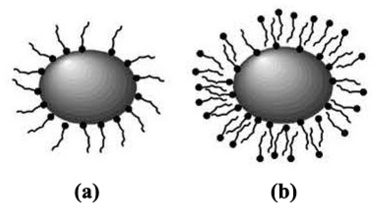
Numerous experiments show that there is a constant internal movement in every substance. This internal movement is in fact the movement of the molecules that make up the observed substance. This movement of molecules is unregulated, never stops and depends only on temperature. The phenomenon discovered by Brown directly indicates the stochastic nature of the movement of molecules, where the same initial condition will not replicate the resulting motion (the same trajectory in time). Using a microscope, it was observed that very small particles floating in a liquid are in a state of continuous stochastic motion, and the smaller the particles, the faster they move [27]. This motion, called Brownian motion, never stops, does not depend on any external cause and is a manifestation of the particles’ motion due to colliding with surrounding molecules of fluid and internal energy of matter: the potential energy of all the particles and thermal energy of moving particles (kinetic energy), which is correlated to the temperature and number of particles (mass). When they collide with a solid body, liquid molecules, which are constantly moving, are subjected to a certain amount of movement. If the body is in a liquid and has larger dimensions, the number of molecules that come across it from all sides is also very large, and their shocks are compensated at any time and the body remains practically motionless [28].

If the body is small, such compensation may be incomplete: it can accidentally hit one side of the body with a much larger number of molecules than the other, causing the body to move [28]. It is a movement performed by Brown’s particles under the action of chaotic blows of molecules. Brown’s particles have several billion times the mass of individual molecules and their velocities are very low compared to the speeds of molecules, but their movement can be observed with a microscope. In this way, too, a substance not only has a granular structure—that is, it consists of individual separate parts—but it also consists of particles that are constantly moving.

2.2. Ferrofluid

A magnetic colloidal particle, also known as a ferrofluid, is a colloidal suspension of single-domain magnetic particles, typically about 10 nm in size, dispersed in a liquid carrier [15,16]. The liquid carrier can be polar or non-polar [14]. Since the 1960s, when ferrofluid was initially synthesized, its technical and medical applications have not stopped growing [18]. Ferrofluid differs from ordinary magnetorheological fluids used for shock absorbers, brakes and clutches, formed by micron-sized particles dispersed in oil [18]. In magnetorheological fluid, the application of a magnetic field increases the viscosity, so that for a sufficiently strong field, it can behave like a solid [16,18]. On the other hand, ferrofluid retains its fluidity even if it is exposed to a strong magnetic field. Ferrofluids are optically isotropic, but in the presence of an external magnetic field, they show induced birefringence [29]. Wetting of certain substrates can also cause bifurcation in thin ferrofluid layers. To avoid agglomeration, the magnetic particle should be coated with a shell of a suitable material [30,31]. In relation to the coating, ferrofluid is divided into two main groups: surfactant, if the coating is a surfactant molecule, and ionic, if it is an electric shell [30,31].

Colloidal suspensions of magnetic particles in liquids that have the ability to magnetize in an external magnetic field are called ferrofluids [32]. These are magnetic materials in liquid form. The liquid can be water or an organic solution in which ferromagnetic or ferrimagnetic particles are dispersed. The particles are most often hematite, Fe₂O₃, or magnetite, Fe₃O₄, and they need to be stabilized due to high surface energy by adding a polymer or ionic component (surfactant). Usually, such stable particles are about 10 nm in diameter, and their surface energy is reduced by long-chain surfactants which, thanks to the long chains, prevent agglomeration, or the same charge on the surface of magnetic particles leads to a mutual repulsion, preventing agglomeration [30]. Ferrofluid particles do not precipitate even for a long time, they do not agglomerate and they do not separate from liquids even by applying an extremely strong magnetic field. The combination of the liquid phase and the magnetic behavior makes it possible to manipulate the fluid by changing its position using an external magnetic field [32].

To avoid agglomeration, ferrofluid particles are coated [30,31]. Depending on the coating, ferrofluids are divided into two groups: surfactant-coated ferrofluids and electrostatically stabilized ferrofluids [31]. Surfactant-coated ferrofluids contain magnetic particles coated with amphiphilic molecules such as oleate to prevent aggregation. Spherical repulsion between particles acts as a physical barrier that keeps the particles in solution and stabilizes the colloid. If the particles are dispersed in a nonpolar phase, such as oil, the polar head of the surfactant is attached to the surface of the particles, and the hydrophobic chain is in contact with the liquid (Figure 1a). If the particles are dispersed in the polar phase such as water, a two-layer coating of the particles is required to form a hydrophilic layer around them (Figure 1b).

One of the fastest developed areas of research is one in which nanotechnology, biology and medicine intertwine. According to many experts, the application of nanotechnology in medicine, better known as nanomedicine, will lead to a revolution in the field of targeted drug delivery systems [33,34], disease diagnosis, bioengineering and the improvement of contrast agents in magnetic resonance imaging. The term “teragnostics” is usually used in this context, which, as the name itself implies, is a synthesis of diagnostics and therapy. The localization of ferrofluids by the applied magnetic field gives an interesting application of ferrofluids in medicine. A lot of research has been dedicated to the use of ferrofluids as a system for targeted delivery of drugs used in chemotherapy [35]. A drug is injected into tumor carcinomas and retained there for some time by a magnetic field. The amount of medicine needed is much less than the amount of medicine that would be needed to distribute the medicine throughout the body. After turning off the magnetic field, the drug will disperse in the body, but since it is a much smaller amount, there are practically no side effects.

The ability of ferrofluid to absorb the energy of electromagnetic waves at a frequency different from the frequency at which water absorbs energy allows heating of the localized part of the tissue where the ferrofluid is injected (for example, tumors) without heating the surrounding tissues. This phenomenon is called hyperthermia. Hyperthermia is one of the methods used in cancer therapy that is based on increasing the temperature of tumor tissue above 41 °C. As a result, the function of tumor cells is disturbed and they die. Magnetic hyperthermia is based on the effect of releasing heat when magnetic nanoparticles are found in a changing magnetic field. Magnetic nanoparticles can be successfully localized in tumor tissue, which allows heating only in the desired place. In therapy, these particles are most often used in colloidal form. It is possible to bind chemotherapy drugs or radionuclides to these particles and thus achieve a combined effect.

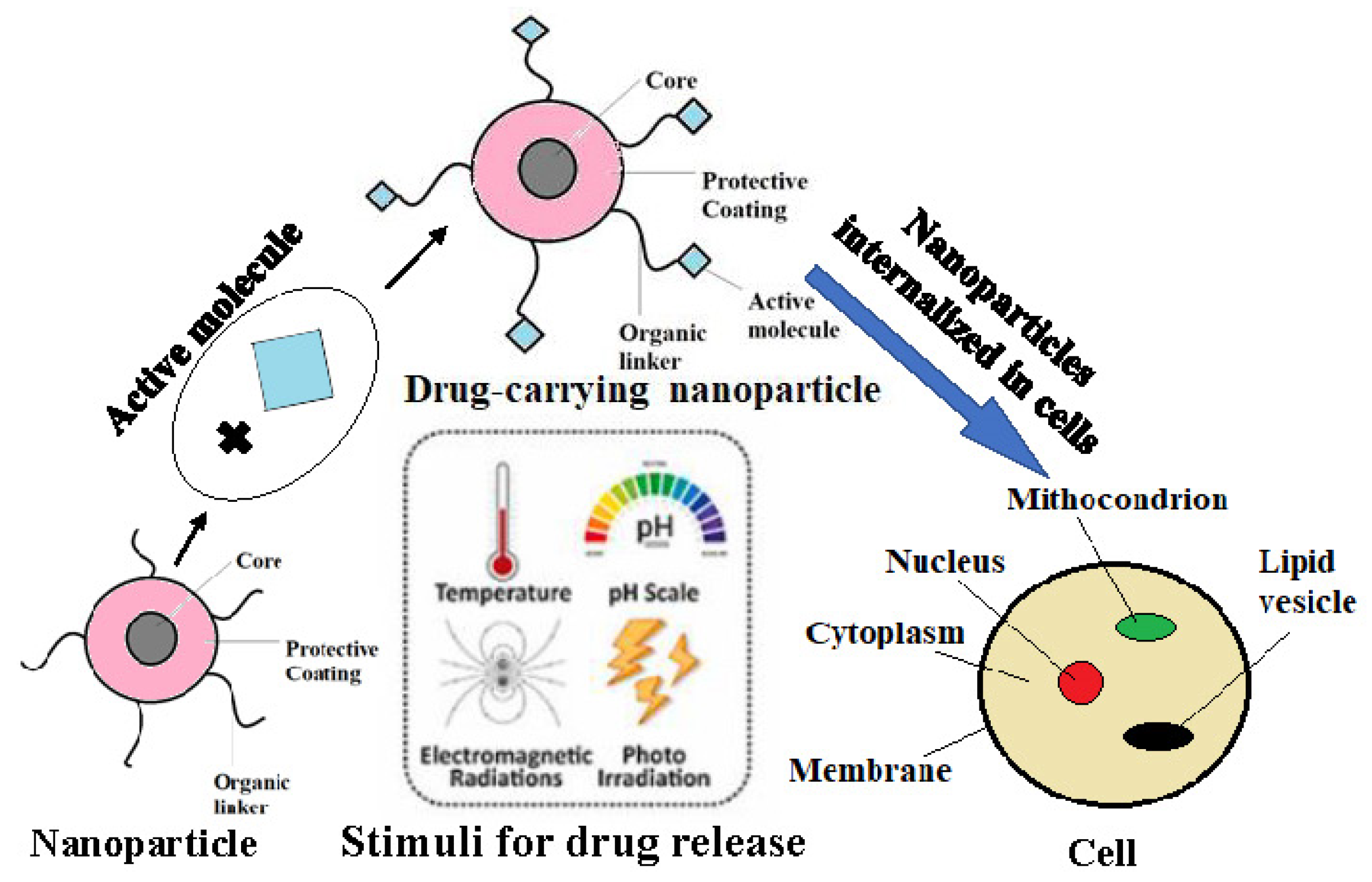
2.3. State of the Art in Clinical Drug Delivery Systems Using Ferromagnetic Particles

Drug delivery systems based on nanotechnology have improved the delivery of drugs due to their changes in pharmacokinetics, enabling a longer half-life of the drug in the bloodstream and reducing toxicity [36]. Magnetic nanoparticles play an important role in the diagnosis and treatment of diseases such as cancer, heart and neurological diseases [37]. These particles are often used in the targeted delivery of medically active substances because they deliver the drug to the desired place via tissue magnetic absorption or strong ligand–receptor interaction [38].

The drug–carrier complex can be administered intravenously or by arterial injection [39]. It can also be administered orally, but the main problem with such administration is the delivery of peptides and proteins due to their breakdown in gastric acid, low absorption and first-pass metabolism through the liver [40].

If a drug is delivered by a magnetic field, the gradient of the external magnetic field associated with the magnetic field within human tissues enables the transfer and accumulation of magnetic nanoparticles in the body [41]. However, there are a number of intracellular and extracellular barriers that can be limiting factors. One of the possible solutions is covering the surface of nanoparticles with biocompatible materials (different organic and inorganic compounds) [37]. Coating the surface of nanoparticles increases the half-life of the drug by delaying clearance [38]. Macrophages take up uncoated nanoparticles at a rate that depends on their functional surface, size and hydrophilicity, followed by clearance in the liver and spleen. Plasma proteins bind to the surface of nanoparticles, accelerating phagocytosis. Coatings enable the slowing down of detection by macrophages and thus reduce clearance. For this purpose, the most often used is polyethylene glycol (PEG), the attachment of which provides a “stealth” protective effect. PEG is suitable for this purpose because it shows low toxicity and immunogenicity and is excreted by the kidneys [42]. In addition, surface coating enables covalent binding of biomolecules such as antibodies and proteins and their transport to the target tissue. It is necessary that these coatings be sensitive to the change in pH value, which would enable the controlled release of the drug [43]. Drug release can be stimulated by chemical radiation, mechanical forces and magnetic hyperthermia [38].

Figure 2 shows the structure of a magnetic nanoparticle carrying the active molecule on the surface.

The most important characteristics of nanoparticles used for drug delivery are intrinsic magnetic properties, the shape and size of nanoparticles, non-toxicity, stability in water, surface charge and coating. Many magnetic materials with ideal magnetic properties, such as cobalt or chromium, are very toxic and cannot be used in medicine, while materials based on iron oxide (magnetite or maghemite) are safe. In addition to low toxicity, these nanoparticles show high stability against degradation [38]. The size of the particles is such that they allow entry into biological structures, and it varies from 3 to 30 nm [41].

This method can be applied to solid tumor mass, neoplasms with metastases and tumors that are in the early phase of cell growth. Treatment would involve the application of particles that specifically recognize clusters of cancer cells, carrying a medically active substance that will act [44].

2.4. Motion of Particles in an External Field and as a Random Variable

Nanoparticles move after collision with smaller water molecules. Smaller water molecules come across the nanoparticle from all directions and collide with it, thus imparting their momentum to it. When at some point after such a collision a particle receives a momentum in that direction, it starts to move in that direction, until another water molecule collides with it and gives it its momentum by collision. If in the field of classical mechanics, this mode of motion is, in principle, deterministic and there is a corresponding Hamiltonian [45]. In reality, due to the large number of water molecules that interact with each other and with the nanoparticle, and due to the unknown initial conditions, such a system cannot be described using the Hamiltonian in practice, i.e., it is impossible to say with certainty how much and in which direction the particle will move in at some point. On the contrary, a shift in any direction is equally probable (this can be seen intuitively from the symmetry of the system). That is why the tool of statistical physics is used to study such a system. Due to the large number of water molecules that make up the system, instead of observing the microscopic effect on the nanoparticle of each of them, one can observe their “total” macroscopic effect after some time. After repeating such an experiment several times with the same initial conditions (as much as it can be controlled, e.g., placing a nanoparticle with the same physical values in the same place), a different value is obtained for the total macroscopic displacement of the nanoparticle after a certain time. This gives an empirical distribution of the probability of the total movement of a nanoparticle, and therefore, instead of looking at exactly how much a nanoparticle will move at a given moment, one can look at the probability that the particle will move by a certain value at a given moment.

A fluid containing a large number of particles (Brownian particles) and moving in one dimension is observed. The density is given by n(x, t), where n is the particle density, x is the position coordinate and t is the time. Brownian motion over time makes the density uniform. The flow of particles during diffusion j_d is defined by:

$$j_d\left(x,t\right)=-D\frac{\partial n\left(x,t\right)}{\partial x}$$

(1)

The flow of particles causes a change in density in time according to the continuity equation:

$$\frac{\partial n\left(x,t\right)}{\partial t}=-\frac{\partial j_d\left(x,t\right)}{\partial x}=D\frac{{\partial }^{2}n\left(x,t\right)}{\partial x^2}$$

(2)

In the equation, D [m²/s] is the diffusion constant (it depends on the type of particle material), and the given equation is the diffusion equation. The flow of particles is opposite to the direction of the density gradient and the flow direction is from the area of higher density to the area of lower density.

A uniform force field (gravitational field) acts on the Brownian particles. The stated field accelerates the particles until the velocity reaches a certain limiting velocity, ug, and where the sum of the forces acting on the particle, the force field, F, and the friction force is equal to zero, F = mγug, where m is the mass of the particle and γ [1/s] is the velocity gradient. Now, the particle moves with a velocity u_g, which is determined by the force F and the friction that the fluid acts on the particles. Now, the flux of particles is j_F in the gravitational field:

$$j_F\left(x,t\right)=n\left(x,t\right)u_g=\frac{nF}{m\gamma }$$

(3)

where m is the mass of the particle and mγ is the mass flux [kg/s] and n is the density, while F is the strength of the force field. The total flow of particles is written:

$$j=j_d+j_F$$

(4)

Now, the diffusion equation is:

$$\frac{\partial n\left(x,t\right)}{\partial t}=-\frac{\partial j\left(x,t\right)}{\partial x}=D\frac{{\partial }^{2}n\left(x,t\right)}{\partial x^2}-\frac{F}{m\gamma }\frac{\partial n\left(x,t\right)}{\partial x}$$

(5)

For the diffusion coefficient, Einstein finds that the Brownian particle is related to its mobility μ [s/kg] via the equation:

$$D=\mu kT$$

(6)

where k is the Boltzmann constant and T is the temperature. This equation is derived as follows. For an arbitrary distribution of the density of Brownian particles after a long time, the flow of particles will equalize and an equilibrium state is obtained (it does not change with time), n(x, t) = n(x). This is the sedimentation equilibrium, which is independent of time t₀, and then the particle density is where the position coordinate is x₀:

$$n\left(x\right)=n\left(x_0\right)e^{\frac{F\left(x-x_0\right)}{kT}}$$

(7)

Now, the first and second derivatives of the particle flow are performed and the total flow is zero and is obtained as:

$$\frac{D}{kT}=\frac{1}{m\gamma }$$

(8)

Accordingly, Einstein’s relation is obtained as:

$$D=\frac{kT}{m\gamma }=\mu kT,$$

(9)

where μ = 1/mγ is the mobility of the particles, which is equal to the ratio of the force F and the limiting velocity ug. The force field can also be of electric potential if the Brownian particle is charged.

If the density is high, then the interaction of Brownian particles is ignored and the density is defined as follows. The probability that a Brownian particle is located at the position coordinate x at time t is defined if it was at time t₀ at x₀ with V(x, tIx₀, t₀). Now, the density is n(x, t), the integral of the product n(x₀,t₀) and the probability of passing over all possible values of x₀. Moreover, since there are many Brownian particles of density at some x, there is a certain probability that the Brownian particles arrived at a certain x in some time t − t₀ from all other particles of the liquid as:

$$n\left(x,t\right)={{\displaystyle \int }}^{ }n\left(x_0,t_0\right)V\left(x,t/x_0,t_0\right)d{x}_0,$$

(10)

where V(x,t/x₀,t₀) is conditional probability.

The given equation is included in the diffusion equation as:

$${{\displaystyle \int }}^{ }n\left(x_0,t_0\right)\frac{\partial V\left(x,t/x_0,t_0\right)}{\partial t}d{x}_0=D{{\displaystyle \int }}^{ }n\left(x_0,t_0\right)\frac{{\partial }^{2}V\left(x,t/x_0,t_0\right)}{\partial x^2}d{x}_0,$$

(11)

where V is the probability of the position x of the particle at time t.

Both equations are shifted to one side and equalized to zero:

$${{\displaystyle \int }}^{ }\left[n\left(x_0,t_0\right)\left(\frac{\partial V\left(x,t/x_0,t_0\right)}{\partial t}-D\frac{{\partial }^{2}V\left(x,t/x_0,t_0\right)}{\partial x^2}\right)\right]d{x}_0=0$$

(12)

The equation will be correct regardless of the value of dx₀, which is the derivative of the position coordinate. Accordingly, the probability V (x, tIx₀, t₀) fulfills the diffusion equation as:

$$\frac{\partial V\left(x,t/x_0,t_0\right)}{\partial t}=D\frac{{\partial }^{2}V\left(x,t/x_0,t_0\right)}{\partial x^2}$$

(13)

Since the equation is valid regardless of the selected initial position coordinate x₀ and initial time t₀, it is written further as:

$$\frac{\partial V\left(x,t\right)}{\partial t}=D\frac{{\partial }^{2}V\left(x,t\right)}{\partial x^2}$$

(14)

It is assumed that the initial condition is that at the initial time t₀, all particles are at the same coordinate position x₀, and the following can be stated:

$$V\left(x_0,t_0\right)=\mathsf{\delta }\left(\mathrm{x} – {\mathrm{x}}_0\right),$$

(15)

where the right side of the equation is the Dirac delta function.

So, the solution for conditional probability, V, is:

$$V\left(x_0,t_0/x,t\right)=\frac{1}{\sqrt{4\pi D\left(t-t_0\right)}}{e}^{-\frac{{\left(x-x_0\right)}^2}{4D\left(t-t_0\right)}}$$

(16)

The resulting solution is a Gaussian distribution with expected value x₀ and variance 4D(t − t₀), and the resulting equation is the Green’s function [46].

Now, the time interval within which Brownian motion is observed can be divided into t₀,…,t_i,…,t_N. ΔX(t_i) is the displacement of the Brownian particle between time t_i − 1 and t_i. Next, X(t_i) is the position of the particle at time t_i, and we put X(t₀ = 0) = 0. The Brownian particle is surrounded on all sides by an average equal number of particles (which is shown by the symmetry of the system), and since there is no total flow of water in which the particles are located (the average total velocity of water molecules is zero), the expected probability of the Brownian particle motion is zero because it is equally likely that it can be hit by a particle from any direction. Accordingly, it can be stated:

$$\langle \Delta X\left(t_i\right)\rangle =0$$

(17)

Now, the position of the particle is:

$$X\left(t_N\right)={\displaystyle \sum }_{i=0}^N\Delta X\left(t_i\right)$$

(18)

The probability of the position is zero:

$$\langle X\left(t_N\right)\rangle ={\displaystyle \langle }{\displaystyle \sum }_{i=0}^N\Delta X\left(t_i\right){\displaystyle \rangle }={\displaystyle \sum }_{i=0}^N\langle \Delta X\left(t_i\right)\rangle =0$$

(19)

The autocovariance of the displacement of the Brownian motion is:

$$\langle \Delta X\left(t_i\right)\Delta X\left(t_j\right)\rangle =0,i\ne j$$

(20)

So, the covariance between two variables is observed. Autocovariance is a measure of the covariance between the value of a stochastic variable at some time t and its value at some other time. Correlation is the covariance divided by the product of the variances of both variables (normalized to the interval from −1 to 1). The correlation between two variables measures how much one variable changes as the other variable changes, and it is a measure of their mutual linear dependence. Two variables with a correlation of −1 change exactly the opposite (when one increases, the other always decreases); when the correlation is 0, there is no linear dependence of one variable on the other; and when the correlation is 1, when one increases, the other always increases. Furthermore, it is valid for the variance if there is no autocorrelation between the shifts:

$$\langle X^2\rangle ={\displaystyle \sum }_{i=0}^N\langle \Delta X{\left(t_i\right)}^2\rangle$$

(21)

It is assumed that they are all $\langle \Delta X{\left(t_i\right)}^2\rangle$ equal and their value is $\Delta X^2$, so:

$$\langle X^2\rangle =N\langle \Delta X^2\rangle =t\frac{\Delta X^2}{\Delta t}$$

(22)

The time Δt is the time between collisions between water molecules and Brownian particles, where a water molecule hits a Brownian particle and then it moves by ±ΔX. When the time Δt has passed, the Brownian particle collides with the water molecule again and moves by ±ΔX, and so on. The speed of all particles has been replaced with the average speed, which is the most probable in thermal equilibrium. The displacement of the Brownian particle Δx = x(t) − x(0) is related to the diffusion coefficient, as:

$$D=\frac{1}{2\Delta t},$$

(23)

and in the following way:

$$\langle X^2\rangle =2Dt$$

(24)

Based on the obtained equation and Einstein’s relation [2], it is concluded that the collision time between two molecules is inversely proportional to the friction constant and temperature. A higher friction constant (viscosity coefficient) actually means that collisions with a Brownian particle are more frequent, and a higher speed (temperature) of the particle leads to more frequent collisions.

2.5. Maple

Maple, a computer algebra software, is general purpose software for symbolism, numeric, graphics and simulation. The symbolic approach implies the exact treatment of numbers, symbols, expressions and formulas. The numerical approach involves approximating decimal numbers (the number of digits can be large).

Maple’s library contains over three thousand functions: calculation of derivatives, solving algebraic and differential equations, operations with matrices, factorization of polynomials, data processing, creation of FORTRAN or C-code, Fourier transform. Maple’s document combines text, commands for calculation, results and graphics, and can be translated into LATEX code. An integral part of Maple is a high-level programming language that allows the users to work with their own procedures. They also have packages of special functions for linear algebra, statistics, geometry and combinatorics.

Maple is used to perform a computer experiment (simulation) when performing an imaginary experiment. Computer simulation is complementary to theory and experiment. The model of a system is complex and no analytical solution can be found, so the numerical method and simulation are used. The computer experiment is based on equations. In the dynamic model, there is a connection between applied mathematics, computer science and applied science. One way to explain the motion of ferrofluids in a gravitational field without the presence of an external magnetic field is:

• Within the theory, a mathematical model is constructed.
• Applied mathematics itself provides basic algorithms, computer science provides a scientific program and computer science provides system software.
• A computer prediction is obtained which is experimentally verified.

The motion of a ferrofluid in the gravitational field is observed, with the modeling concept based on the previously elaborated theoretical model. Its chaotic and deterministic behavior in the system is studied.

3. Results

3.1. Dynamic Model

We analyzed the theoretical model as previously presented and used Maple software to perform the computational experiment. The ferrofluid in the gravitational field without the presence of an external magnetic field in the xy plane was observed and the initial condition on the x and y axes for the ferrofluid is given. It performs 400 collisions with fluid molecules. For the values of the control parameter p that depend on the viscosity coefficient and particle mass and size (in analogy with β coefficient in Equation (26), as shown in the following equations), we obtained a path on the basis of which the movement can be characterized. The character of the movement itself depends on the value of the control parameter. The numerical model can conduct a large number of different computer simulations in a short time. We started with simple low-dimensional deterministic systems that can exhibit diffusive behavior. Chaotic behavior is possible to be associated with diffusion in simple low-dimensional models, supporting the idea that chaos was at the very origin of diffusion [47].

Deterministic diffusion is a phenomenon also present in chaotic maps on the line. Many researchers are dealing with this phenomenon [5]. In 1908, Langevin used a stochastic differential equation to describe slow changes in macroscopic variables. A Stokes viscous force and a fluctuating random force with a Gaussian distribution act on the particle. Einstein views Brownian motion as diffusion. The Langevin equations are defined as stochastic equations [48]. Fujisaka and Grossmann worked on the dynamical theory of Brownian motion [5]. A one-dimensional discrete-time dynamical system example can be given by Equation (25):

$$x\left(t+1\right)=\left[x\left(t\right)\right]+F\left(x\left(t\right)-\left[x\left(t\right)\right]\right),$$

(25)

where x (t) is the position of the particle x as a function of time t that is performed by the diffusion in the real axis. The brackets [ ] denote an integer number of arguments. F(u) is a map defined at interval [0, 1]. Based on the Langevin equation, we can observe the Brownian motion of a particle of mass m in a two-dimensional model as follows:

$$\frac{d^2\xi }{d{t}^2}=-\beta \frac{d\xi }{dt}+f_{\xi },$$

(26)

where:

$$\beta =\frac{6\pi \eta r}{m},f_{\xi }=\frac{F_{\xi }}{m},\xi =x,y,$$

(27)

where η is fluid viscosity, r is particle radius and m is particle mass. In Equation (26), the Stokes viscous force and a fluctuating random force with a Gaussian distribution act on the particle [12].

3.2. Chaotic Model

Considering the equations given in a previous section, the chaotic model can be mapped as given in Equation (28). Equation (28) is derived from Equation (25) and describes the Brownian motion of particles in a two-dimensional chaotic model, where variable t is substituted by ξ = x, y.

ξ(t + 1) = [ξ(t)] + F(ξ(t) − [ξ (t)]); ξ = x, y,

(28)

where [ξ] is the integer part of ξ while

$$F\left(u\right)=\{\begin{array}{c}2\left(1+q\right)u,0\le u\le \frac{1}{2}\hfill \\ 2\left(1+q\right)\left(u-1\right)+1,\frac{1}{2}\le u\le 1\hfill \end{array},$$

(29)

where F(u) is a map defined on the interval [0, 1] that fulfills the following properties:

(i).

The map, u(t + 1) = F (u(t)) (mod 1) is chaotic.

(ii).

F(u) must be larger than 1 and smaller than 0 for some values of u, so there exists a non-vanishing probability to escape from each unit cell (a unit cell of real axis is every interval Cℓ ≡ [ℓ, ℓ + 1], with ℓ ∈ Z); ℓ is a number from the group of integer numbers Z.

(iii).

Fr(u) = 1 − Fl(1 − u), where Fl and Fr define the map in u ∈ [0, ½] and u ∈ [½, 1], respectively. This anti-symmetry condition with respect to u = 1/2 is introduced to avoid a net drift.

If the theoretical model presented in our study is mapped by the chaotic model, it can be stated as in Equation (30). With the introduction of the previous F(u) sinusoidal function, Equation (28) can be accordingly stated as Equation (30).

$$\mathit{\xi }\mathbf{\left(}\mathit{t}\mathbf{+}1\mathbf{\right)}\mathbf{=}\mathit{\xi }\mathbf{\left(}\mathit{t}\mathbf{\right)}\mathbf{+}\mathit{p}\mathit{sin}\mathbf{\left(}2\mathit{\pi }\mathit{\xi }\mathbf{\left(}\mathit{t}\mathbf{\right)}\mathbf{\right)},$$

(30)

where ξ = x, y is a time-dependent coordinate t and p is a control parameter that depends on the viscosity coefficient of the fluid.

When a series of computer experiments are performed where the parameter p changes, it is observed that the Brownian particle can be in a stochastic or chaotic motion. Legitimacy can be derived from the following. The particle motion has deterministic patterns for the following values of the parameter p:

$$p=N+\frac{1}{2}, \hspace{1em}N=0,\frac{1}{2},1,\frac{3}{2},2,\frac{5}{2}\dots$$

(31)

Computer experiments showed that the ferrofluid can exhibit different modes of deterministic dynamics within the two-dimensional model, depending on the initial value of the parameter p, as shown in Figure 3, Figure 4, Figure 5, Figure 6, Figure 7 and Figure 8. Figure 3 shows the linear trajectory of the ferrofluid. Figure 4 and Figure 5 are classic examples of the chaotic motion of a particle. Figure 6, Figure 7 and Figure 8 show the transition from a deterministic to chaotic state of the system. This is demonstrated by the computer experiment where for the same initial condition (input value of the parameter p), the same patterns were obtained each time the computer simulation was repeated.

The condition of the system is described by the vector ξ(t) of d dimension—Equation (30). The trajectory is discretized in time where the discretization step is τ and the vector of dimension d is introduced in Equation (32) with the associated string (of m length) given in Equation (33).

$${\Xi }^m\left(t\right)=\left(\xi \left(t\right),\xi \left(t+\tau \right),\dots ,\xi \left(t+m\tau -\tau \right)\right)$$

(32)

$$W^m\left(\epsilon ,t\right)=\left(i\left(\epsilon ,t\right),i\left(\epsilon ,t+\tau \right),\dots ,i\left(\epsilon ,t+m\tau -\tau \right)\right)$$

(33)

where i(ε,t + jτ) denotes the cell of ξ(t + jτ), with a length of ε.

The value of 0.3060 for Kolmogorov–Sinai entropy (equal to the sum of positive Lyapunov exponents) was obtained, calculated according to the following equations:

$$h_{KS}=\underset{\epsilon \to 0}{\lim }h\left(\epsilon ,\tau \right)$$

(34)

$$h\left(\epsilon ,\tau \right)=\frac{1}{\tau }\underset{m\to \infty }{\lim }\frac{1}{m}{H}_m\left(\epsilon ,\tau \right)$$

(35)

$$H_m\left(\epsilon ,\tau \right)=-{\displaystyle \sum _{W^m\left(\epsilon \right)}P\left(W^m\left(\epsilon \right)\right)\ln P\left(W^m\left(\epsilon \right)\right)}$$

(36)

Variable h_KS has a value between zero and infinity, thus proving that the system is chaotic.

4. Discussion

The behavior of a particle (ferrofluid) moving in a fluid under the influence of a gravitational field without the presence of an external magnetic field is observed. Likewise, the delivery of drugs to the body could be possible without the presence of any electric or magnetic field, but only under the influence of the gravitational field. Accordingly, Brownian motion is studied, which, under the influence of the gravitational field, can be stochastic, deterministic or chaotic. Different models of the aforementioned movement have been observed, showing stochastic and chaotic movement [10,11,12,13]. Based on the model in our study, it can be observed that the particle moves randomly for certain values of the control parameter p and exhibits linearity in motion for other values of the parameter. The control parameter affects the movement of the particle. Linear motion of the particles was observed for certain values of the parameter p (as shown in Equation (31) and Figure 3). For other values of the parameter p, the particles move randomly without any rule (Figure 4 and Figure 5). It can be noticed from Figure 4, Figure 5, Figure 6, Figure 7 and Figure 8 that even the chaotic motion can exhibit patterns of a deterministic movement for certain material properties of the particles (and the surrounding fluid, as well as their interrelated properties) that will result in the desired nanofluid behavior.

The control parameter, p, is related to the friction constant and viscosity coefficient. Friction constant in a fluid motion has a direct relation with Reynolds number that further determines whether the laminar or turbulent flow of fluid will occur. Parameter p can be further correlated to the Peclet number in a microfluidic setup, thus indicating advectively dominated distribution or diffuse fluid flow. Changes in the parameter p are associated with changes in the viscosity coefficient and particle mass and size. The rheological behavior of nanofluids is complex because the increase in volume fractions of nanoparticles in a fluid may result in non-Newtonian nanofluid, with more pronounced temperature effects on viscosity changes [26].

If we compare Figure 3, Figure 4, Figure 5, Figure 6, Figure 7 and Figure 8, it can be seen that trajectory shapes were significantly changed for slight changes in parameter p: a value of 1 resulted in a fully linear trajectory, while a value of 0.9 produced a fully random path. A further decrease in p to the lowest value, 0.5, again introduced patterns of linearity within chaotic motion. Since parameter p is related to the viscosity and particle radius and mass, it could be assumed that such transitional behavior with changes in p can be attributed to a complex phenomenon underlining dependencies between viscosity and volume fractions of particles in nanofluids, consistent with [26]. The rheological behavior of nanofluids is dramatically different for Newtonian and non-Newtonian nanofluids and dynamic transitions among these two modes, as influenced by the changes in viscosity are still not fully clarified. Figure 3 (with the highest p value) and Figure 8 (with the lowest p value) exhibit certain similarities in trajectory pattern, since both of these have fully linear parts of trajectories, in accordance with values in Equation (31). For values of p in between these numbers (Equation (31)), fully random trajectories were generated by simulation. However, for both of these regimes (random and linear trajectories), a decrease in p value produced a closer path (denser total trajectory), in accordance with the fact that viscosity decreases with the decrease in parameter p.

Accordingly, we could tailor the trajectory path of the particle in the liquid, regardless of the exogenous power propulsion strategy (e.g., external magnetic field), by tailoring the values of the parameter p which is related to viscosity and volume fractions of nanoparticles in a fluid. This means that it could be possible to realize targeted drug delivery by designing the system of nanoparticles in a fluid media at certain temperatures, consistent with recent research articles [49]. Research showed that there is dependence between the motility of particles and the density of neighbors, which has been a foundation for designing self-organizing nanofluids for drug delivery by tailoring the active Brownian motion of the particle [50]. The density of trajectories in our simulation significantly changed with changes in parameter p (Figure 3, Figure 4, Figure 5, Figure 6, Figure 7 and Figure 8), in accordance with research [50] that showed a different size, density and shape of nano-cluster aggregates due to changes in Brownian motion.

Fine tailoring of the Brownian motion can produce different desired effects, including tailoring of the time and amount of the drug release [51]. On the other hand, drug delivery systems based on micro/nanomotors have been designed to overcome the influence of the Brownian motion through the control of nanoparticles’ motion by some exogenous force (like external magnetic field) [49]. If the immobilization of nanoparticles increases, heating efficiency decreases [51]. How is this related to the confinement of the space within which the particles’ trajectories can appear (as in the case of path shown at Figure 8) has not been the study yet, even though there are some studies related to the nanoparticle motion in a cylindrical tube and associated effects of the boundaries, curvature, size and density of the particle, including the influence of the Brownian dynamics [52] and transport phenomena in confined flows of nanoparticles [53]. Tuning of polymer amphiphilicity can increase the efficiency of drug delivery systems [54]. Amphiphilicity has direct influence on the particle collision modes, thus indicating that chaotic models of Brownian motion might exhibit patterns in particle trajectories for certain conditions.

Néel relaxation of magnetic nanoparticles has been studied, but the study on the correlation of Brownian motion to another magnetic relaxation mechanism is recent, showing the influence of Brownian relaxation on nanocage size [55]. There are complex interactions in the coupling of Brownian and Néel relaxation processes [56], which produces a highly nonlinear field-dependent magnetization response, including the pronounced influence of the size of nanoparticles clusters [57].

There is a correlation between the magnetization curve of the ferromagnetic particles system and Langevin curve [58]. If we observe single-domain ferromagnetic particles, their magnetic behavior at elevated temperatures can be correlated to the atomistic Langevin paramagnetism [59]. On the other hand, changes in temperature result in viscosity changes; thus, it is reasonable to expect that we could apply our model to a colloidal suspension of single-domain magnetic particles—ferrofluid, as described in previous chapters. The magnitude of the uniform magnetization vector for a single-domain ferromagnetic particle is proven to be constant with the direction of fluctuation based on a random motion of particles due to the heat changes (thermal agitation) [60]. Accordingly, the deterministic stochastic processes might be representative of such a process, meaning that the Langevin equation is relevant [60]. In the case of our model, we assume that parameter p has a correlation to the viscosity coefficient, particle radius and its mass, which further influences the degree of deterministic behavior of the chaotic system, as shown in Figure 3, Figure 4, Figure 5, Figure 6, Figure 7 and Figure 8. However, further study is needed in relation to additional parameters that describe the magnetic behavior of ferrofluids.

Based on the above results, it can be concluded that the delivery of drugs could be executed without the presence of an external magnetic or electric field. Patterns of deterministic trajectories can be designed by predefined values of the parameter p in a computer simulation, which can further lead to the design of the nanoparticle system for targeted drug delivery without an exogenous power propulsion strategy. However, complex relations between different influential factors need further study, including further development of the theoretical model for the motion of nanoparticles in an external field and fluid environment. The significance of such a dynamic model for the development of drug delivery systems is related to the possibility to control the motion of the drug-containing nanoparticles, through the design of the inherent material properties of the particles and surrounding media. The possibility to use and influence Brownian motion to produce patterned particles’ trajectories in diffusive motion of the ferrofluid aiming to assist in more efficient drug delivery systems of ferromagnetic nanofluids would support significant advancements in medical treatments.

5. Conclusions

A chaotic model of Brownian motion was theoretically analyzed and simulated using Maple software. The chaotic model was mapped and control parameter p was introduced, which depends on the viscosity coefficient and particle mass and size, in analogy with the Langevin equation. The ferrofluid in the gravitational field without the presence of an external magnetic field in a two-dimensional mathematical model was observed. It performed 400 collisions with fluid molecules.

Computer simulation showed that nanoparticles can exhibit deterministic patterns in a chaotic model for certain material properties of the particles (and the surrounding fluid, as well as their interrelated properties) that could result in the controlled nanofluid behavior. Trajectory shapes were significantly changed for slight changes in the parameter p: a value of 1 resulted in a fully linear trajectory, while a value of 0.9 produced a fully random path. The lowest value of p (0.5) introduced patterns of linearity within chaotic motion, with noticed changes in the shape and density of trajectories. Since parameter p is related to the fluid viscosity and particle radius and mass, it could be assumed that such transitional behavior with changes in the parameter p can be attributed to a complex phenomenon underlining dependencies between viscosity and volume fractions of particles in nanofluids. For values of p in between the designated numbers (Equation (31)), fully random trajectories were generated by simulation. Accordingly, we could tailor the trajectory path of the particle in the liquid, regardless of the exogenous power propulsion strategy (e.g., external magnetic field), by tailoring the values of the parameter p, which is related to viscosity and volume fractions of nanoparticles in a fluid.

Fine tailoring of the Brownian motion can produce different desired effects, including tailoring of the time and amount of the drug release. Patterns of deterministic trajectories can be designed by predefined values of the parameter p in a computer simulation, which can further lead to the design of the nanoparticle system for targeted drug delivery without an exogenous power propulsion strategy (e.g., external magnetic field). However, complex relations between different influential factors need further study, including further development of the theoretical model that will consider magnetic properties of the nanoparticles in a ferrofluid.

References

1. Mörters, P.; Peres, Y.; Schramm, O.; Werner, W. Brownian Motion; Cambridge series in statistical and probabilistic mathematics; Cambridge University Press: Cambridge, UK; New York, NY, USA, 2010; ISBN 9780521760188. [Google Scholar]
2. Topping, J. Investigations on the Theory of the Brownian Movement. Phys. Bull. 1956, 7, 281. [Google Scholar] [CrossRef]
3. Mori, H. Transport, Collective Motion, and Brownian Motion. Prog. Theor. Phys. 1965, 33, 423–455. [Google Scholar] [CrossRef] [Green Version]
4. Caldeira, A.O.; Leggett, A.J. Path Integral Approach to Quantum Brownian Motion. Phys. A Stat. Mech. Its Appl. 1983, 121, 587–616. [Google Scholar] [CrossRef]
5. Fujisaka, H.; Grossmann, S. Chaos-Induced Diffusion in Nonlinear Discrete Dynamics. Z. Phys. B Condens. Matter 1982, 48, 261–275. [Google Scholar] [CrossRef]
6. Gaspard, P.; Briggs, M.E.; Francis, M.K.; Sengers, J.V.; Gammon, R.W.; Dorfman, J.R.; Calabrese, R.V. Experimental Evidence for Microscopic Chaos. Nature 1998, 394, 865–868. [Google Scholar] [CrossRef]
7. Cecconi, F.; Cencini, M.; Falcioni, M.; Vulpiani, A. Brownian Motion and Diffusion: From Stochastic Processes to Chaos and Beyond. Chaos 2005, 15, 026102. [Google Scholar] [CrossRef] [Green Version]
8. Cencini, M.; Falcioni, M.; Olbrich, E.; Kantz, H.; Vulpiani, A. Chaos or Noise: Difficulties of a Distinction. Phys. Rev. E 2000, 62, 427–437. [Google Scholar] [CrossRef] [Green Version]
9. Peredo-Ortíz, R.; Hernández-Contreras, M.; Hernández-Gómez, R. Magnetic Viscoelastic Behavior in a Colloidal Ferrofluid. J. Chem. Phys. 2020, 153, 184903. [Google Scholar] [CrossRef]
10. Bass, R.F. Stochastic Processes, 1st ed.; Cambridge University Press: Cambridge, UK, 2011; ISBN 9781107008007. [Google Scholar]
11. Martín-Pasquín, F.J.; Pisarchik, A.N. Brownian Behavior in Coupled Chaotic Oscillators. Mathematics 2021, 9, 2503. [Google Scholar] [CrossRef]
12. Huerta-Cuellar, G.; Jiménez-López, E.; Campos-Cantón, E.; Pisarchik, A.N. An Approach to Generate Deterministic Brownian Motion. Commun. Nonlinear Sci. Numer. Simul. 2014, 19, 2740–2746. [Google Scholar] [CrossRef]
13. Echenausía-Monroy, J.L.; Campos, E.; Jaimes-Reátegui, R.; García-López, J.H.; Huerta-Cuellar, G. Deterministic Brownian-like Motion: Electronic Approach. Electronics 2022, 11, 2949. [Google Scholar] [CrossRef]
14. Dhiman, J.S.; Sood, S. Linear and Weakly Non-Linear Stability Analysis of Oscillatory Convection in Rotating Ferrofluid Layer. Appl. Math. Comput. 2022, 430, 127239. [Google Scholar] [CrossRef]
15. Rickert, W.; Winkelmann, M.; Müller, W.H. Modeling the Magnetic Relaxation Behavior of Micropolar Ferrofluids by Means of Homogenization. In Theoretical Analyses, Computations, and Experiments of Multiscale Materials; Giorgio, I., Placidi, L., Barchiesi, E., Abali, B.E., Altenbach, H., Eds.; Springer International Publishing: Cham, Switzerland, 2022; Volume 175, pp. 473–486. ISBN 9783031045479. [Google Scholar]
16. Xu, H.; Dai, Q.; Huang, W.; Wang, X. The Supporting Capacity of Ferrofluids Bearing: From the Liquid Ring to Droplet. J. Magn. Magn. Mater. 2022, 552, 169212. [Google Scholar] [CrossRef]
17. Ivanov, A.O.; Camp, P.J. Effects of Interactions, Structure Formation, and Polydispersity on the Dynamic Magnetic Susceptibility and Magnetic Relaxation of Ferrofluids. J. Mol. Liq. 2022, 356, 119034. [Google Scholar] [CrossRef]
18. Yang, W.; Zhang, Y.; Yang, X.; Sun, C.; Chen, Y. Systematic Analysis of Ferrofluid: A Visualization Review, Advances Engineering Applications, and Challenges. J. Nanopart. Res. 2022, 24, 102. [Google Scholar] [CrossRef]
19. Klein, Y.P.; Abelmann, L.; Gardeniers, H. Ferrofluids to Improve Field Homogeneity in Permanent Magnet Assemblies. J. Magn. Magn. Mater. 2022, 555, 169371. [Google Scholar] [CrossRef]
20. Déjardin, J.-L.; Kachkachi, H. Time Profile of Temperature Rise in Assemblies of Nanomagnets. J. Magn. Magn. Mater. 2022, 556, 169354. [Google Scholar] [CrossRef]
21. Alla, S.K.; Yeddu, V.; Prasad Rao, E.V.; Mandal, R.K.; Prasad, N.K. Synthesis and Characterization of Manganese Substituted Cerium Oxide Nanoparticles by Microwave Refluxing Method. MSF 2015, 830–831, 608–611. [Google Scholar]
22. Larson, R.G. The Structure and Rheology of Complex Fluids; Oxford University Press: Oxford, UK; New York, NY, USA, 1999; pp. 801–802. [Google Scholar] [CrossRef]
23. Boroomandpour, A.; Toghraie, D.; Hashemian, M. A Comprehensive Experimental Investigation of Thermal Conductivity of a Ternary Hybrid Nanofluid Containing MWCNTs- Titania-Zinc Oxide/Water-Ethylene Glycol (80:20) as Well as Binary and Mono Nanofluids. Synth. Met. 2020, 268, 116501. [Google Scholar] [CrossRef]
24. Jolfaei, N.A.; Jolfaei, N.A.; Hekmatifar, M.; Piranfar, A.; Toghraie, D.; Sabetvand, R.; Rostami, S. Investigation of Thermal Properties of DNA Structure with Precise Atomic Arrangement via Equilibrium and Non-Equilibrium Molecular Dynamics Approaches. Comput. Methods Programs Biomed. 2020, 185, 105169. [Google Scholar] [CrossRef]
25. He, W.; Ruhani, B.; Toghraie, D.; Izadpanahi, N.; Esfahani, N.N.; Karimipour, A.; Afrand, M. Using of Artificial Neural Networks (ANNs) to Predict the Thermal Conductivity of Zinc Oxide–Silver (50%–50%)/Water Hybrid Newtonian Nanofluid. Int. Commun. Heat Mass Transf. 2020, 116, 104645. [Google Scholar] [CrossRef]
26. Yan, S.-R.; Toghraie, D.; Abdulkareem, L.A.; Alizadeh, A.; Barnoon, P.; Afrand, M. The Rheological Behavior of MWCNTs–ZnO/Water–Ethylene Glycol Hybrid Non-Newtonian Nanofluid by Using of an Experimental Investigation. J. Mater. Res. Technol. 2020, 9, 8401–8406. [Google Scholar] [CrossRef]
27. Landers, J.; Salamon, S.; Webers, S.; Wende, H. Microscopic Understanding of Particle-Matrix Interaction in Magnetic Hybrid Materials by Element-Specific Spectroscopy. Phys. Sci. Rev. 2021, 0, 20190116. [Google Scholar] [CrossRef]
28. Itzykson, C.; Drouffe, J.-M. Statistical Field Theory. Volume 1. From Brownian Motion to Renormalization and Lattice Gauge Theory; Cambridge University Press: Cambridge, UK, 1989; ISBN 9780511622779. [Google Scholar]
29. Rablau, C.; Vaishnava, P.; Sudakar, C.; Tackett, R.; Lawes, G.; Naik, R. Magnetic-Field-Induced Optical Anisotropy in Ferrofluids: A Time-Dependent Light-Scattering Investigation. Phys. Rev. E 2008, 78, 051502. [Google Scholar] [CrossRef] [PubMed] [Green Version]
30. Rigoni, C.; Beaune, G.; Harnist, B.; Sohrabi, F.; Timonen, J.V.I. Ferrofluidic Aqueous Two-Phase System with Ultralow Interfacial Tension and Micro-Pattern Formation. Commun. Mater 2022, 3, 26. [Google Scholar] [CrossRef]
31. Scherer, C.; Figueiredo Neto, A.M. Ferrofluids: Properties and Applications. Braz. J. Phys. 2005, 35, 718–727. [Google Scholar] [CrossRef]
32. Berger, P.; Adelman, N.B.; Beckman, K.J.; Campbell, D.J.; Ellis, A.B.; Lisensky, G.C. Preparation and Properties of an Aqueous Ferrofluid. J. Chem. Educ. 1999, 76, 943. [Google Scholar] [CrossRef]
33. Wahajuddin, A. Superparamagnetic Iron Oxide Nanoparticles: Magnetic Nanoplatforms as Drug Carriers. Int. J. Nanomed. 2012, 7, 3445–3471. [Google Scholar] [CrossRef] [Green Version]
34. Chourpa, I.; Douziech-Eyrolles, L.; Ngaboni-Okassa, L.; Fouquenet, J.-F.; Cohen-Jonathan, S.; Soucé, M.; Marchais, H.; Dubois, P. Molecular Composition of Iron Oxide Nanoparticles, Precursors for Magnetic Drug Targeting, as Characterized by Confocal Raman Microspectroscopy. Analyst 2005, 130, 1395. [Google Scholar] [CrossRef]
35. Kandasamy, G.; Sudame, A.; Maity, D.; Soni, S.; Sushmita, K.; Veerapu, N.S.; Bose, S.; Tomy, C.V. Multifunctional Magnetic-Polymeric Nanoparticles Based Ferrofluids for Multi-Modal in Vitro Cancer Treatment Using Thermotherapy and Chemotherapy. J. Mol. Liq. 2019, 293, 111549. [Google Scholar] [CrossRef]
36. Katz, E. Synthesis, Properties and Applications of Magnetic Nanoparticles and Nanowires—A Brief Introduction. Magnetochemistry 2019, 5, 61. [Google Scholar] [CrossRef] [Green Version]
37. Stergar, J.; Ban, I.; Maver, U. The Potential Biomedical Application of NiCu Magnetic Nanoparticles. Magnetochemistry 2019, 5, 66. [Google Scholar] [CrossRef] [Green Version]
38. Kianfar, E. Magnetic Nanoparticles in Targeted Drug Delivery: A Review. J. Supercond. Nov. Magn. 2021, 34, 1709–1735. [Google Scholar] [CrossRef]
39. Price, P.M.; Mahmoud, W.E.; Al-Ghamdi, A.A.; Bronstein, L.M. Magnetic Drug Delivery: Where the Field Is Going. Front. Chem. 2018, 6, 619. [Google Scholar] [CrossRef] [PubMed] [Green Version]
40. Cheng, J.; Teply, B.A.; Jeong, S.Y.; Yim, C.H.; Ho, D.; Sherifi, I.; Jon, S.; Farokhzad, O.C.; Khademhosseini, A.; Langer, R.S. Magnetically Responsive Polymeric Microparticles for Oral Delivery of Protein Drugs. Pharm. Res. 2006, 23, 557–564. [Google Scholar] [CrossRef] [PubMed]
41. McBain, S.C.; Yiu, H.H.P.; Dobson, J. Dobson Magnetic Nanoparticles for Gene and Drug Delivery. Int. J. Nanomed. 2008, 3, 169–180. [Google Scholar] [CrossRef] [Green Version]
42. Ferrari, M. Nanovector Therapeutics. Curr. Opin. Chem. Biol. 2005, 9, 343–346. [Google Scholar] [CrossRef]
43. Yamaoka, T.; Tabata, Y.; Ikada, Y. Distribution and Tissue Uptake of Poly(Ethylene Glycol) with Different Molecular Weights after Intravenous Administration to Mice. J. Pharm. Sci. 1994, 83, 601–606. [Google Scholar] [CrossRef]
44. Arruebo, M.; Fernández-Pacheco, R.; Ibarra, M.R.; Santamaría, J. Magnetic Nanoparticles for Drug Delivery. Nano Today 2007, 2, 22–32. [Google Scholar] [CrossRef]
45. Grigolini, P.; Rocco, A.; West, B.J. Fractional Calculus as a Macroscopic Manifestation of Randomness. Phys. Rev. E 1999, 59, 2603–2613. [Google Scholar] [CrossRef]
46. Arfken, G.B.; Weber, H.-J. Mathematical Methods for Physicists, 6th ed.; Elsevier: Boston, MA, USA, 2005; ISBN 9780120598762. [Google Scholar]
47. Dettmann, C.P.; Cohen, E.G.D. Note on chaos and diffusion. J. Stat. Phys. 2001, 103, 589–599. [Google Scholar] [CrossRef]
48. Naqvi, K.R. The Origin of the Langevin Equation and the Calculation of the Mean Squared Displacement: Let’s Set the Record Straight. arXiv 2005. [Google Scholar] [CrossRef]
49. Zhang, W.; Zhang, Z.; Fu, S.; Ma, Q.; Liu, Y.; Zhang, N. Micro/Nanomotor: A Promising Drug Delivery System for Cancer Therapy. ChemPhysMater, 2022; In Press, Corrected Proof. S2772571522000444. [Google Scholar] [CrossRef]
50. Bäuerle, T.; Fischer, A.; Speck, T.; Bechinger, C. Self-Organization of Active Particles by Quorum Sensing Rules. Nat. Commun. 2018, 9, 3232. [Google Scholar] [CrossRef]
51. Perera, A.S.; Jackson, R.J.; Bristow, R.M.D.; White, C.A. Magnetic Cryogels as a Shape-Selective and Customizable Platform for Hyperthermia-Mediated Drug Delivery. Sci. Rep. 2022, 12, 9654. [Google Scholar] [CrossRef]
52. Vitoshkin, H.; Yu, H.-Y.; Eckmann, D.M.; Ayyaswamy, P.S.; Radhakrishnan, R. Nanoparticle Stochastic Motion in the Inertial Regime and Hydrodynamic Interactions Close to a Cylindrical Wall. Phys. Rev. Fluids 2016, 1, 054104. [Google Scholar] [CrossRef]
53. Radhakrishnan, R.; Farokhirad, S.; Eckmann, D.M.; Ayyaswamy, P.S. Nanoparticle Transport Phenomena in Confined Flows. In Advances in Heat Transfer; Elsevier: Amsterdam, The Netherlands, 2019; Volume 51, pp. 55–129. ISBN 9780128177006. [Google Scholar]
54. Horvat, S.; Yu, Y.; Böjte, S.; Teßmer, I.; Lowman, D.W.; Ma, Z.; Williams, D.L.; Beilhack, A.; Albrecht, K.; Groll, J. Engineering Nanogels for Drug Delivery to Pathogenic Fungi Aspergillus Fumigatus by Tuning Polymer Amphiphilicity. Biomacromolecules 2020, 21, 3112–3121. [Google Scholar] [CrossRef]
55. Kang, M.A.; Fang, J.; Paragodaarachchi, A.; Kodama, K.; Yakobashvili, D.; Ichiyanagi, Y.; Matsui, H. Magnetically Induced Brownian Motion of Iron Oxide Nanocages in Alternating Magnetic Fields and Their Application for Efficient SiRNA Delivery. Nano Lett. 2022, 22, 8852–8859. [Google Scholar] [CrossRef]
56. Ilg, P.; Kröger, M. Dynamics of Interacting Magnetic Nanoparticles: Effective Behavior from Competition between Brownian and Néel Relaxation. Phys. Chem. Chem. Phys. 2020, 22, 22244–22259. [Google Scholar] [CrossRef]
57. Trisnanto, S.B.; Takemura, Y. Effective Néel Relaxation Time Constant and Intrinsic Dipolar Magnetism in a Multicore Magnetic Nanoparticle System. J. Appl. Phys. 2021, 130, 064302. [Google Scholar] [CrossRef]
58. Elmore, W.C. The Magnetization of Ferromagnetic Colloids. Phys. Rev. 1938, 54, 1092–1095. [Google Scholar] [CrossRef]
59. Bean, C.P.; Livingston, J.D. Superparamagnetism. J. Appl. Phys. 1959, 30, S120–S129. [Google Scholar] [CrossRef]
60. Brown, W.F. Thermal Fluctuations of a Single-Domain Particle. Phys. Rev. 1963, 130, 1677–1686. [Google Scholar] [CrossRef]
Figure 1. Single layer (a) Two-layer. (b) Coated magnetic particles.
Mathematics 10 04791 g001
Figure 2. Structure of a magnetic nanoparticle with active molecule on the surface (drug-carrying nanoparticle) and the influential factors on its behavior within a drug delivery system, including stimuli for drug release and cell structure that interact with such nanoparticles.
Mathematics 10 04791 g002
Figure 3. The linear trajectory of the particle in a two-dimensional chaotic model for the value of parameter p = 1.0.
Mathematics 10 04791 g003
Figure 4. The trajectory of the particle in a two-dimensional chaotic model for the value of parameter, p = 0.9.
Mathematics 10 04791 g004
Figure 5. Trajectory of the particle in a two-dimensional chaotic model for the value of parameter, p = 0.8.
Mathematics 10 04791 g005
Figure 6. Trajectory of the particle in a two-dimensional chaotic model for the value of parameter, p = 0.7.
Mathematics 10 04791 g006
Figure 7. Trajectory of the particle in a two-dimensional chaotic model for the value of parameter, p = 0.6.
Mathematics 10 04791 g007
Figure 8. The trajectory of the particle in a two-dimensional chaotic model for the value of parameter, p = 0.5.
Mathematics 10 04791 g008
Publisher’s Note: MDPI stays neutral with regard to jurisdictional claims in published maps and institutional affiliations.