Computation of Time-Varying {2,3}- and {2,4}-Inverses through Zeroing Neural Networks

Abstract

This paper investigates the problem of computing the time-varying {2,3}- and {2,4}-inverses through the zeroing neural network (ZNN) method, which is presently regarded as a state-of-the-art method for computing the time-varying matrix Moore–Penrose inverse. As a result, two new ZNN models, dubbed ZNN23I and ZNN24I, for the computation of the time-varying {2,3}- and {2,4}-inverses, respectively, are introduced, and the effectiveness of these models is evaluated. Numerical experiments investigate and confirm the efficiency of the proposed ZNN models for computing the time-varying {2,3}- and {2,4}-inverses.

1. Introduction and Preliminaries

Generalized inverses are widely utilized in engineering because they are essential to mathematics, particularly algebra. Applications in engineering include monitoring humanoid robot movements [1], regulating orbit and attitude control systems through force and torque actuators [2], regulating the short-period mode’s fault tolerant control of an aircraft [3], and tracking angle-of-arrival in localization systems [4], wireless communications [5] and navigation [6]. The following four Penrose equations are intimately related to the representation and calculation of many generalized inverses:

$$\begin{array}{cccc}(1)AXA=A,& (2)XAX=X,& (3){(AX)}^{*}=AX,& (4){(XA)}^{*}=XA.\end{array}$$

The set of all matrices satisfying the conditions included in a subset $\mathcal{S}\subseteq \{1,2,3,4\}$ is signified by $A\left\{\mathcal{S}\right\}$. The set of all $\mathcal{S}$-inverses of A with rank s is denoted $A{\left\{\mathcal{S}\right\}}_s$. Those inverses that satisfy $(2)$ and $(3)$ of Penrose equations are known as {2,3}-inverses, while those that satisfy $(2)$ and $(4)$ of Penrose equations are known as {2,4}-inverses. For additional significant properties of generalized inverses, see [7,8]. The most famous of all generalized inverses is the Moore–Penrose inverse (MPI), or pseudoinverse, $A^{†}$ of a matrix A, and it is a generalization of the regular inverse of a matrix $A^{-1}$. The Moore–Penrose inverse satisfies all Penrose equations and has been studied thoroughly over the years. Usually, the MPI is computed using the singular value decomposition method [7,8]. However, over the last decades, a variety of methods for computing the MPI have been developed, such as in [9,10]. Fast computation algorithms are proposed for the calculation of the MPI in [9] for singular square matrices and rectangular matrices, whereas an error-bounds method that is applicable without restrictions on the rank of the matrix is presented in [10] for the calculation of the MPI of an arbitrary rectangular or singular complex matrix.

The zeroing neural network (ZNN) method is presently regarded as a state-of-the-art method for computing the time-varying MPI. Particularly, ZNN dynamical systems were initially developed for tracing the time-varying matrix inverse [11], but subsequent versions were dynamic models for determining the time-varying MPI of full-column or full-row rank matrices [12,13,14,15]. The creation of multiple models for computing various generalized inverses [16,17], including the ML-weighted MPI [18], the Drazin inverse [19], and outer inverses [20], has resulted from subsequent evolution. Additionally, the ZNN method has been extensively studied and has been applied to a wide range of time-varying problems, with problems of linear matrix equations systems [21,22,23,24], problems of quadratic optimization [25,26], and approximation of many matrix functions [27,28,29] constituting its main applications.

This paper proposes, for the first time, two ZNN models, dubbed ZNN23I and ZNN24I, for the computation of two special classes of generalized inverses, the time-varying {2,3}- and {2,4}-inverses, respectively.

A few of the paper’s basic symbols are worth noting: ${\mathbb{R}}^{m\times n}$ and ${\mathbb{C}}^{m\times n}$, respectively, signify the set of all real and complex $m\times n$ matrices; ${\mathbb{R}}_r^{m\times n}$ and ${\mathbb{C}}_r^{m\times n}$, respectively, signify the set of all real and complex $m\times n$ matrices of rank r; ${\mathbf{0}}_{m\times n}$ and ${\mathbf{1}}_{m\times n}$, respectively, denote the zero and all-ones $m\times n$ matrices; $I_n$ signifies the identity $n\times n$ matrix; ⊗ signifies the Kronecker product; $\mathrm{vec}(·)$ signifies the vectorization procedure; ${∥·∥}_F$ signifies the matrix Frobenius norm; ${()}^{\mathrm{T}}$ denotes transposition; r$(A)$ denotes the rank of matrix A; $t\in [0,t_f)\subseteq [0,+\infty )$ denotes the time; and $(\dot{})$ denotes the time derivative.

The general representations of {2,3}- and {2,4}-inverses are restated from [30,31,32] in the following Proposition 1.

Proposition 1

([30]). Let $A\in {\mathbb{C}}_r^{m\times n}$ be an arbitrary matrix and $0<s\le r$, where $s\in \mathbb{Z}$, and assume the two arbitrary matrices $G\in {\mathbb{C}}_s^{s\times m}$ and $F\in {\mathbb{C}}_s^{n\times s}$ with the properties $\mathrm{r}(GA)=\mathrm{r}(G)$ and $\mathrm{r}(AF)=\mathrm{r}(F)$. The next declarations for {2,3}- and {2,4}-inverses are then true:

$(a)$

$A{\{2,4\}}_s=\left\{{(GA)}^{*}{(GA{(GA)}^{*})}^{-1}G\right|G\in {\mathbb{C}}_s^{s\times m},GA\in {\mathbb{C}}_s^{s\times n}\}$,

$(b)$

$A{\{2,3\}}_s=\left\{F{({(AF)}^{*}AF)}^{-1}{(AF)}^{*}\right|F\in {\mathbb{C}}_s^{n\times s},AF\in {\mathbb{C}}_s^{m\times s}\}$.

Based on Proposition 1 and without loss of generality, we consider a time-varying matrix $A(t)\in {\mathbb{C}}_r^{m\times n}$ and two constant arbitrary real matrices $G\in {\mathbb{R}}_s^{s\times m}$ and $F\in {\mathbb{R}}_s^{n\times s}$ with the properties r$(GA(t))=$ r$(G)$ and r$(A(t)F)=$ r$(F)$. It is important to keep in mind that although Proposition 1 applies for complex $G,F$ matrices, it also holds for real $G,F$ matrices. As a result, our research is focused on the following Proposition 2.

Proposition 2.

Let $A(t)\in {\mathbb{C}}_r^{m\times n}$ be a time-varying arbitrary matrix and $0<s\le r$, where $s\in \mathbb{Z}$, and assume the two arbitrary matrices $G\in {\mathbb{R}}_s^{s\times m}$ and $F\in {\mathbb{R}}_s^{n\times s}$ with the properties $\mathrm{r}(GA(t))=\mathrm{r}(G)$ and $\mathrm{r}(A(t)F)=\mathrm{r}(F)$. The next declarations for time-varying {2,3}- and {2,4}-inverses are then true:

$(a)$

$A{\{2,4\}}_s(t)=\left\{{(GA(t))}^{*}{(GA(t){(GA(t))}^{*})}^{-1}G\right|G\in {\mathbb{R}}_s^{s\times m},GA(t)\in {\mathbb{C}}_s^{s\times n}\}$,

$(b)$

$A{\{2,3\}}_s(t)=\left\{F{({(A(t)F)}^{*}A(t)F)}^{-1}{(A(t)F)}^{*}\right|F\in {\mathbb{R}}_s^{n\times s},A(t)F\in {\mathbb{C}}_s^{m\times s}\}$.

Proof. 

The proof follows the same arguments as in the proof of Lemma 2.1 from [30].    □

The subject of this paper is the computation of the time-varying {2,3}- and {2,4}-inverses based on the concept of Proposition 2 using the ZNN method [11]. ZNN is inspired by the Hopfield neural network, which falls within the class of recurrent neural networks and is utilized to generate online solutions to time-varying problems by zeroing matrix equations. Defining an error matrix equation, $E(t)\in {\mathbb{R}}^{m\times n}$, for the underlying problem is the initial step in producing ZNN dynamics. The next step employs the dynamical evolution:

$$\dot{E}(t)=\frac{\mathrm{d}E(t)}{\mathrm{d}t}=-\lambda \mathcal{F}\left(E(t)\right),$$

(1)

where $\lambda >0$ is a design parameter for scaling the convergence, whereas $\mathcal{F}(·):{\mathbb{R}}^{m\times n}\to {\mathbb{R}}^{m\times n}$ denotes element-wise use of an odd and increasing activation function on $E(t)$. The ZNN evolution (1) is explored under the linear activation function in our research, which yields the next formula:

$$\dot{E}(t)=-\lambda E(t).$$

(2)

Below are the key points of this research:

• Two new ZNN models, called ZNN23I and ZNN24I, respectively, for the computation of the time-varying {2,3}- and {2,4}-inverses are introduced and investigated.
• The ZNN23I and ZNN24I models are effective for the computation of the time-varying {2,3}- and {2,4}-inverses, respectively, according to three representative numerical experiments.

The following Section 2, Section 3, Section 4, Section 5 and Section 6 make up the rest of the paper’s layout. Particularly, the ZNN24I model for the computation of the time-varying {2,4}-inverse is defined and analysed in Section 2, while the ZNN23I model for the computation of the time-varying {2,3}-inverse is described and analysed in Section 3. The computational complexity of the ZNN23I and ZNN24I models is presented in Section 4. The results of three experiments for the computation of the time-varying {2,3}- and {2,4}-inverses are shown and analysed in Section 5. Last, Section 6 includes the last comments and inferences.

2. Design of a ZNN Model for Computing Time-Varying {2,4}-Inverses

This section introduces and analyses the ZNN model, called ZNN24I, that computes the time-varying {2,4}-inverse. Consider that $A(t)\in {\mathbb{C}}_r^{m\times n}$ is a differentiable matrix, and $G\in {\mathbb{R}}^{s\times m}$ with $s\le r$ is a matrix of normally distributed random numbers. Then, replacing $W(t)={(GA(t){(GA(t))}^{*})}^{-1}\in {\mathbb{C}}^{s\times s}$ and $X(t)=A{\{2,4\}}_s(t)\in {\mathbb{C}}^{n\times m}$ in Proposition 2, the following group of equations holds in the case of the {2,4}-inverse:

$$\left\{\begin{array}{c}W(t)GA(t){(GA(t))}^{*}-I_s=0,\hfill \\ X(t)-{(GA(t))}^{*}W(t)G=0.\hfill \end{array}\right.$$

(3)

In the ZNN24I model, we consider the two unknowns, $W(t)$ and $X(t)$, of (3) to be found. However, since (3) contains several unknowns, the ZNN method is more effective when the complex matrices are decomposed into real and imaginary parts [28].

By decomposing the matrices $A(t),X(t)$, and $W(t)$ into real and imaginary parts:

$$\begin{array}{c}A(t)=A_r(t)+A_i(t)ı,X(t)=X_r(t)+X_i(t)ı,W(t)=W_r(t)+W_i(t)ı,\hfill \end{array}$$

(4)

where ${ı}^2=-1$, (3) can be rewritten in the following form:

$$\left\{\begin{array}{c}(W_r(t)+W_i(t)ı)G(A_r(t)+A_i(t)ı){(G(A_r(t)+A_i(t)ı))}^{*}-I_s=0,\hfill \\ X_r(t)+X_i(t)ı-{(G(A_r(t)+A_i(t)ı))}^{*}(W_r(t)+W_i(t)ı)G=0.\hfill \end{array}\right.$$

(5)

For zeroing the real and imaginary parts of (5), we set the following group of error matrix equations (GEME):

$$\left\{\begin{array}{c}{E}_1(t)=W_r(t)(Z_r(t)Z_r^{\mathrm{T}}(t)-Z_i(t)Z_i^{\mathrm{T}}(t))-W_i(t)(Z_i(t)Z_r^{\mathrm{T}}(t)+Z_r(t)Z_i^{\mathrm{T}}(t))-I_s,\hfill \\ E_2(t)=W_r(t)(Z_i(t)Z_r^{\mathrm{T}}(t)+Z_r(t)Z_i^{\mathrm{T}}(t))+W_i(t)(Z_r(t)Z_r^{\mathrm{T}}(t)-Z_i(t)Z_i^{\mathrm{T}}(t)),\hfill \\ E_3(t)=X_r(t)-(Z_r^{\mathrm{T}}(t)W_r(t)-Z_i^{\mathrm{T}}(t)W_i(t))G,\hfill \\ E_4(t)=X_i(t)-(Z_r^{\mathrm{T}}(t)W_i(t)+Z_i^{\mathrm{T}}(t)W_r(t))G,\hfill \end{array}\right.$$

(6)

where $Z_r(t)=G{A}_r(t)$ and $Z_i(t)=G{A}_i(t)$. Furthermore, considering ${\dot{Z}}_r(t)=G{\dot{A}}_r(t)$ and ${\dot{Z}}_i(t)=G{\dot{A}}_i(t)$, the first derivative of GEME (6) is:

$$\left\{\begin{array}{cc}{\dot{E}}_1(t)=\hfill & {\dot{W}}_r(t)(Z_r(t)Z_r^{\mathrm{T}}(t)-Z_i(t)Z_i^{\mathrm{T}}(t))+W_r(t)({\dot{Z}}_r(t)Z_r^{\mathrm{T}}(t)-{\dot{Z}}_i(t)Z_i^{\mathrm{T}}(t)\hfill \\ & +Z_r(t){\dot{Z}}_r^{\mathrm{T}}(t)-Z_i(t){\dot{Z}}_i^{\mathrm{T}}(t))-{\dot{W}}_i(t)(Z_i(t)Z_r^{\mathrm{T}}(t)+Z_r(t)Z_i^{\mathrm{T}}(t))\hfill \\ & -W_i(t)({\dot{Z}}_i(t)Z_r^{\mathrm{T}}(t)+{\dot{Z}}_r(t)Z_i^{\mathrm{T}}(t)+Z_i(t){\dot{Z}}_r^{\mathrm{T}}(t)+Z_r(t){\dot{Z}}_i^{\mathrm{T}}(t)),\hfill \\ {\dot{E}}_2(t)=\hfill & {\dot{W}}_r(t)(Z_i(t)Z_r^{\mathrm{T}}(t)+Z_r(t)Z_i^{\mathrm{T}}(t))+W_r(t)({\dot{Z}}_i(t)Z_r^{\mathrm{T}}(t)+{\dot{Z}}_r(t)Z_i^{\mathrm{T}}(t)\hfill \\ & +Z_i(t){\dot{Z}}_r^{\mathrm{T}}(t)+Z_r(t){\dot{Z}}_i^{\mathrm{T}}(t))+{\dot{W}}_i(t)(Z_r(t)Z_r^{\mathrm{T}}(t)-Z_i(t)Z_i^{\mathrm{T}}(t))\hfill \\ & +W_i(t)({\dot{Z}}_r(t)Z_r^{\mathrm{T}}(t)-{\dot{Z}}_i(t)Z_i^{\mathrm{T}}(t)+Z_r(t){\dot{Z}}_r^{\mathrm{T}}(t)-Z_i(t){\dot{Z}}_i^{\mathrm{T}}(t)),\hfill \\ {\dot{E}}_3(t)=\hfill & {\dot{X}}_r(t)-({\dot{Z}}_r^{\mathrm{T}}(t)W_r(t)-{\dot{Z}}_i^{\mathrm{T}}(t)W_i(t)+Z_r^{\mathrm{T}}(t){\dot{W}}_r(t)-Z_i^{\mathrm{T}}(t){\dot{W}}_i(t))G,\hfill \\ {\dot{E}}_4(t)=\hfill & {\dot{X}}_i(t)-({\dot{Z}}_r^{\mathrm{T}}(t)W_i(t)+{\dot{Z}}_i^{\mathrm{T}}(t)W_r(t)+Z_r^{\mathrm{T}}(t){\dot{W}}_i(t)+Z_i^{\mathrm{T}}(t){\dot{W}}_r(t))G.\hfill \end{array}\right.$$

(7)

Substituting ${\dot{E}}_i(t),i=1,\dots ,4$ defined in (7) in place of $\dot{E}(t)$ into (2) and solving in terms of ${\dot{W}}_r(t),{\dot{W}}_i(t),{\dot{X}}_r(t),{\dot{X}}_i(t)$, one obtains:

$$\left\{\begin{array}{c}{\dot{W}}_r(t)(Z_r(t)Z_r^{\mathrm{T}}(t)-Z_i(t)Z_i^{\mathrm{T}}(t))-{\dot{W}}_i(t)(Z_i(t)Z_r^{\mathrm{T}}(t)+Z_r(t)Z_i^{\mathrm{T}}(t))=-\lambda E_1(t)\hfill \\ -W_r(t)({\dot{Z}}_r(t)Z_r^{\mathrm{T}}(t)-{\dot{Z}}_i(t)Z_i^{\mathrm{T}}(t)+Z_r(t){\dot{Z}}_r^{\mathrm{T}}(t)-Z_i(t){\dot{Z}}_i^{\mathrm{T}}(t))\hfill \\ +W_i(t)({\dot{Z}}_i(t)Z_r^{\mathrm{T}}(t)+{\dot{Z}}_r(t)Z_i^{\mathrm{T}}(t)+Z_i(t){\dot{Z}}_r^{\mathrm{T}}(t)+Z_r(t){\dot{Z}}_i^{\mathrm{T}}(t)),\hfill \\ {\dot{W}}_r(t)(Z_i(t)Z_r^{\mathrm{T}}(t)+Z_r(t)Z_i^{\mathrm{T}}(t))+{\dot{W}}_i(t)(Z_r(t)Z_r^{\mathrm{T}}(t)-Z_i(t)Z_i^{\mathrm{T}}(t))=-\lambda E_2(t)\hfill \\ -W_r(t)({\dot{Z}}_i(t)Z_r^{\mathrm{T}}(t)+{\dot{Z}}_r(t)Z_i^{\mathrm{T}}(t)+Z_i(t){\dot{Z}}_r^{\mathrm{T}}(t)+Z_r(t){\dot{Z}}_i^{\mathrm{T}}(t))\hfill \\ -W_i(t)({\dot{Z}}_r(t)Z_r^{\mathrm{T}}(t)-{\dot{Z}}_i(t)Z_i^{\mathrm{T}}(t)+Z_r(t){\dot{Z}}_r^{\mathrm{T}}(t)-Z_i(t){\dot{Z}}_i^{\mathrm{T}}(t)),\hfill \\ {\dot{X}}_r(t)-Z_r^{\mathrm{T}}(t){\dot{W}}_r(t)G+Z_i^{\mathrm{T}}(t){\dot{W}}_i(t)G=-\lambda E_3(t)+({\dot{Z}}_r^{\mathrm{T}}(t)W_r(t)-{\dot{Z}}_i^{\mathrm{T}}(t)W_i(t))G,\hfill \\ {\dot{X}}_i(t)-Z_r^{\mathrm{T}}(t){\dot{W}}_i(t)G-Z_i^{\mathrm{T}}(t){\dot{W}}_r(t)G=-\lambda E_4(t)+({\dot{Z}}_r^{\mathrm{T}}(t)W_i(t)+{\dot{Z}}_i^{\mathrm{T}}(t)W_r(t))G.\hfill \end{array}\right.$$

(8)

To simplify the dynamic model of (8), the Kronecker product and vectorization techniques are applied as below:

$$\left\{\begin{array}{c}((Z_r(t)Z_r^{\mathrm{T}}(t)-Z_i(t)Z_i^{\mathrm{T}}(t))\otimes I_s)\mathrm{vec}\left({\dot{W}}_r(t)\right)-((Z_i(t)Z_r^{\mathrm{T}}(t)+Z_r(t)Z_i^{\mathrm{T}}(t))\otimes I_s)\mathrm{vec}\left({\dot{W}}_i(t)\right)\hfill \\ =\mathrm{vec}(-\lambda E_1(t)-W_r(t)({\dot{Z}}_r(t)Z_r^{\mathrm{T}}(t)-{\dot{Z}}_i(t)Z_i^{\mathrm{T}}(t)+Z_r(t){\dot{Z}}_r^{\mathrm{T}}(t)-Z_i(t){\dot{Z}}_i^{\mathrm{T}}(t))\hfill \\ +W_i(t)({\dot{Z}}_i(t)Z_r^{\mathrm{T}}(t)+{\dot{Z}}_r(t)Z_i^{\mathrm{T}}(t)+Z_i(t){\dot{Z}}_r^{\mathrm{T}}(t)+Z_r(t){\dot{Z}}_i^{\mathrm{T}}(t))),\hfill \\ ((Z_i(t)Z_r^{\mathrm{T}}(t)+Z_r(t)Z_i^{\mathrm{T}}(t))\otimes I_s)\mathrm{vec}\left({\dot{W}}_r(t)\right)+((Z_r(t)Z_r^{\mathrm{T}}(t)-Z_i(t)Z_i^{\mathrm{T}}(t))\otimes I_s)\mathrm{vec}\left({\dot{W}}_i(t)\right)\hfill \\ =\mathrm{vec}(-\lambda E_2(t)-W_r(t)({\dot{Z}}_i(t)Z_r^{\mathrm{T}}(t)+{\dot{Z}}_r(t)Z_i^{\mathrm{T}}(t)+Z_i(t){\dot{Z}}_r^{\mathrm{T}}(t)+Z_r(t){\dot{Z}}_i^{\mathrm{T}}(t))\hfill \\ -W_i(t)({\dot{Z}}_r(t)Z_r^{\mathrm{T}}(t)-{\dot{Z}}_i(t)Z_i^{\mathrm{T}}(t)+Z_r(t){\dot{Z}}_r^{\mathrm{T}}(t)-Z_i(t){\dot{Z}}_i^{\mathrm{T}}(t))),\hfill \\ \mathrm{vec}\left({\dot{X}}_r(t)\right)-(G^{\mathrm{T}}\otimes Z_r^{\mathrm{T}}(t))\mathrm{vec}\left({\dot{W}}_r(t)\right)+(G^{\mathrm{T}}\otimes Z_i^{\mathrm{T}}(t))\mathrm{vec}\left({\dot{W}}_i(t)\right)=\hfill \\ \mathrm{vec}\left(-\lambda E_3(t)+({\dot{Z}}_r^{\mathrm{T}}(t)W_r(t)-{\dot{Z}}_i^{\mathrm{T}}(t)W_i(t))G\right),\hfill \\ \mathrm{vec}\left({\dot{X}}_i(t)\right)-(G^{\mathrm{T}}\otimes Z_r^{\mathrm{T}}(t))\mathrm{vec}\left({\dot{W}}_i(t)\right)-(G^{\mathrm{T}}\otimes Z_i^{\mathrm{T}}(t))\mathrm{vec}\left({\dot{W}}_r(t)\right)=\hfill \\ \mathrm{vec}\left(-\lambda E_4(t)+({\dot{Z}}_r^{\mathrm{T}}(t)W_i(t)+{\dot{Z}}_i^{\mathrm{T}}(t)W_r(t))G\right).\hfill \end{array}\right.$$

(9)

Additionally, by setting

$$\begin{array}{c}{k}_1(t)=(Z_r(t)Z_r^{\mathrm{T}}(t)-Z_i(t)Z_i^{\mathrm{T}}(t))\otimes I_s,k_3(t)=-G^{\mathrm{T}}\otimes Z_r^{\mathrm{T}}(t),\hfill \\ k_2(t)=-(Z_i(t)Z_r^{\mathrm{T}}(t)+Z_r(t)Z_i^{\mathrm{T}}(t))\otimes I_s,k_4(t)=G^{\mathrm{T}}\otimes Z_i^{\mathrm{T}}(t),\hfill \\ \mathbf{K}(t)=\left[\begin{array}{cccc}{k}_1(t)& k_2(t)& {\mathbf{0}}_{s^2\times mn}& {\mathbf{0}}_{s^2\times mn}\\ -k_2(t)& k_1(t)& {\mathbf{0}}_{s^2\times mn}& {\mathbf{0}}_{s^2\times mn}\\ k_3(t)& k_4(t)& I_{mn}& {\mathbf{0}}_{mn}\\ -k_4(t)& k_3(t)& {\mathbf{0}}_{mn}& I_{mn}\end{array}\right],\hfill \\ \mathbf{v}(t)=\left\{\begin{array}{c}\mathrm{vec}(-\lambda E_1(t)-W_r(t)({\dot{Z}}_r(t)Z_r^{\mathrm{T}}(t)-{\dot{Z}}_i(t)Z_i^{\mathrm{T}}(t)+Z_r(t){\dot{Z}}_r^{\mathrm{T}}(t)-Z_i(t){\dot{Z}}_i^{\mathrm{T}}(t))\hfill \\ +W_i(t)({\dot{Z}}_i(t)Z_r^{\mathrm{T}}(t)+{\dot{Z}}_r(t)Z_i^{\mathrm{T}}(t)+Z_i(t){\dot{Z}}_r^{\mathrm{T}}(t)+Z_r(t){\dot{Z}}_i^{\mathrm{T}}(t))),\hfill \\ \mathrm{vec}(-\lambda E_2(t)-W_r(t)({\dot{Z}}_i(t)Z_r^{\mathrm{T}}(t)+{\dot{Z}}_r(t)Z_i^{\mathrm{T}}(t)+Z_i(t){\dot{Z}}_r^{\mathrm{T}}(t)+Z_r(t){\dot{Z}}_i^{\mathrm{T}}(t))\hfill \\ -W_i(t)({\dot{Z}}_r(t)Z_r^{\mathrm{T}}(t)-{\dot{Z}}_i(t)Z_i^{\mathrm{T}}(t)+Z_r(t){\dot{Z}}_r^{\mathrm{T}}(t)-Z_i(t){\dot{Z}}_i^{\mathrm{T}}(t))),\hfill \\ \mathrm{vec}\left(-\lambda E_3(t)+({\dot{Z}}_r^{\mathrm{T}}(t)W_r(t)-{\dot{Z}}_i^{\mathrm{T}}(t)W_i(t))G\right),\hfill \\ \mathrm{vec}\left(-\lambda E_4(t)+({\dot{Z}}_r^{\mathrm{T}}(t)W_i(t)+{\dot{Z}}_i^{\mathrm{T}}(t)W_r(t))G\right),\hfill \end{array}\right.\hfill \\ \mathbf{u}(t)={[\mathrm{vec}\left(W_r(t)\right),\mathrm{vec}\left(W_i(t)\right),\mathrm{vec}\left(X_r(t)\right),\mathrm{vec}\left(X_i(t)\right)]}^{\mathrm{T}},\hfill \\ \dot{\mathbf{u}}(t)={[\mathrm{vec}\left({\dot{W}}_r(t)\right),\mathrm{vec}\left({\dot{W}}_i(t)\right),\mathrm{vec}\left({\dot{X}}_r(t)\right),\mathrm{vec}\left({\dot{X}}_i(t)\right)]}^{\mathrm{T}},\hfill \end{array}$$

(10)

the next ZNN model, called ZNN24I, for computing the time-varying {2,4}-inverse of an input matrix $A(t)\in {\mathbb{C}}_r^{m\times n}$ is obtained:

$$\mathbf{K}(t)\dot{\mathbf{u}}(t)=\mathbf{v}(t),$$

(11)

which may effectively be addressed by utilizing an ode MATLAB solver. It is worth noting that $\dot{\mathbf{u}}(t),\mathbf{u}(t),\mathbf{v}(t)\in {\mathbb{R}}^{(2s^2+2mn)}$, while $\mathbf{K}(t)\in {\mathbb{R}}^{(2s^2+2mn)\times (2s^2+2mn)}$ is a nonsingular mass matrix. According to Theorem 1, the ZNN24I model (11) converges to the theoretical solution (TS) of the time-varying {2,4}-inverse.

Theorem 1.

Assume that $A(t)\in {\mathbb{C}}_r^{m\times n}$ is a differentiable matrix and $G\in {\mathbb{R}}^{s\times m}$ with $s\le r$ is a matrix of normally distributed random numbers. At each time $t\in [0,t_f)\subseteq [0,+\infty )$, the ZNN24I model (11) converges to the TS ${\mathbf{u}}^{*}(t)$ exponentially, beginning from any starting point $\mathbf{u}(0)$. Additionally, the TS of the time-varying {2,4}-inverse is the last $2mn$ components of ${\mathbf{u}}^{*}(t)$.

Proof. 

To obtain the TS of the time-varying {2,4}-inverse, the GEME is defined as in (6). Using the linear ZNN design (2) for zeroing (6), the model for (8) is acquired. From ([11], Theorem 1), each equation in the GEME (8) converges to the TS when $t\to \infty$. Therefore, the solution of (8) converges to the TS when $t\to \infty$. Since (11) is actually another form of (8), the ZNN24I model (11) also converges to the TS ${\mathbf{u}}^{*}(t)$ when $t\to \infty$. According to (10), the TS of the time-varying {2,4}-inverse is the last $2mn$ components of ${\mathbf{u}}^{*}(t)$. The proof is thus completed.    □

3. Design of a ZNN Model for Computing Time-Varying {2,3}-Inverses

This section introduces and analyses the ZNN model, called ZNN23I, that computes the time-varying {2,3}-inverse. Consider that $A(t)\in {\mathbb{C}}_r^{m\times n}$ is a differentiable matrix and $F\in {\mathbb{R}}^{n\times s}$ with $s\le r$ is a matrix of normally distributed random numbers. Then, replacing $W(t)={({(A(t)F)}^{*}A(t)F)}^{-1}\in {\mathbb{C}}^{s\times s}$ and $X(t)\in {\mathbb{C}}^{n\times m}$ in Proposition 2, the following group of equations holds in the case of the {2,3}-inverse:

$$\left\{\begin{array}{c}{(A(t)F)}^{*}A(t)FW(t)-I_s=0,\hfill \\ X(t)-FW(t){(A(t)F)}^{*}=0.\hfill \end{array}\right.$$

(12)

Similar to the ZNN24I model, we consider the two unknowns, $W(t)$ and $X(t)$, of (12) to be found in the ZNN23I model, which, as previously stated, performs better when the complex matrices are divided into real and imaginary parts.

By decomposing the matrices $A(t),X(t)$, and $W(t)$ into real and imaginary parts, as in (4), (12) can be rewritten in the following form:

$$\left\{\begin{array}{c}{((A_r(t)+A_i(t)ı)F)}^{*}(A_r(t)+A_i(t)ı)F(W_r(t)+W_i(t)ı)-I_s=0,\hfill \\ X_r(t)+X_i(t)ı-F(W_r(t)+W_i(t)ı){((A_r(t)+A_i(t)ı)F)}^{*}=0.\hfill \end{array}\right.$$

(13)

For zeroing the real and imaginary parts of (13), we set the following GEME:

$$\left\{\begin{array}{c}{E}_1(t)=(P_r^{\mathrm{T}}(t)P_r(t)-P_i^{\mathrm{T}}(t)P_i(t))W_r(t)-(P_i^{\mathrm{T}}(t)P_r(t)+P_r^{\mathrm{T}}(t)P_i(t))W_i(t)-I_s,\hfill \\ E_2(t)=(P_i^{\mathrm{T}}(t)P_r(t)+P_r^{\mathrm{T}}(t)P_i(t))W_r(t)+(P_r^{\mathrm{T}}(t)P_r(t)-P_i^{\mathrm{T}}(t)P_i(t))W_i(t),\hfill \\ E_3(t)=X_r(t)-F(W_r(t)P_r^{\mathrm{T}}(t)-W_i(t)P_i^{\mathrm{T}}(t)),\hfill \\ E_4(t)=X_i(t)-F(W_i(t)P_r^{\mathrm{T}}(t)+W_r(t)P_i^{\mathrm{T}}(t)),\hfill \end{array}\right.$$

(14)

where $P_r=A_r(t)F$ and $P_i=A_i(t)F$. Moreover, considering ${\dot{P}}_r={\dot{A}}_r(t)F$ and ${\dot{P}}_i={\dot{A}}_i(t)F$, the first derivative of GEME (14) is:

$$\left\{\begin{array}{cc}{\dot{E}}_1(t)=\hfill & (P_r^{\mathrm{T}}(t)P_r(t)-P_i^{\mathrm{T}}(t)P_i(t)){\dot{W}}_r(t)+(P_r^{\mathrm{T}}(t){\dot{P}}_r(t)-P_i^{\mathrm{T}}(t){\dot{P}}_i(t)\hfill \\ & +{\dot{P}}_r^{\mathrm{T}}(t)P_r(t)-{\dot{P}}_i^{\mathrm{T}}(t)P_i(t))W_r(t)-(P_r^{\mathrm{T}}(t)P_i(t)+P_i^{\mathrm{T}}(t)P_r(t)){\dot{W}}_i(t)\hfill \\ & -(P_r^{\mathrm{T}}(t){\dot{P}}_i(t)+P_i^{\mathrm{T}}(t){\dot{P}}_r(t)+{\dot{P}}_r^{\mathrm{T}}(t)P_i(t)+{\dot{P}}_i^{\mathrm{T}}(t)P_r(t))W_i(t),\hfill \\ {\dot{E}}_2(t)=\hfill & (P_r^{\mathrm{T}}(t)P_i(t)+P_i^{\mathrm{T}}(t)P_r(t)){\dot{W}}_r(t)+(P_r^{\mathrm{T}}(t){\dot{P}}_i(t)+P_i^{\mathrm{T}}(t){\dot{P}}_r(t)\hfill \\ & +{\dot{P}}_r^{\mathrm{T}}(t)P_i(t)+{\dot{P}}_i^{\mathrm{T}}(t)P_r(t))W_r(t)+(P_r^{\mathrm{T}}(t)P_r(t)-P_i^{\mathrm{T}}(t)P_i(t)){\dot{W}}_i(t)\hfill \\ & +(P_r^{\mathrm{T}}(t){\dot{P}}_r(t)-P_i^{\mathrm{T}}(t){\dot{P}}_i(t)+{\dot{P}}_r^{\mathrm{T}}(t)P_r(t)-{\dot{P}}_i^{\mathrm{T}}(t)P_i(t))W_i(t),\hfill \\ {\dot{E}}_3(t)=\hfill & {\dot{X}}_r(t)-F(W_r(t){\dot{P}}_r^{\mathrm{T}}(t)-W_i(t){\dot{P}}_i^{\mathrm{T}}(t)+{\dot{W}}_r(t)P_r^{\mathrm{T}}(t)-{\dot{W}}_i(t)P_i^{\mathrm{T}}(t)),\hfill \\ {\dot{E}}_4(t)=\hfill & {\dot{X}}_i(t)-F(W_i(t){\dot{P}}_r^{\mathrm{T}}(t)+W_r(t){\dot{P}}_i^{\mathrm{T}}(t)+{\dot{W}}_i(t)P_r^{\mathrm{T}}(t)+{\dot{W}}_r(t)P_i^{\mathrm{T}}(t)).\hfill \end{array}\right.$$

(15)

Substituting ${\dot{E}}_i(t),i=1,\dots ,4$ defined in (15) in place of $\dot{E}(t)$ into (2) and solving in terms of ${\dot{W}}_r(t),{\dot{W}}_i(t),{\dot{X}}_r(t),{\dot{X}}_i(t)$, one obtains:

$$\left\{\begin{array}{c}(P_r^{\mathrm{T}}(t)P_r(t)-P_i^{\mathrm{T}}(t)P_i(t)){\dot{W}}_r(t)-(P_i^{\mathrm{T}}(t)P_r(t)+P_r^{\mathrm{T}}(t)P_i(t)){\dot{W}}_i(t)=-\lambda E_1(t)\hfill \\ -({\dot{P}}_r^{\mathrm{T}}(t)P_r(t)-{\dot{P}}_i^{\mathrm{T}}(t)P_i(t)+P_r^{\mathrm{T}}(t){\dot{P}}_r(t)-P_i^{\mathrm{T}}(t){\dot{P}}_i(t))W_r(t)\hfill \\ +({\dot{P}}_i^{\mathrm{T}}(t)P_r(t)+{\dot{P}}_r^{\mathrm{T}}(t)P_i(t)+P_i^{\mathrm{T}}(t){\dot{P}}_r(t)+P_r^{\mathrm{T}}(t){\dot{P}}_i(t))W_i(t),\hfill \\ (P_i^{\mathrm{T}}(t)P_r(t)+P_r^{\mathrm{T}}(t)P_i(t)){\dot{W}}_r(t)+(P_r^{\mathrm{T}}(t)P_r(t)-P_i^{\mathrm{T}}(t)P_i(t)){\dot{W}}_i(t)=-\lambda E_2(t)\hfill \\ -({\dot{P}}_i^{\mathrm{T}}(t)P_r(t)+{\dot{P}}_r^{\mathrm{T}}(t)P_i(t)+P_i^{\mathrm{T}}(t){\dot{P}}_r(t)+P_r^{\mathrm{T}}(t){\dot{P}}_i(t))W_r(t)\hfill \\ -({\dot{P}}_r^{\mathrm{T}}(t)P_r(t)-{\dot{P}}_i^{\mathrm{T}}(t)P_i(t)+P_r^{\mathrm{T}}(t){\dot{P}}_r(t)-P_i^{\mathrm{T}}(t){\dot{P}}_i(t))W_i(t),\hfill \\ {\dot{X}}_r(t)-F{\dot{W}}_r(t)P_r^{\mathrm{T}}(t)+F{\dot{W}}_i(t)P_i^{\mathrm{T}}(t)=-\lambda E_3(t)+F(W_r(t){\dot{P}}_r^{\mathrm{T}}(t)-W_i(t){\dot{P}}_i^{\mathrm{T}}(t)),\hfill \\ {\dot{X}}_i(t)-F{\dot{W}}_i(t)P_r^{\mathrm{T}}(t)-F{\dot{W}}_r(t)P_i^{\mathrm{T}}(t)=-\lambda E_4(t)+F(W_i(t){\dot{P}}_r^{\mathrm{T}}(t)+W_r(t){\dot{P}}_i^{\mathrm{T}}(t)).\hfill \end{array}\right.$$

(16)

To simplify the dynamic model of (16), the Kronecker product and vectorization techniques are applied as below:

$$\left\{\begin{array}{c}(I_s\otimes (P_r^{\mathrm{T}}(t)P_r(t)-P_i^{\mathrm{T}}(t)P_i(t)))\mathrm{vec}\left({\dot{W}}_r(t)\right)-(I_s\otimes (P_i^{\mathrm{T}}(t)P_r(t)+P_r^{\mathrm{T}}(t)P_i(t)))\mathrm{vec}\left({\dot{W}}_i(t)\right)\hfill \\ =\mathrm{vec}(-\lambda E_1(t)-({\dot{P}}_r^{\mathrm{T}}(t)P_r(t)-{\dot{P}}_i^{\mathrm{T}}(t)P_i(t)+P_r^{\mathrm{T}}(t){\dot{P}}_r(t)-P_i^{\mathrm{T}}(t){\dot{P}}_i(t))W_r(t)\hfill \\ +({\dot{P}}_i^{\mathrm{T}}(t)P_r(t)+{\dot{P}}_r^{\mathrm{T}}(t)P_i(t)+P_i^{\mathrm{T}}(t){\dot{P}}_r(t)+P_r^{\mathrm{T}}(t){\dot{P}}_i(t))W_i(t)),\hfill \\ (I_s\otimes (P_i^{\mathrm{T}}(t)P_r(t)+P_r^{\mathrm{T}}(t)P_i(t)))\mathrm{vec}\left({\dot{W}}_r(t)\right)+(I_s\otimes (P_r^{\mathrm{T}}(t)P_r(t)-P_i^{\mathrm{T}}(t)P_i(t)))\mathrm{vec}\left({\dot{W}}_i(t)\right)\hfill \\ =\mathrm{vec}(-\lambda E_2(t)-({\dot{P}}_i^{\mathrm{T}}(t)P_r(t)+{\dot{P}}_r^{\mathrm{T}}(t)P_i(t)+P_i^{\mathrm{T}}(t){\dot{P}}_r(t)+P_r^{\mathrm{T}}(t){\dot{P}}_i(t))W_r(t)\hfill \\ -({\dot{P}}_r^{\mathrm{T}}(t)P_r(t)-{\dot{P}}_i^{\mathrm{T}}(t)P_i(t)+P_r^{\mathrm{T}}(t){\dot{P}}_r(t)-P_i^{\mathrm{T}}(t){\dot{P}}_i(t))W_i(t)),\hfill \\ \mathrm{vec}\left({\dot{X}}_r(t)\right)-(P_r(t)\otimes F)\mathrm{vec}\left({\dot{W}}_r(t)\right)+(P_i(t)\otimes F)\mathrm{vec}\left({\dot{W}}_i(t)\right)=\hfill \\ \mathrm{vec}\left(-\lambda E_3(t)+F(W_r(t){\dot{P}}_r^{\mathrm{T}}(t)-W_i(t){\dot{P}}_i^{\mathrm{T}}(t))\right),\hfill \\ \mathrm{vec}\left({\dot{X}}_i(t)\right)-(P_r(t)\otimes F)\mathrm{vec}\left({\dot{W}}_i(t)\right)-(P_i(t)\otimes F)\mathrm{vec}\left({\dot{W}}_r(t)\right)=\hfill \\ \mathrm{vec}\left(-\lambda E_4(t)+F(W_i(t){\dot{P}}_r^{\mathrm{T}}(t)+W_r(t){\dot{P}}_i^{\mathrm{T}}(t))\right).\hfill \end{array}\right.$$

(17)

Additionally, by setting

$$\begin{array}{c}{k}_1(t)=I_s\otimes (P_r^{\mathrm{T}}(t)P_r(t)-P_i^{\mathrm{T}}(t)P_i(t)),k_3(t)=-P_r(t)\otimes F,\hfill \\ k_2(t)=-I_s\otimes (P_i^{\mathrm{T}}(t)P_r(t)+P_r^{\mathrm{T}}(t)P_i(t)),k_4(t)=P_i(t)\otimes F,\hfill \\ \mathbf{K}(t)=\left[\begin{array}{cccc}{k}_1(t)& k_2(t)& {\mathbf{0}}_{s^2\times mn}& {\mathbf{0}}_{s^2\times mn}\\ -k_2(t)& k_1(t)& {\mathbf{0}}_{s^2\times mn}& {\mathbf{0}}_{s^2\times mn}\\ k_3(t)& k_4(t)& I_{mn}& {\mathbf{0}}_{mn}\\ -k_4(t)& k_3(t)& {\mathbf{0}}_{mn}\hfill & I_{mn}\hfill \end{array}\right],\hfill \\ \mathbf{v}(t)=\left\{\begin{array}{c}\mathrm{vec}(-\lambda E_1(t)-({\dot{P}}_r^{\mathrm{T}}(t)P_r(t)-{\dot{P}}_i^{\mathrm{T}}(t)P_i(t)+P_r^{\mathrm{T}}(t){\dot{P}}_r(t)-P_i^{\mathrm{T}}(t){\dot{P}}_i(t))W_r(t)\hfill \\ +({\dot{P}}_i^{\mathrm{T}}(t)P_r(t)+{\dot{P}}_r^{\mathrm{T}}(t)P_i(t)+P_i^{\mathrm{T}}(t){\dot{P}}_r(t)+P_r^{\mathrm{T}}(t){\dot{P}}_i(t))W_i(t)),\hfill \\ \mathrm{vec}(-\lambda E_2(t)-({\dot{P}}_i^{\mathrm{T}}(t)P_r(t)+{\dot{P}}_r^{\mathrm{T}}(t)P_i(t)+P_i^{\mathrm{T}}(t){\dot{P}}_r(t)+P_r^{\mathrm{T}}(t){\dot{P}}_i(t))W_r(t)\hfill \\ -({\dot{P}}_r^{\mathrm{T}}(t)P_r(t)-{\dot{P}}_i^{\mathrm{T}}(t)P_i(t)+P_r^{\mathrm{T}}(t){\dot{P}}_r(t)-P_i^{\mathrm{T}}(t){\dot{P}}_i(t))W_i(t)),\hfill \\ \mathrm{vec}\left(-\lambda E_3(t)+F(W_r(t){\dot{P}}_r^{\mathrm{T}}(t)-W_i(t){\dot{P}}_i^{\mathrm{T}}(t))\right),\hfill \\ \mathrm{vec}\left(-\lambda E_4(t)+F(W_i(t){\dot{P}}_r^{\mathrm{T}}(t)+W_r(t){\dot{P}}_i^{\mathrm{T}}(t))\right),\hfill \end{array}\right.\hfill \\ \mathbf{u}(t)={[{\left(\mathrm{vec}\left(W_r(t)\right)\right)}^{\mathrm{T}},{\left(\mathrm{vec}\left(W_i(t)\right)\right)}^{\mathrm{T}},{\left(\mathrm{vec}\left(X_r(t)\right)\right)}^{\mathrm{T}},{\left(\mathrm{vec}\left(X_i(t)\right)\right)}^{\mathrm{T}}]}^{\mathrm{T}},\hfill \\ \dot{\mathbf{u}}(t)={[{\left(\mathrm{vec}\left({\dot{W}}_r(t)\right)\right)}^{\mathrm{T}},{\left(\mathrm{vec}\left({\dot{W}}_i(t)\right)\right)}^{\mathrm{T}},{\left(\mathrm{vec}\left({\dot{X}}_r(t)\right)\right)}^{\mathrm{T}},{\left(\mathrm{vec}\left({\dot{X}}_i(t)\right)\right)}^{\mathrm{T}}]}^{\mathrm{T}},\hfill \end{array}$$

(18)

the next ZNN model, called ZNN23I, for computing the time-varying {2,3}-inverse of an input matrix $A(t)\in {\mathbb{C}}_r^{m\times n}$ is obtained:

$$\mathbf{K}(t)\dot{\mathbf{u}}(t)=\mathbf{v}(t),$$

(19)

which may effectively be addressed by utilizing an ode MATLAB solver. It is worth noting that $\dot{\mathbf{u}}(t),\mathbf{u}(t),\mathbf{v}(t)\in {\mathbb{R}}^{(2s^2+2mn)}$, while $\mathbf{K}(t)\in {\mathbb{R}}^{(2s^2+2mn)\times (2s^2+2mn)}$ is a nonsingular mass matrix. According to Theorem 2, the ZNN23I model (19) converges to the TS of the time-varying {2,3}-inverse.

Theorem 2.

Assume that $A(t)\in {\mathbb{C}}_r^{m\times n}$ is a differentiable matrix and $F\in {\mathbb{R}}^{n\times s}$ with $s\le r$ is a matrix of normally distributed random numbers. At each time $t\in [0,t_f)\subseteq [0,+\infty )$, the ZNN23I model (19) converges to the TS ${\mathbf{u}}^{*}(t)$ exponentially, beginning from any initial point $\mathbf{u}(0)$. Additionally, the TS of the time-varying {2,3}-inverse is the last $2mn$ components of ${\mathbf{u}}^{*}(t)$.

Proof. 

The proof follows the same rules as the proof of Theorem 1 and is thus omitted.    □

4. Computational Complexity of the ZNN23I and ZNN24I Models

Overall computational complexity of the ZNN24I and ZNN23I models involves the complexity of generating and solving (11) and (19), respectively. Since, per iteration, (11) and (19) contain ${(2s^2+2mn)}^2$ multiplication operations and $2s^2+2mn$ addition operations, the computational complexity of generating (11) and (19) is $\mathcal{O}({(2s^2+2mn)}^2)$ operations. It is worth mentioning that an implicit solver such as ode15s solves a linear system of equations at each step. Since (11) and (19) involve a $(2s^2+2mn)\times (2s^2+2mn)$ matrix, the complexity of solving them is $O({(2s^2+2mn)}^3)$. Therefore, each of the proposed explicit designs, (11) and (19), has an overall complexity of $O({(2s^2+2mn)}^3)$.

5. Computational Evaluation of the ZNN23I and ZNN24I Models

This section investigates the performance of the ZNN24I (11) and ZNN23I (19) models in three numerical experiments (NEs) that involve computing time-varying {2,3}- and {2,4}-inverses. The initial conditions in all NEs have been set to

$$\left\{\begin{array}{c}{W}_r(0)=Z_r(0)Z_r^{\mathrm{T}}(0)-Z_i(0)Z_i^{\mathrm{T}}(0),\hfill \\ W_i(0)=Z_r(0)Z_i^{\mathrm{T}}(0)+Z_i(0)Z_r^{\mathrm{T}}(0),\hfill \\ X_r(0)=Z_r^{\mathrm{T}}(0)W_r(0)G-Z_i^{\mathrm{T}}(0)W_i(0)G,\hfill \\ X_i(0)=Z_r^{\mathrm{T}}(0)W_i(0)G+Z_i^{\mathrm{T}}(0)W_r(0)G,\hfill \end{array}\right.$$

for the ZNN24I model and

$$\left\{\begin{array}{c}{W}_r(0)=P_r^{\mathrm{T}}(0)P_r(0)-P_i^{\mathrm{T}}(0)P_i(0),\hfill \\ W_i(0)=P_r^{\mathrm{T}}(0)P_i(0)+P_i^{\mathrm{T}}(0)P_r(0),\hfill \\ X_r(0)=F{W}_r(0)P_r^{\mathrm{T}}(0)-F{W}_i(0)P_i^{\mathrm{T}}(0),\hfill \\ X_i(0)=F{W}_i(0)P_r^{\mathrm{T}}(0)+F{W}_r(0)P_i^{\mathrm{T}}(0),\hfill \end{array}\right.$$

for the ZNN23I model, whereas the matrices F and G are generated through MATLAB function randn with $s=r-1$. We also used the functions $\alpha (t)=sin(t)$ and $\beta (t)=cos(t)$ in the declaration of the input matrix $A(t)$. During the computation of all NEs, the MATLAB solver ode15s is used under the time interval $[0,10]$. Additionally, for the NEs in Section 5.1 and Section 5.2, ode15s was utilized with the default relative error tolerance of ${10}^{-5}$, whereas for the NEs in Section 5.3 and Section 5.4, the relative error tolerance was set to ${10}^{-10}$. Finally, the ZNN design parameter was set to $\lambda =10$ for the NEs in Section 5.1 and Section 5.2, $\lambda =10,{10}^2$ in Section 5.3, and $\lambda =10,{10}^2,{10}^3$ in Section 5.4.

5.1. Numerical Experiment 1

Consider a $3\times 4$ input matrix $A(t)$ of rank 3 with the following real and imaginary parts:

$$\begin{array}{c}{A}_r(t)=\left[\begin{array}{cccc}9+3\alpha (t)& 5+\alpha (t)& 2+\beta (3t)& 1\\ 5-\alpha (t)& 1/2+\beta (t)& 6-\beta (t)& 2-\beta (t)\\ 2+\beta (2t)& 5+\beta (t)& 3/2+\alpha (2t)& 3+\alpha (t)\end{array}\right],\hfill \\ A_i(t)=\left[\begin{array}{cccc}2\alpha (t)+10& 2\alpha (t)+5& -\beta (2t)-3& \alpha (t)+2\\ -\alpha (t)-2& \beta (3t)& 2\alpha (t)-2& 3/2+\beta (2t)\\ -\beta (t)-1& \beta (2t)+2& \alpha (t)& 2\alpha (t)+10\end{array}\right].\hfill \end{array}$$

The findings of the ZNN23I and ZNN24I models are depicted in Figure 1a–c and Figure 2a–c, respectively.

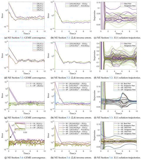
Figure 1. GEME convergence, {2,4}-inverse errors, and trajectories of the ZNN24I model’s $X(t)$ solutions for the NEs in Section 5.1, Section 5.2, Section 5.3 and Section 5.4.

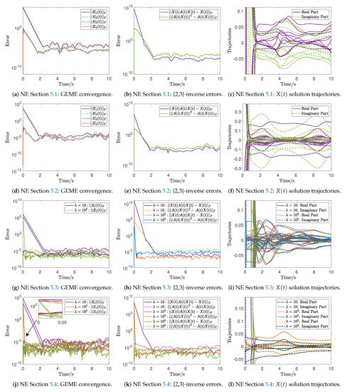
Figure 2. GEME convergence, {2,3}-inverse errors, and trajectories of the ZNN23I model’s $X(t)$ solutions for the NEs in Section 5.1, Section 5.2, Section 5.3 and Section 5.4.

5.2. Numerical Experiment 2

Consider a $10\times 4$ input matrix $A(t)$ of rank 3 with the following real and imaginary parts:

$$\begin{array}{c}B(t)=\left[\begin{array}{cccc}3+\alpha (t)& 3/(t+20)& 5+\beta (2t)& 5+\beta (2t)\\ 2+\alpha (t)& 3+\alpha (2t)& 4-\alpha (t)& 1\end{array}\right],\\ C(t)=\left[\begin{array}{cccc}2\alpha (t)+10& \beta (2t)+3& 4+\alpha (t)& \beta (t)+2\\ 0& 2\alpha (t)+5& 4+\alpha (t)& \alpha (t)+2\end{array}\right],\\ D_{k\times n}(t)={[1+\alpha (t),1+1/2\alpha (t),\cdots ,1+1/k\alpha (t)]}^{\mathrm{T}}\odot {\mathbf{1}}_{k\times n},\\ A_r(t)=\left[\begin{array}{c}B(t)\\ D_{8\times 4}(t)\end{array}\right],A_i(t)=\left[\begin{array}{c}C(t)\\ -{\mathbf{1}}_{8\times 4}-D_{8\times 4}(t)\end{array}\right],\end{array}$$

where ⊙ signifies the Hadamard (or element-wise) product. The results of the ZNN23I and ZNN24I models are depicted in Figure 1d–f and Figure 2d–f, respectively.

5.3. Numerical Experiment 3

Consider a $5\times 4$ input matrix $A(t)$ of rank 3 with the following real and imaginary parts:

$$\begin{array}{c}{A}_r(t)=\left[\begin{array}{cccc}4\alpha (t)+8& 1+\beta (t)& 2t& 2t\\ 6-\alpha (t)& 3/(t+9)& 5-\alpha (t)& 5-\alpha (t)\\ 5/2+\alpha (4t)& 3+t\beta (t)& 2/(t+1)& 2/(t+1)\\ 2\alpha (t)& t\beta (t)-16& 5/2+\alpha (4t)& 5/2+\alpha (4t)\\ 5-\alpha (t)& \alpha (t)+1& 3\beta (t)& 3\beta (t)\end{array}\right],\hfill \\ A_i(t)=-{\mathbf{1}}_{5\times 4}-A_r.\hfill \end{array}$$

The results of the ZNN23I and ZNN24I models are depicted in Figure 1g–i and Figure 2g–i, respectively.

5.4. Numerical Experiment 4

Consider a $3\times 3$ input matrix $A(t)$ of rank 2 with the following real and imaginary parts:

$$\begin{array}{c}{A}_r(t)=\left[\begin{array}{ccc}2+3\alpha (t)& 4+t& 1+2/(t+1)\\ 2+3\alpha (t)& 4+t& 1+2/(t+1)\\ 5-t& \beta (t)& 3\end{array}\right],\hfill \\ A_i(t)=\left[\begin{array}{ccc}2t+10& 2\alpha (t)+3& -2\beta (2t)\\ 2t+10& 2\alpha (t)+3& -2\beta (2t)\\ -t\alpha (t)& 2/(t+1)& 2\alpha (t)-2\end{array}\right].\hfill \end{array}$$

The results of the ZNN23I and ZNN24I models are depicted in Figure 1j–l and Figure 2j–l, respectively.

5.5. Discussion and Analysis of Numerical Experiments

The performance of the ZNN23I and ZNN24I models for computing time-varying {2,3}- and {2,4}-inverses, respectively, is investigated through the NEs in Section 5.1, Section 5.2, Section 5.3, Section 5.4. In the case of the ZNN24I model, the findings for computing a time-varying {2,4}-inverse are presented in Figure 1, while in the case of the ZNN23I model, the findings for computing a time-varying {2,3}-inverse are presented in Figure 2. Particularly, the GEME convergence of the ZNN24I model is depicted in Figure 1a,d,g,j for the NEs is Section 5.1, Section 5.2, Section 5.3, Section 5.4, respectively, and the GEME convergence of the ZNN23I model is depicted in Figures. Figure 2a,d,g,j for the NEs in Section 5.1, Section 5.2, Section 5.3, Section 5.4, respectively. In all these figures, we observe that the GEME convergence begins at $t=0$ in the range $[0,{10}^6]$, but it ends in different periods t depending on the value of $\lambda$. Particularly, in Figure 1a,d,g,j, we observe that the GEME convergence ends before $t=2.5$, with the lowest values in the range $[{10}^{-6},{10}^{-4}]$. In Figure 1d,j and Figure 2d,j, we observe that the GEME convergence ends before $t=2.5$ for $\lambda =10$ and before $t=0.5$ for $\lambda ={10}^2$, with the lowest values in the range $[{10}^{-9},{10}^{-5}]$. In Figure 1j and Figure 2j, we observe that the GEME convergence ends before $t=2.5$ for $\lambda =10$, before $t=0.5$ for $\lambda ={10}^2$, and before $t=0.05$ for $\lambda ={10}^3$, with the lowest values in the range $[{10}^{-9},{10}^{-5}]$. That is, the GEME of the ZNN23I and ZNN24I models begins from a non-optimal initial condition and converges to the zero matrix. It is important to note that the relative error tolerance value defined in ode15s determines the GEME’s lowest values.

Furthermore, the {2,4}-inverse errors of the ZNN24I model are depicted in Figure 1b,e,h,k for the NEs in Section 5.1, Section 5.2, Section 5.3, Section 5.4, respectively, and the {2,3}-inverse errors of the ZNN23I model are depicted in Figure 2b,e,h,k for the NEs in Section 5.1, Section 5.2, Section 5.3, Section 5.4, respectively. In all these figures, we observe that the error begins at $t=0$ in the range $[{10}^3,{10}^{10}]$, but it ends in different periods t depending on the value of $\lambda$, while its lowest values depend on the relative error tolerance value defined in ode15s. In other words, the {2,3}- and {2,4}-inverse errors of the ZNN23I and ZNN24I models exhibit the same convergence tendency as their associated GEMEs. Finally, the $X(t)$ solution trajectories of the ZNN24I model are depicted in Figure 1c,f,i,l for the NEs in Section 5.1, Section 5.2, Section 5.3, Section 5.4, respectively, and the $X(t)$ solution trajectories of the ZNN23I model are depicted in Figure 2c,f,i,l for the NEs in Section 5.1, Section 5.2, Section 5.3, Section 5.4, respectively. In all these figures, we observe that a particular pattern emerges in the {2,3}- and {2,4}-inverse trajectories before $t=2$ for $\lambda =10$, before $t=0.5$ for $\lambda ={10}^2$, and before $t=0.05$ for $\lambda ={10}^3$.

The following is deduced from the NEs of this section. The convergence of the ZNN23I and ZNN24I models begins from a non-optimal initial condition and converges to the zero matrix in a short amount of time. The relative error tolerance value defined in ode15s determines the GEME’s lowest values, while the GEME convergence ending period t depends on the value of $\lambda$. The {2,3}- and {2,4}-inverses errors and the $X(t)$ solution trajectories behave in the same way due to the convergence tendency of the GEMEs. It is also crucial to note that when the value of the design parameter $\lambda$ is higher, the models converge faster and the overall error is lowered even further. In essence, the time-varying {2,3}- and {2,4}-inverses are computed with outstanding and effective performance by the ZNN23I and ZNN24I models, respectively.

6. Conclusions

In this paper, the problem of computing the time-varying {2,3}- and {2,4}-inverses through the ZNN method was investigated. As a consequence, this study proposed and examined two new ZNN models, called ZNN23I and ZNN24I, respectively, for the computation of the time-varying {2,3}- and {2,4}-inverses. Theoretical results as well as three NEs show that the ZNN23I and ZNN24I models are effective for the computation of the time-varying {2,3}- and {2,4}-inverses, respectively.

Some potential study topics are listed below.

1.

Future studies might examine the use of nonlinear activation functions [33,34] to accelerate the convergence speed of the ZNN dynamics.

2.

ZNN designs with terminal convergence [35,36] could be employed to enhance the ZNN23I and ZNN24I models.

3.

Since generalized inverses are crucial to mathematics, and specifically linear algebra, special types of generalized inverses, such as the time-varying {1,3}- and {1,4}-inverses, can be investigated in future works.

References

- Nenchev, D.N.; Konno, A.; Tsujita, T. Chapter 2—Kinematics. In Humanoid Robots; Nenchev, D.N., Konno, A., Tsujita, T., Eds.; Butterworth-Heinemann: Oxford, UK, 2019; pp. 15–82. [Google Scholar] [CrossRef]
- Canuto, E.; Novara, C.; Massotti, L.; Carlucci, D.; Montenegro, C.P. Chapter 9—Orbit and attitude actuators. In Spacecraft Dynamics and Control; Canuto, E., Novara, C., Massotti, L., Carlucci, D., Montenegro, C.P., Eds.; Aerospace Engineering, Butterworth-Heinemann: Oxford, UK, 2018; pp. 463–520. [Google Scholar] [CrossRef]
- Ciubotaru, B.; Staroswiecki, M.; Christophe, C. Fault tolerant control of the Boeing 747 short-period mode using the admissible model matching technique. In Fault Detection, Supervision and Safety of Technical Processes 2006; Zhang, H.Y., Ed.; Elsevier Science Ltd.: Oxford, UK, 2007; pp. 819–824. [Google Scholar] [CrossRef]
- Huang, H.; Fu, D.; Xiao, X.; Ning, Y.; Wang, H.; Jin, L.; Liao, S. Modified Newton integration neural algorithm for dynamic complex-valued matrix pseudoinversion applied to mobile object localization. IEEE Trans. Ind. Inform. 2020, 17, 2432–2442. [Google Scholar] [CrossRef]
- Noroozi, A.; Oveis, A.H.; Hosseini, S.M.; Sebt, M.A. Improved algebraic solution for source localization from TDOA and FDOA measurements. IEEE Wirel. Commun. Lett. 2018, 7, 352–355. [Google Scholar] [CrossRef]
- Dempster, A.G.; Cetin, E. Interference localization for satellite navigation systems. Proc. IEEE 2016, 104, 1318–1326. [Google Scholar] [CrossRef]
- Ben-Israel, A.; Greville, T.N.E. Generalized Inverses: Theory and Applications, 2nd ed.; CMS Books in Mathematics; Springer: New York, NY, USA, 2003. [Google Scholar] [CrossRef]
- Wang, G.; Wei, Y.; Qiao, S.; Lin, P.; Chen, Y. Generalized Inverses: Theory and Computations; Springer: Berlin, Germany, 2018; Volume 53. [Google Scholar]
- Katsikis, V.N.; Pappas, D.; Petralias, A. An improved method for the computation of the Moore–Penrose inverse matrix. Appl. Math. Comput. 2011, 217, 9828–9834. [Google Scholar] [CrossRef]
- Stanimirović, P.S.; Roy, F.; Gupta, D.K.; Srivastava, S. Computing the Moore-Penrose inverse using its error bounds. Appl. Math. Comput. 2020, 371, 124957. [Google Scholar] [CrossRef]
- Zhang, Y.; Ge, S.S. Design and analysis of a general recurrent neural network model for time-varying matrix inversion. IEEE Trans. Neural Netw. 2005, 16, 1477–1490. [Google Scholar] [CrossRef]
- Chai, Y.; Li, H.; Qiao, D.; Qin, S.; Feng, J. A neural network for Moore-Penrose inverse of time-varying complex-valued matrices. Int. J. Comput. Intell. Syst. 2020, 13, 663–671. [Google Scholar] [CrossRef]
- Sun, Z.; Li, F.; Jin, L.; Shi, T.; Liu, K. Noise-tolerant neural algorithm for online solving time-varying full-rank matrix Moore-Penrose inverse problems: A control-theoretic approach. Neurocomputing 2020, 413, 158–172. [Google Scholar] [CrossRef]
- Wu, W.; Zheng, B. Improved recurrent neural networks for solving Moore-Penrose inverse of real-time full-rank matrix. Neurocomputing 2020, 418, 221–231. [Google Scholar] [CrossRef]
- Zhang, Y.; Yang, Y.; Tan, N.; Cai, B. Zhang neural network solving for time-varying full-rank matrix Moore-Penrose inverse. Computing 2011, 92, 97–121. [Google Scholar] [CrossRef]
- Katsikis, V.N.; Stanimirović, P.S.; Mourtas, S.D.; Xiao, L.; Karabasević, D.; Stanujkić, D. Zeroing neural network with fuzzy parameter for computing pseudoinverse of arbitrary matrix. IEEE Trans. Fuzzy Syst. 2022, 30, 3426–3435. [Google Scholar] [CrossRef]
- Kornilova, M.; Kovalnogov, V.; Fedorov, R.; Zamaleev, M.; Katsikis, V.N.; Mourtas, S.D.; Simos, T.E. Zeroing neural network for pseudoinversion of an arbitrary time-varying matrix based on singular value decomposition. Mathematics 2022, 10, 1208. [Google Scholar] [CrossRef]
- Qiao, S.; Wei, Y.; Zhang, X. Computing time-varying ML-weighted pseudoinverse by the Zhang neural networks. Numer. Funct. Anal. Optim. 2020, 41, 1672–1693. [Google Scholar] [CrossRef]
- Qiao, S.; Wang, X.Z.; Wei, Y. Two finite-time convergent Zhang neural network models for time-varying complex matrix Drazin inverse. Linear Algebra Its Appl. 2018, 542, 101–117. [Google Scholar] [CrossRef]
- Wang, X.; Stanimirovic, P.S.; Wei, Y. Complex ZFs for computing time-varying complex outer inverses. Neurocomputing 2018, 275, 983–1001. [Google Scholar] [CrossRef]
- Katsikis, V.N.; Mourtas, S.D.; Stanimirović, P.S.; Zhang, Y. Solving complex-valued time-varying linear matrix equations via QR decomposition with applications to robotic motion tracking and on angle-of-arrival localization. IEEE Trans. Neural Netw. Learn. Syst. 2022, 33, 3415–3424. [Google Scholar] [CrossRef]
- Stanimirović, P.S.; Katsikis, V.N.; Li, S. Hybrid GNN-ZNN models for solving linear matrix equations. Neurocomputing 2018, 316, 124–134. [Google Scholar]
- Dai, J.; Tan, P.; Yang, X.; Xiao, L.; Jia, L.; He, Y. A fuzzy adaptive zeroing neural network with superior finite-time convergence for solving time-variant linear matrix equations. Knowl.-Based Syst. 2022, 242, 108405. [Google Scholar] [CrossRef]
- Xiao, L.; Tan, H.; Dai, J.; Jia, L.; Tang, W. High-order error function designs to compute time-varying linear matrix equations. Inf. Sci. 2021, 576, 173–186. [Google Scholar] [CrossRef]
- Mourtas, S.D.; Katsikis, V.N. Exploiting the Black-Litterman framework through error-correction neural networks. Neurocomputing 2022, 498, 43–58. [Google Scholar] [CrossRef]
- Mourtas, S.D.; Kasimis, C. Exploiting mean-variance portfolio optimization problems through zeroing neural networks. Mathematics 2022, 10, 3079. [Google Scholar] [CrossRef]
- Katsikis, V.N.; Stanimirović, P.S.; Mourtas, S.D.; Li, S.; Cao, X. Generalized inverses: Algorithms and applications. In Mathematics Research Developments; Chapter Towards Higher Order Dynamical Systems; Nova Science Publishers, Inc.: New York, NY, USA, 2021; pp. 207–239. [Google Scholar]
- Katsikis, V.N.; Mourtas, S.D.; Stanimirović, P.S.; Zhang, Y. Continuous-time varying complex QR decomposition via zeroing neural dynamics. Neural Process. Lett. 2021, 53, 3573–3590. [Google Scholar] [CrossRef]
- Kovalnogov, V.N.; Fedorov, R.V.; Generalov, D.A.; Chukalin, A.V.; Katsikis, V.N.; Mourtas, S.D.; Simos, T.E. Portfolio insurance through error-correction neural networks. Mathematics 2022, 10, 3335. [Google Scholar] [CrossRef]
- Stanimirović, P.S.; Cvetković-Ilić, D.S.; Miljković, S.; Miladinović, M. Full-rank representations of {2,4},{2,3}-inverses and successive matrix squaring algorithm. Appl. Math. Comput. 2011, 217, 9358–9367. [Google Scholar]
- Stanimirović, P.S.; Katsikis, V.N.; Pappas, D. Computation of {2,4} and {2,3}-inverses based on rank-one updates. Linear Multilinear Algebra 2018, 66, 147–166. [Google Scholar] [CrossRef]
- Shaini, B. Computing {2,4} and {2,3}-inverses using SVD-like factorizations and QR factorization. Filomat 2016, 30, 403–418. [Google Scholar] [CrossRef]
- Liao, B.; Zhang, Y. From different ZFs to different ZNN models accelerated via Li activation functions to finite-time convergence for time-varying matrix pseudoinversion. Neurocomputing 2014, 133, 512–522. [Google Scholar] [CrossRef]
- Wang, X.Z.; Ma, H.; Stanimirović, P.S. Nonlinearly activated recurrent neural network for computing the Drazin inverse. Neural Process. Lett. 2017, 46, 195. [Google Scholar] [CrossRef]
- Xiao, L. A finite-time convergent neural dynamics for online solution of time-varying linear complex matrix equation. Neurocomputing 2015, 167, 254–259. [Google Scholar] [CrossRef]
- Xiao, L. A nonlinearly-activated neurodynamic model and its finite-time solution to equality-constrained quadratic optimization with nonstationary coefficients. Appl. Soft Comput. 2016, 40, 252–259. [Google Scholar] [CrossRef]
Publisher’s Note: MDPI stays neutral with regard to jurisdictional claims in published maps and institutional affiliations. |
© 2022 by the authors. Licensee MDPI, Basel, Switzerland. This article is an open access article distributed under the terms and conditions of the Creative Commons Attribution (CC BY) license (https://creativecommons.org/licenses/by/4.0/).