Intelligent Prediction of Customer Churn with a Fused Attentional Deep Learning Model

Abstract

In recent years, churn rates in industries such as finance have increased, and the cost of acquiring new users is more than five times the cost of retaining existing users. To improve the intelligent prediction accuracy of customer churn rate, artificial intelligence is gradually used. In this paper, the bidirectional long short-term memory convolutional neural network (BiLSTM-CNN) model is integrated with recurrent neural networks (RNNs) and convolutional neural networks (CNNs) in parallel, which well solves the defective problem that RNNs and CNNs run separately, and it also solves the problem that the output results of a long short-term memory network (LSTM) layer in a densely-connected LSTM-CNN (DLCNN) model will ignore some local information when input to the convolutional layer. In order to explore whether the attention bidirectional long short-term memory convolutional neural network (AttnBLSTM-CNN) model can perform better than BiLSTM-CNN, this paper uses bank data to compare the two models. The experimental results show that the accuracy of the AttnBiLSTM-CNN model is improved by 0.2%, the churn rate is improved by 1.3%, the F1 value is improved by 0.0102, and the AUC value is improved by 0.0103 compared with the BLSTM model. Therefore, introducing the attention mechanism into the BiLSTM-CNN model can further improve the performance of the model. The improvement of the accuracy of the user churn prediction model can warn of the possibility of user churn in advance and take effective measures in advance to prevent user churn and improve the core competitiveness of financial institutions.

1. Introduction

User churn forecasting has attracted a lot of attention in many industries such as banking, telecommunications, insurance companies and gaming and academia [1]. Churn rates have increased in recent years in various industries, including the financial industry, and the cost of acquiring new users is more than five times the cost of retaining existing users [2]. Therefore, building a subscriber churn prediction model, early warning and effective prediction of subscriber churn possibility so that account managers can take effective measures in advance to prevent subscriber churn is the key for banks to improve their core competitiveness [3,4].

Traditional learning models such as logistic regression [5], support vector machines (SVM) [6], decision tree slearning (DTL) [7], random forest (RF) [8] and other models require a lot of manually designed features (hand-crafted features) and the problem of poor simulation results with large amounts of data on the opposite side. The biggest advantage of a recurrent neural network (RNN) model is that it can learn sequence data well [9], but for the actual learning process of the traditional RNN model, with the growth of time nodes and more inputs, it will be difficult to learn the relationship between the preceding and following text, and it will produce the problem of long-term dependence and the phenomenon of gradient disappearance and explosion [10]. In addition to learning the before-and-after correlation information on time series, it is also important to extract the essential features at different levels from the high-dimensional features [11]. In recent years, the convolutional neural network (CNN) model, which is prominent in image recognition and speech, has a good characterization ability, unlike RNN, which focuses more on extracting local features. RNN can learn potential temporal information from temporal data, but it cannot capture important local features, while CNN can learn local features but ignore temporal information. To address these problems, how to combine both RNN and CNN to compensate their respective shortcomings for learning is an effective solution to this problem. Chai, Y and Bian, Y et al. proposed in 2021 the densely connected LSTM with CNN serial integration of DLCNN (densely connected LSTM-CNN (DLCNN) model), which can better take into account the local and temporal feature problems, but the LSTM layer output results in the serial structure ignore some local information when input to the convolutional layer, and they are prone to overfitting when there are more hidden layers in the LSTM module [12].

The introduction of an attention model (AM) in the classification task enables assigning different weights to the data in the model, thus focusing on the information with higher weights based on the weights, and improving the classification results [13]. The experimental results show that compared with the BiLSTM model, the accuracy of the Attn BiLSTM-CNN model is improved by 0.2%, the churn rate is improved by 1.3%, the F1 value is improved by 0.0102, and the AUC value is improved by 0.0103. Therefore, introducing an attention mechanism into a BiLSTM-CNN can further improve the performance of the model. Improvements in the accuracy of user churn prediction models can provide early warning of the possibility of user churn, allowing effective measures to be taken in advance to prevent user churn and enhance the core competitiveness of financial institutions.

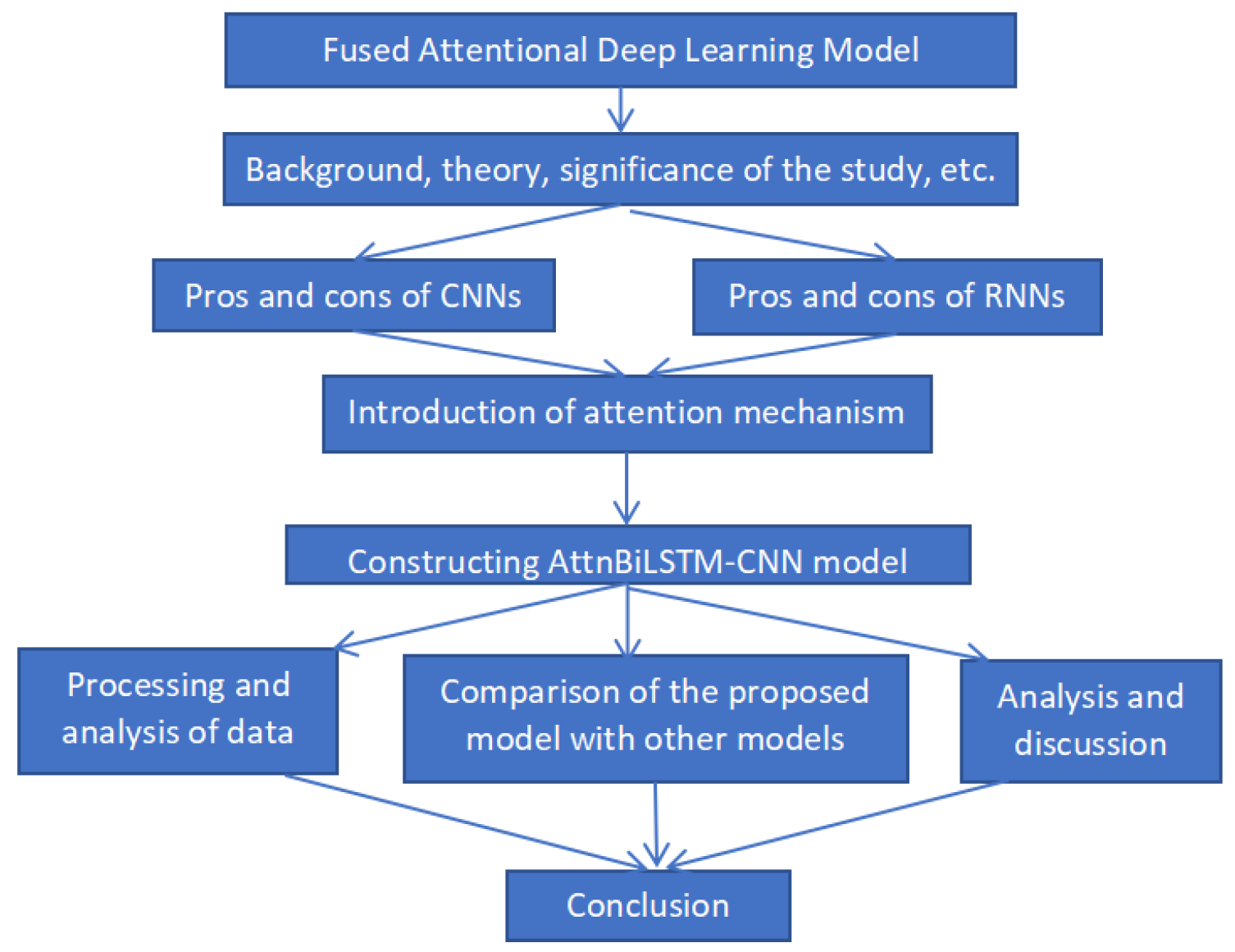
The research in this paper is structured as follows (Figure 1):

• In Section 2, this paper introduces the current status, background and significance of domestic and international research on bank user churn prediction, and it provides a brief review of existing models.
• In Section 3 and Section 4, RNN will have difficulty learning the relationship between the preceding and following texts as the time nodes grow and the inputs increase, and it will suffer from long-term dependency problems and gradient disappearance and explosion. A convolutional neural network has the ability to extract local features and possess good representational power. The serial integration of LSTM and CNN into the DLCNN model can take better care of the problem of local features and temporal features, but in the serial structure, the LSTM layer output results will ignore some local information when input to the convolutional layer, and in the LSTM module, the hidden layers are more prone to overfitting [14].
• In Section 5, since the attention mechanism model can obtain the target area that needs to be focused on, and obtain the target information that it needs to focus on, while suppressing other useless information, it can effectively solve the long-distance dependence problem of neural networks. Therefore, we try to improve the BLSTM-CNN model, introduce the attention mechanism, build the AttnBLSTM-CNN model, and compare the AttnBLSTM-CNN with the BLSTM-CNN to analyze the experimental results.
• In Section 6, the application scheme of the AttnBLSTM-CNN in practical production is presented.

2. Related Work

Traditional learning models such as logistic regression [5], support vector machines (SVM) [6], decision tree slearning (DTL) [7], random forest (RF) [8] and other models require a lot of manually designed features (hand-crafted features) and create the problem of poor simulation results with large amounts of data on the opposite side. In the study of logistic regression models for subscriber churn prediction, Gürsoy used logistic regression and decision tree models with the help of data mining techniques (data mining) to identify subscribers to be churned by the company and create specific advertisements for them using subscriber data from a major telecommunication company in Turkey [5]; Yang, L. et al. proposed a logit leaf model (LLM), a mixture of logistic regression and decision tree, which better solves the problem that decision trees cannot deal with linear relationships and logistic regression cannot solve the problem of interactions between variables. In the study of the support vector machine model in user churn prediction [9]; Kozak, J. and Kania, K. et al. proposed a hybrid method for extracting rules from SVM to be used in Customer Relationship Management (CRM), which solved the problem of poor interpretation of an SVM model [6]. In the study of a decision tree model for user churn prediction, Kozak, J. and Kania, K. et al. used data mining techniques to model the purchase behavior of bank users using the binary classification technique CART classification tree and C5.0 decision tree to simulate user churn, respectively, and the CART classification tree has a high success rate in predicting user churn. Meanwhile, the C5.0 decision tree shows that C5.0 was more effective than the CART classification tree in predicting the success rate of the active class [7]; similarly, Papa, A. and Shemet et al. used data mining techniques to make a decision tree to simulate user churn in a commercial bank [8]. Yang, L. et al. combined under-sampling and SMOTE to better solve the data imbalance problem by using weighted random forest (WRF), which was used to improve the subscriber churn prediction model based on a sample data set in the Indonesian telecommunication industry, and the joint sampling WRF model has better performance compared with the previous prediction models [9]. However, traditional machine models have the problems of requiring a large number of hand-crafted features and poor simulation results in the face of a large amount of data [10].

The biggest advantage of recurrent neural network (RNN) is that it can learn sequence data well [11], because its hidden layer nodes are connected to each other, and the input of the current moment features of the hidden layer contains not only the current moment features but also the previous moment features, so that RNN has “memory capability”. However, in the actual learning process of the traditional RNN model [15], with the growth of time nodes and more inputs, it will be difficult to learn the relationship between the preceding and following text, and it will produce the problem of long-term dependence and the phenomenon of gradient disappearance and explosion [16]. The convolutional neural network (CNN) is prominent in image recognition and speech, unlike the RNN, which focuses more on extracting local features and possesses good representational capability, ignoring temporal information [17]. The BiLSTM and CNN serial integration DLCNN (Densely-connected BiLSTM-CNN (DLCNN) model can take better care of local features and temporal features, but in the serial structure, the output of the BiLSTM layer will ignore some local information when input to the convolutional layer, and it is easy to overfit when there are more hidden layers in the LSTM module [18].

The introduction of an attention model (AM) in the classification task enables assigning different weights to the data in the model, thus focusing on the information with higher weights based on the weights, and improving the classification results [13]. Amornvetchayakul, P et al. introduced the attention mechanism (Attention) in the earliest machine translation in 2014, which has improved the model considerably, and Attention has now become an important concept in the field of neural networks, whose main idea is to obtain the target area that needs to be focused on, to obtain the target information that one needs to focus on, and to suppress other useless information, which can mainly solve the neural network effectively [13]. By introducing Attention on the basis of BiLSTM, the advantages of the Attn-BLSTM-CNN model proposed in this paper are that it effectively solves the problems of losing important features due to the neglect of short-term feature importance and the optimization of long-term temporal pattern mining [12]. The empirical evidence also shows that the CNN-LSTM model with the introduction of the attention mechanism achieves coarse and fine-grained feature fusion, comprehensively portrays the time-series data, and improves the accuracy, which further improves the model’s effectiveness.

3. Construction of the AttnBLSTM-CNN Model

3.1. Overview of CNN Model

The main role of CNN is to extract features from the data. CNN consists of a convolutional layer, pooling layer and fully connected layer. The convolutional layer is the key to extract features, and the convolutional kernels are responsible for extracting the corresponding data features, and the more the number of convolutional kernels, the more abstract the extracted features are. The pooling method is divided into maximum pooling, average pooling, etc. [19]. In this paper, we adopt the maximum pooling method and use the ReLU activation function to ignore some unimportant features, and the ReLU activation function is a segmented linear function with the specific expression as (1) [20]. The fully connected layer serves to expand the neurons after pooling into a one-dimensional vector form, which in turn makes it easier to process the data. However, CNNs have difficulty in learning the relationships between temporal data in prediction, and therefore, enhancements typical of the RNN family of methods are needed to combine CNN methods with LSTM methods.

$$\mathrm{ReLU}=\left\{\begin{array}{cc}x\hfill & x⩾0\hfill \\ 0\hfill & x<0\hfill \end{array}\right.$$

(1)

3.2. The LSTM Model

LSTM is still essentially a recurrent neural network structure of RNN, but it can solve the gradient disappearance problem in RNN because it has a uniquely designed “gate” structure (input gate, forgetting gate and output gate), as shown in Figure 2 [21].

The traditional LSTM network can only learn in one direction, and it cannot obtain the information of the influence from behind to the front, thus causing the partial lack of overall information. In BiLSTM, the input at the current moment depends not only on the information learned before but also on the information learned after, and the two units are combined with each other to fully consider the temporal information before and after. The model structure is shown in Figure 3, and the expression is shown in Equations (2)–(6): where ${\omega }_i(1,\dots ,6)$ denote the weights from one cell layer to another, ${\chi }_i$ denotes the extracted deep feature vector, and $h_t$ denotes the $\{\dots ,{\chi }_{t-1},{\chi }_t,{\chi }_{t+1},\dots \}$, which is the front-to-back input feature sequence forming the LSTM cell, and $h_t^{\prime }$ denotes the $\{\dots ,{\chi }_{t-1},{\chi }_t,{\chi }_{t+1},\dots \}$, which is the LSTM cell composed of feature sequences input from backward to forward, and $O_t$ denotes the output corresponding to the feature vector after passing through the BiLSTM network [22].

$$h_t=\mathrm{sigmoid}(w_1{x}_t+w_2{h}_{t-1}+b^{\left(1\right)})$$

(2)

$$h_t^{\prime }=\mathrm{sigmoid}(w_3{x}_t+w_5{h}_{t+1}^{\prime }+b_t^{\left(2\right)})$$

(3)

$$O_t^{\prime }=\tanh (w_4{h}_t+b_t^{\left(3\right)})$$

(4)

$$O_t^{″}=\tanh (w_6{h}_t^{\prime }+b_t^{\left(4\right)})$$

(5)

$$O_t=\frac{O_t^{\prime }+O_t^{″}}{2}$$

(6)

In Equations (2)–(6), $b_t^{\left(1\right)}$, $b_t^{\left(2\right)}$, $b_t^{\left(3\right)}$, $b_t^{\left(4\right)}$ denotes the bias of the t-th feature vector in the hidden cell in the BiLSTM network. $O_t^{\prime }$ and $O_t^{″}$ are the feature vector output results of the two LSTM units processing the hidden layer information separately at the corresponding moments. In the equation, the feature vector $O_t$ values are the sum of the feature vectors at the two moments and go to the average. Compared with the traditional one-way propagation LSTM, the BiLSTM network can be propagated backward and forward to learn the past information while studying future information, which can obtain more robust temporal information features and is more suitable for the model with more hidden layers [23].

The models BLSTM and CNN each have their advantages but also their limitations. The former can learn potential temporal information from temporal data but cannot capture important local features, while the latter can learn local features but ignore temporal information. To address these problems, in recent years, how to combine both BLSTM and CNN to compensate their respective shortcomings for learning is a better model optimization scheme.

In this paper, the CNN module and the BLSTM module are combined in a parallel manner to form a DLCNN model as shown in Figure 4 of the BiLSTM-CNN structure to avoid the feature loss when the features pass through the BLSTM, and the feature-RNN model is used as an independent input to the CNN module to further increase the feature input to the model. The internal parameter settings of the CNN module are the same as those of the model CNNs, and the internal parameter settings of the BLSTM module are the same as those of the BLSTMs model [24].

3.3. Construction of DLCNN Loss-of-Flow Model

In order to verify the performance of the integrated model DLCNN with the pre-integrated model BLSTMs, the LSTM module in the native DLCNN was replaced with a BLSTM network to form a DLCNN (densely connected LSTM-CNN, DLCNN) model, whose structure before the change is shown in Figure 5a and after the change is shown in Figure 5b.

As shown in Figure 5a, the DLCNN network integrates the RNN network with the CNN network in a serial structure to compensate for the shortcomings of each [25]. The LSTM layer of the original DLCNN is an LSTM network. The LSTM layer of the original DLCNN is an LSTM network. The LSTM module of the original DLCNN was replaced by a BLSTM network. Note that for the convenience of naming the model in the subsequent work, the DLCNN is the improved DLCNN. The structure is illustrated in Figure 5b. In the DLCNN, the input features are Feature_RNN, and the number of hidden units in both the first and second BLSTM layers is 50; the kernel size, number of convolutional kernels, step size and pooling layer parameters of the three convolutional layers are set in the same way as those of the CNNs.

The DLCNN integrates the CNN layers with the BLSTM layers in a serial manner, which compensates for the deficiencies of the BLSTMs and RNNs, but it also has the disadvantage that some local information is ignored when the output of the BLSTM layers is fed to the convolutional layers, which may lead to poor simulation results [26]. To solve this problem, the BLSTMs and CNNs are proposed to be integrated in a parallel way, called BLSTM-CNN, in which Feature_RNN is used as input to the BLSTMs module and Feature_CNN is used as input to the CNNs module, avoiding the loss of information. The BLSTM-CNN model structure is shown in Figure 6.

3.4. Attention Mechanism

The attention mechanism is a resource allocation mechanism that mimics the attention of the human brain. The human brain will focus its attention on the regions that need to be focused at a particular moment, reduce or even ignore attention to other regions to obtain more detailed information that needs to be focused, suppress other useless information, ignore irrelevant information and amplify the desired information [27]. The attention mechanism gives enough attention to the key information by probabilistic assignment to highlight the impact of important information, thus improving the accuracy of the model. The attention mechanism can effectively improve the situation that the LSTM loses information due to long sequences, while replacing the original method of randomly assigning weights by assigning probabilities.

In this paper, the convolutional block attention module (CBAM) is used to implement the attention mechanism. CBAM represents the attention mechanism module of the convolutional module, which is a kind of attention mechanism designed for convolutional neural networks [28].

The simple and effective attention module, which combines spatial and channel attention modules, can achieve better results with an additional spatial ATTENTION compared to SENet. CBAM gives the model the ability to value key features and ignore useless features. CBAM is a lightweight general-purpose module that can be incorporated into various convolutional neural networks for end-to-end training. Its expression is shown in Equation (7).

$$\begin{array}{cc}\hfill M_c\left(F\right)& =\sigma \left(\mathrm{MLP}\right(\mathrm{AvgPool}\left(F\right))+\mathrm{MLP}(\mathrm{MaxPool}\left(F\right)\left)\right)\hfill \\ \hfill & =\sigma \left(W_1\left(W_0\left(F_{\mathrm{avg}}^c\right)\right)\right)+W_1\left(W_0\left(F_{max}^c\right)\right)\hfill \end{array}$$

(7)

Among Equation (7) them, $W_0\in R^{c/r\times c}$. $W_1\in r^{c/r\times c}$.

The spatial attention module focuses on which location information is meaningful and is complementary to the channel attention. Its expression is shown in Equations (8) and (9).

$$M_c\left(F\right)=\sigma \left(f^{7\times 7}\left(\left[\mathrm{AvgPool}\left(F\right)\right]\right)\right)$$

(8)

$$\mathrm{MLP}\left(\mathrm{MaxPool}\left(F\right)\right)=\sigma \left(f^{7\times 7}\left[F_{\mathrm{avg}}^s,F_{max}^s\right]\right)$$

(9)

3.5. AttnBiLSTM-CNN Model

The AttnBiLSTM-CNN model is only changed in the part after the BiLSTM-CNN, while the other modules remain unchanged, so the parts that have been changed will be highlighted, as shown in Figure 7. Figure 8 shows the location of the Attention layer in the AttnBiLSTM-CNN model and its structure, with the Attention layer and the BLSTM layer together called the Attn BLSTM module. The details of the Attention section are described below.

As known from the structure diagram, the implementation of the Attention layer is mainly composed by the summation of the weighting and activation functions [29]. The output coding result of the BLSTM layer is used as the input of the Attention layer, which is weighted (Weight), and the weighting method uses the truncated normal distribution function (as defined in Equation (10)) to randomly generate a number in the range of 0–1, after which the tanh function is used to activate (as defined in Equation (11)), and the summation is performed with softmax to obtain the result of the Attention mechanism. The results are then weighted with the coding results of BLSTM, finally summed, and then decoded to 200 neurons, after the fully connected Dense layer ($\mathrm{utils}=50$), to obtain the output of the Attn BLSTM module.

$$f(x;\mu ,\delta ,a,b)=\frac{\frac{1}{\delta }\mathsf{\Psi }\frac{x-\mu }{\delta }}{\varphi \left(\frac{b-\mu }{\delta }\right)-\varphi \left(\frac{a-\mu }{\delta }\right)}$$

(10)

Here, $X\sim N(\mu ,{\delta }^2)$ when $X\in (a,b)$. $-\infty ⩽a⩽b⩽\infty$ is the probability distribution of X where $\mathsf{\Psi }\left(\epsilon \right)$ is the standard normal distribution and $\mathsf{\Psi }\left(x\right)$ is the cumulative distribution function of the standard normal distribution,

$$\mathrm{tanx}=\frac{e^x-e^{-x}}{e^x+e^{-x}}$$

(11)

4. Data Source and Processing and Model Discriminant

4.1. Data Sources

The original data in this paper come from the user logs, historical deposit and loan and credit data of a city commercial bank, and Figure 9 shows the acquisition process of the original data.

Users’ log data and basic information data are mainly stored in the Oracle database of the bank’s big data platform, which are mapped to the data warehouse Impala through relationships, and then, data mining work is performed through correlation analysis, clustering analysis, regression analysis, and classification, and finally, the original data table is obtained [30]. Pre-processing, feature construction and data balancing are performed on the raw data to obtain the feature data samples suitable for model input.

4.2. Model Discriminant

In the binary classification problem, the samples can be classified according to the combination of their true class and the learner’s predicted class true positive, false positive, true negative and false negative, and we let TP, FP, TN and FN denote their corresponding sample numbers, respectively, we have $\mathrm{TP}+\mathrm{FP}+\mathrm{TN}+\mathrm{FN}=\mathrm{total}$ number of samples. The “confusion matrix” of the classification results is shown in

Table 1. Confusion matrix of classification results.

The Real Situation	Predicted Results
	Positive Example	Counter Example
Positive example	TP (real example)	FN (false counterexample)
Counterexample	FP (false positive Example)	TN (true counterexample)

.

In order to evaluate the performance of different classifiers in user churn prediction, the accuracy is calculated based on the confusion matrix (accuracy), precision (accuracy), recall (recall), and F1-score (F1-score). Accuracy is the ratio of the sum of correctly predicted positive cases to correctly predicted negative cases to the total sample, as shown in Equation (12):

$$\mathrm{accuracy}=\frac{\mathrm{TP}+\mathrm{TN}}{\mathrm{TP}+\mathrm{FN}+\mathrm{FP}+\mathrm{TN}}.$$

(12)

Accuracy is the proportion of positive cases correctly predicted to the sample of positive cases, as shown in Equation (13):

$$\mathrm{precision}=\frac{\mathrm{TP}}{\mathrm{TP}+\mathrm{FP}}.$$

(13)

The detection rate, which indicates how many positive cases in the sample were correctly predicted, i.e., the coverage of positive cases that were predicted, is shown in Equation (14):

$$\mathrm{recall}=\frac{\mathrm{TP}}{\mathrm{TP}+\mathrm{FN}}.$$

(14)

Sometimes, accuracy or completeness cannot describe the efficiency of the classifier alone, where a good performance of one of the indices does not necessarily imply a good performance of another index. For this reason, the F1 value is often used as a metric to evaluate the performance of a classifier, with a closer F1 value to 1 indicating that the model has good combination accuracy and a check-all rate. The F1 value is expressed in Equation (15):

$$\mathrm{F}1=2\times \frac{\mathrm{precision}\times \mathrm{recall}}{\mathrm{precision}+\mathrm{recall}}.$$

(15)

In addition to the above four common evaluation metrics, the ROC curve and the AUC value are used to evaluate the performance of each model. The AUC value is the area obtained by integrating the ROC curve, and the closer the AUC value is to 1, the better the performance of the model.

5. AttnBiLSTM-CNN Experimental Scheme Design

In this paper, AttnBiLSTM-CNN is compared with the BiLSTM-CNN model for experiments to verify the performance of BiLSTM-CNN after introducing Attention. The 104,224 users are divided 7:2:1 into training, validation and test sets. The hardware configuration shown for the experiment includes the CPU (Intel@Xeon@E7-8890, 2.6 Ghz), memory (64 GB), graphics card (Nvidia GTX, 1080 Ti), and hard disk capacity (SSD 1 TB). The experimental software environment configuration includes the operating system (Ubuntu 18.04 64 bit), database (Oracle, hive), programming language (Python 3.7), IDE (Jupyter notebookPycharm) and class libraries (Numpy, pandas, Tensorflow, sklearn matplotlib).

The experiments will evaluate the two methods in terms of precision, completeness, F1 value, ROC curve and AUC value. The results of the experiments are as follows: two models, 50 iterations of each model, and 10,422 users on the test set.

5.1. Accuracy

The best accuracies achieved by AttnBiLSTM-CNN and BiLSTM-CNN in 50 iterations are 95.5% and 95.3%. During the iteration, both Attn BiLSTM-CNN and BiLSTM-CNN accuracies are increasing and slowly stabilize and fluctuate around the optimal accuracy when the optimal accuracy is reached, as shown in Figure 10.

5.2. Rall Rate

The best recall rates achieved by AttnBiLSTM-CNN and BiLSTM-CNN are 97.4% and 96.1% in 50 iterations, respectively. The details are shown in Figure 11.

5.3. F1 Score

The best F1 score obtained by AttnBiLSTM-CNN and BiLSTM-CNN in 50 iterations. The values are 0.958 and 0.952, respectively.The details are shown in Figure 12.

5.4. ROC Curves and AUC Measure

In 50 iterations, the results of the iteration with the highest F1 value for each model were selected and the ROC curves of the two models were plotted; the details are shown in Figure 13. The AUC values of AttnBiLSTM-CNN and BiLSTM-CNN were 0.9678 and 0.9571, respectively.

In 50 iterations, the model with the best F1 value was selected to obtain the accuracy, F1 value and AUC value of each model. The F1 values and AUC values were obtained for each model. The results are shown in

Table 2. Experimental results of AttnBiLSTM-CNN and BiLSTM-CNN.

Model	Metrics
	Precision	Accuracy	Recall	F1	AUC
BLSTM-CNN	0.9531	95.3%	0.9614	0.9521	0.9571
AttnBLSTM-CNN	0.9553	95.5%	0.9743	0.9584	0.9674

The calculation formula can be found in Equations (12)–(15).

.

From the table, it can be seen that among the two models, AttnBiLSTM-CNN and BiLSTM-CNN, the best performing model is AttnBiLSTM-CNN, which achieves 95.53% accuracy and 97.43% completion rate. The F1 value is 0.9584 and the AUC value is 0.9674. It shows that introducing the Attention layer after BLSTM can further improve the performance of the model.

6. AttnBiLSTM-CNN Model Application and Discussion

This section describes the application process of the AttnBiLSTM-CNN model in real production activities, i.e., from data acquisition, data pre-processing, and data feature reconstruction to model training and generation of the churn user table. Figure 14 shows the flow of the application.

The first step needs to complete the mapping from the source database to the data warehouse. Since the actual production source database in the amount of data is very large, in the development, if you do not map to the data warehouse and directly access the source database, it will generate an additional burden on the source database. To affect the development efficiency, it is necessary to carry out the mapping work and develop the tables required to map to the data warehouse. The general mapping work is completed by the database administrator.

After the mapping of data is completed in the second step, the next step is to obtain the data features. This step includes data cleaning, de-duplication, outlier processing and sample equalization, which can be completed directly using SQL scripts.

Then, the third step needs to complete the reconstruction work of the features. The main work is to complete the construction of the two-dimensional feature data into a three-dimensional structure based on the Feature_RNN feature data, with the borrowing method as the division, and obtain the feature data input to the CNN module Feature_CNN.

After obtaining the data file of the model in the fourth step, it is then necessary to call the training code of the model to complete the training of the model and to produce the user churn table file. After the model is trained in the fifth step, the prediction table of user churn is obtained, and

Table 3. Projected results for selected users.

khm	pre_Value	pre	Label	Is_True
1,301,581,754	0.7231	1	1	1
1,119,239,646	0.8232	1	1	1
2,010,363,225	0.3727	0	0	1
1,103,494,309	0.6231	1	1	1
1,303,706,696	0.4823	0	1	0
2,302,096,188	0.4772	0	0	1
1,113,422,243	0.2124	0	0	1
1,301,602,279	0.23215	0	0	1
2,301,502,705	0.8997	1	1	1
1,400,139,233	0.3978	0	0	1
1,302,547,631	0.9231	1	1	1

shows the prediction results for some users.

As shown in Table 3, khm indicates the user number of the user, pre_value indicates the predicted value of the model for the user, pre is the predicted result, 1 indicates that the user is churned, 0 indicates that the user is not churned, label indicates whether the user is actually churned, is_ture indicates whether the user is correctly predicted, and 1 indicates that the prediction is correct. 0 indicates a forecast.

The rapid growth of data is a “double-edged sword”, which brings more management costs to enterprises and also contains more valuable information. The research results of this paper can promote the development of crisis management and early warning theory, establish an artificial intelligence-based customer churn prediction model, predict and warn the churned customers, and save the cost of retaining customers; it can promote the development and application of artificial intelligence. In the face of the huge scale of data and the serious imbalance of data categories, the data are non-linear, not normally distributed and contain noise and other characteristics. Artificial intelligence technology and its improvement techniques can be more effective in processing data with these characteristics.

This paper has conducted an in-depth study of bank user churn prediction, solved a series of problems and obtained a model with a high accuracy rate, which has been applied to a real project.

Financial institutions can use the research results of this paper to achieve precision marketing. By analyzing the data of customers in various dimensions, financial institutions can target marketing to customer preferences, which can greatly save customer acquisition costs and improve customer acquisition efficiency compared with traditional crude distribution. For example, take the specific application scenario of banking business: banks can use their own data (demographic attributes + credit information) + mobile device location information + social housing/consumer information to build a clear user portrait, looking for the target customers who are about to buy a car/housing, to provide financial services (mortgage/consumer loans). After acquiring users, we can predict and reduce the churn rate of stock customers through the user churn model.

7. Conclusions

To improve the accuracy of intelligent prediction of a bank customer churn rate, this paper integrates RNNs (recurrent neural networks) and CNNs (convolutional neural networks) with the BLSTM-CNN (bidirectional long short-term memory) model in parallel, which is a good solution to the problems that come with using RNNs and CNNs. The experimental results show that the accuracy of the Attn BLSTM- CNN model is improved by 0.2%, the churn rate is improved by 1.3%, the F1 value is improved by 0.0102, and the AUC value is improved by 0.0103 compared with the BLSTM model. Therefore, introducing the Attention mechanism into the BLSTM-CNN model can further improve the performance of the model.

From the model perspective, the BLSTM module of AttnBLSTM-CNN has fewer BLSTM layers, and according to the actual business needs, the number of layers can be increased appropriately in this part, which may improve the model. The Attention module is implemented in a simple weighted summation in this paper, and future work will include further exploration of Attention implementation methods. From the perspective of banking business, the current model has the problem of taking up more computing resources in the actual simulation process, and there is still a lot of room for optimization. Another problem is the poor interpretability of the deep learning model; this is a key direction of the current deep learning research. The interpretability of the model can be explored from the point of view of interpretability and help the actual business.