Article

Neural Subspace Learning for Surface Defect Detection

1
School of Mathematics and Information Science, Nanchang Hangkong University, Nanchang 330063, China
2
School of Mathematical Science, Dalian University of Technology, Dalian 116024, China
*
Author to whom correspondence should be addressed.
Mathematics 2022, 10(22), 4351; https://doi.org/10.3390/math10224351
Submission received: 17 October 2022 / Revised: 9 November 2022 / Accepted: 11 November 2022 / Published: 19 November 2022

Abstract

:
Surface defect inspection is a key technique in industrial product assessments. Compared with other visual applications, industrial defect inspection suffers from a small sample problem and a lack of labeled data. Therefore, conventional deep-learning methods depending on huge supervised samples cannot be directly generalized to this task. To deal with the lack of labeled data, unsupervised subspace learning provides more clues for the task of defect inspection. However, conventional subspace learning methods focus on studying the linear subspace structure. In order to explore the nonlinear manifold structure, a novel neural subspace learning algorithm is proposed by substituting linear operators with nonlinear neural networks. The low-rank property of the latent space is approximated by limiting the dimensions of the encoded feature, and the sparse coding property is simulated by quantized autoencoding. To overcome the small sample problem, a novel data augmentation strategy called thin-plate-spline deformation is proposed. Compared with the rigid transformation methods used in previous literature, our strategy could generate more reliable training samples. Experiments on real-world datasets demonstrate that our method achieves state-of-the-art performance compared with unsupervised methods. More importantly, the proposed method is competitive and has a better generalization capability compared with supervised methods based on deep learning techniques.

1. Introduction

Visual inspection is a key step in surface-defect detection of industrial products for ensuring product quality. Compared with manual inspection, automated inspection systems based on computer vision are much more efficient and reliable. A company can save numerous workers by the usage of a vision-based automatic system. In this paper, we focus on the task of product surface defect detection, which is one of the most important steps in industrial manufacturing processes.
The majority of conventional defect detection methods can be summarized in four categories: statistical-based methods [1,2], structural-based methods [3], spectral-based methods [4] and model-based methods [5,6,7,8]. However, most conventional methods are built on hand-crafted visual features and concentrate on studying the linear subspace structure. They suffer from poor generalization and robustness, especially for cases in complex circumstances and variable illumination.
Recently, deep neural networks(DNNs) have demonstrated competitive performance in various fields. They have a powerful ability to extract high-level features. DNNs [9,10,11,12,13,14,15] have also gained great improvements in the task of defect detection compared with traditional methods. Most existing DNN-based inspection methods are based on supervised learning, which implies that a large number of manually annotated data are required. However, the collection of manually annotated data in industrial manufacturing processes is difficult and expensive. Although data augmentation technologies [16,17,18] based on generative adversarial networks (GANs) bring us plausible solutions, the data’s generative ability is limited by the number of samples, especially for the industrial products, whose amounts are only several hundreds or even dozens. Therefore, most existing DNN-based methods still suffer from the small sample problem and a lack of labeled data.
In this paper, a novel unsupervised defect detection method based on neural subspace learning is proposed. The proposed method is created by combining the clear mathematical theory of traditional subspace learning and the powerful learning ability of DNNs. The main assumption of the proposed method is that defect images can be decomposed into two main components: dominant content and sparse flaw regions. This hypothesis is reasonable and common for human-made products and is used in many vision tasks [19,20,21,22]. The dominant background component will be learned by the proposed neural subspace learning method, and the sparse defects will be computed by solving a 1 variational regularization problem.
First, to deal with the lack of labeled data, an unsupervised neural subspace learning method is proposed. The proposed method strives to learn the dominant background component by exploring the latent manifold property of the data in an unsupervised way. Low-rank and sparse representation are two typical manifold structures in subspace learning. Compared with traditional linear subspace learning methods, the proposed method tries to explore the nonlinear subspace structure by integrating traditional low-rank representation theory and sparse coding into a deep autoencoder architecture. In detail, the low-rank property of the latent space is approximated by limiting the dimension of the encoded feature, and the sparse representation property is simulated by a quantized autoencoder.
Second, to deal with the small sample problem, a novel data augmentation strategy called thin-plate-spline deformation is proposed. Due to the fact that most defects to be detected have continuous contours, traditional rigid transformation based augmentation methods will introduce numerous samples in conflict with the ground truth data’s distribution. In contrast, the proposed thin-plate-spline deformation method can generate more reliable training samples by non-rigid spline transformation.
In summary, the main contributions of the proposed method include:
  • A novel, non-rigid data augmentation method is proposed for surface defects detection. The proposed thin-plate-spline deformation method can generate more reliable training samples than rigid transformation based methods.
  • A novel, unsupervised neural subspace learning method is proposed by combining the clear mathematical theory of traditional subspace learning and the powerful learning ability of DNNs.
  • The proposed method achieves competitive performance and has better generalization than other methods.
This paper is organized as follows: Section 2 reviews the existing works of defect detection using supervised and unsupervised methods. In Section 3, we introduce the principle and algorithmic framework of the proposed method in detail. Section 4 contains the implementation details of the proposed algorithm and the experimental results. Conclusions are discussed in Section 5.

2. Related Work

Computer vision has been widely used in defect detection systems. In this section we will briefly review the related work about defect detection, including traditional methods based on hand-crafted features and data-driven deep learning methods.
The majority of traditional approaches can be divided into four categories: statistics-based approaches, structural-based approaches filter-based approaches and model-based approaches [23]. We think these methods are different in extracting high level semantic features consistent with defects, especially the filter-based methods. Statistics-based methods detect defects by computing the spatial distribution of image pixels, such as histogram-of-oriented-gradient [24], co-occurrence matrix [1], and local-binary-pattern [2]. Structural-based approaches mainly focus on the spatial location of textural elements. The main methods are primitive measurement [25], edge features [26], skeleton representation [27] and morphological operations [3]. Filter-based methods employ filter banks to generate features that consist of filter responses. The main methods include spatial domain filtering [28], frequency domain analysis [29] and joint spatial/spatial frequency [4]. Model-based approaches try to obtain certain models with special distributions or attributes, which require a high computational complexity. The main methods include fractal model [5], random field model [6], texem model [7], auto-regressive [8] and the modified PCA model [22]. Especially, the modified PCA model [22] demonstrated that defect-free regions usually had low-rank attributes.
Deep-learning techniques have demonstrated great advantages in the task of defect detection. These works can be classified into supervised learning and unsupervised methods according to whether the annotated data are required.
Supervised learning. Song et al. [9] proposed EDR-Net which utilized the salient object detection method for strip surface defects. Zhang et al. [30] leveraged a real-time surface-defect segmentation network (FDSNet) based on a two-branch architecture to locate the flaw areas. Dong et al. [10] proposed a pyramid feature fusion network with global attention for surface-defect detection. Augustauskas et al. [31] proposed a pixel-level defect segmentation network by using the residual connection and attention gate. Although supervised learning methods obtain pretty good results, a large number of manually annotated data are required. The collection of manually annotated data in industrial manufacturing processes is difficult and expensive. Most existing DNN-based methods suffered from the small sample problem and the lack of labeled data.
Unsupervised learning. Auto-Encoder [32], as a kind of effective and powerful artificial neural network, can learn high-level features by the encoder-decoder architecture. It has been studied for the task of defect detection. Chow et al. [33] trained an auto-encoder on defect-free images and argued that defective pixels would obtain a high reconstructive error. Mujeeb et al. [34] chose binary cross-entropy as a loss function, which measured the distribution error between the reconstructed result and the original data. Tian et al. [35] used cross-patch similarity loss and iteratively chose the best latent variables iteratively. Bergmann et al. [36] proposed the use of a perceptual loss function for examining inter-dependencies among image regions. The loss function was defined to measure the structural similarity by taking into account luminance, contrast, and structural information. In addition, Mei et al. [11] proposed a convolutional denoising auto-encoder network by utilizing multiple Gaussian pyramid features. Similar ideas based on multi-scale features are also used by this literature [37,38]. Yan et al. [39] proposed an adversarial auto-encoder network to monitor defective regions in rolling production. The method combined the power of GAN and the variational auto-encoder, which could be served as a nonlinear dimension reduction technique.
Despite the powerful learning ability of auto-encoder, most existing unsupervised methods did not take into account the prior manifold structure of the data space, such as low-rank and, sparse representation. In this paper, a novel unsupervised defect detection method is proposed by integrating the structure prior to low-rank and sparse representation into the auto-encoder architecture.

3. Methodology

In order to deal with the small sample problem and the lack of labeled data in industrial defect inspection, a novel unsupervised neural subspace learning method is proposed in this section. The pipeline of the proposed method is shown in Figure 1. Firstly, a novel data augmentation method based on non-rigid thin-plate-spline transformation is proposed to deal with the small sample problem. Secondly, a novel auto-encoder regularized by low-rank and sparse representation priors is designed to learn the dominant feature of the image background. Finally, the defects can be detected by solving a 1 variational problem.

3.1. Data Augmentation

Previous researchers usually use rigid transformation, such as flipping, rotating and cropping operations, to augment training datasets. However, due to the fact that most defects in the training data have continuous contours, these rigid operations do not generalize “new” samples. In this paper, a novel data augmentation method based on thin-plate-spline (TPS) deformation method [40] is proposed.
We model the image as a function defined on a 2-dimensional grid X . In order to generate highly reliable samples similar to the true defect images, we first compute a shifted grid Y by shifting each grid point on X through sampling distance in a uniform distribution randomly, then the TPS deformation technique is utilized to fit a smooth warping function between the original grid X and Y to obtain a more realistic twist. In detail, the warping transformation f ( · ) can be computed by solving the following optimization problem
min f X Y f ( X ) 2 + β X f x x + f y y + 2 f x y d x d y ,
where f x x , f x y and f y y denote the second order partial derivatives of warping function f. β is a regularization constant determining the smoothness of the warp. We find that satisfactory results can be obtained when β is randomly generated from the interval [−0.1, 0.1]. Equation (1) can be effectively solved by the method [41].
The augmented training data set is generated through random TPS warping. Figure 2a shows some augmented results by the proposed augmentation method on different kinds of surfaces. It is easy to find that the curve distortions by TPS do not deviate from the defect characteristics in the ground truth training data, and more reliable training samples can be generated by the non-rigid transformation. For example, some new samples of cracked roads are given in the second line of Figure 2a. In contrast, the augmented results (Figure 2b) by rigid transformation are only changed with the variance of view, resolution, etc., and cannot introduce more valuable training data within the same distribution of ground truth data.

3.2. Neural-Subspace Learning with Low-Rank and Sparse Representation Priors

The proposed neural subspace learning method combines the nonlinear learning ability of neural networks and manifold structure priors whose theories and effects have been proved and evaluated in traditional subspace learning [42,43]. By utilizing the priors of manifold structure regularization, such as low-rank and sparse representation, the proposed method can accomplish defect detection in an unsupervised way.
Given the training data X R m × n composed of a collection of defect images X = [ X 1 , X 2 , , X N ] without any annotation, where X i R m is the i-th training sample, m is the dimension of each sample and n is the number of training samples. We assume that X can be decomposed into two components, dominant content and sparse flaw regions. This hypothesis is reasonable and common in many vision tasks [19,20,21,22]. In order to explore the intrinsic manifold structure of the dominant component, low-rank representation is a popular choice [44,45,46] in traditional subspace learning as shown in Equation (2),
min Z , N Z * + λ N 1 , s . t . X = XZ + N
where Z R n × n is self-representation coefficient matrix, N represents the sparse flaw component, λ is a const regularization parameter for adjusting the degree of sparsity, · * denotes the nuclear norm, which is a convex approximation of matrix rank and · 1 defines the sparse elementwise 1 norm.
Although the nuclear norm is an optimal convex approximation of matrix rank, a complex and expensive singular value decomposition operation is required in each iteration. Therefore, another approximation based on the Frobenious norm is proposed [47],
min U , V , N 1 2 ( U F 2 + V F 2 ) + λ N 1 , X = XUV + N
where U R n × d , V R d × n , d n and · F is the Frobenious norm.
In addition to the reduction of optimization complexity, we can learn more from Equation (3). Matrix U and V can be seen as two transformations, i.e., data X is first encoded to a low-dimensional space by X U , then another transformation V maps the latent feature back to the original data space by ( X U ) V . It is interesting to find that the main idea of optimization problem (3) coincides with popular autoencoder, i.e., U and V can be seen as encoder and decoder function. One of the main differences between subspace learning model (3) and deep autoencoder is that traditional subspace learning methods focus on studying linear subspace structure, while autoencoder is designed to learn the nonlinear manifold structure. Despite methods for defect detection ignore the powerful manifold priors used in traditional subspace learning, and they suffer from the small sample problem.
In this section, a novel neural subspace learning framework is proposed by integrating deep autoencoder into the traditional subspace learning method. The proposed neural subspace learning can be represented as follows,
min θ , N 1 2 ( D F 2 + E F 2 ) + λ N 1 , s . t . X = D ( E ( X ) ) + N
where E ( · ) , D ( · ) are respectively the encoder network and decoder network, and θ is the parameters of networks E ( · ) and D ( · ) .
Firstly, the linear transformations U and V in traditional subspace learning are substituted by deep neural networks E ( · ) and D ( · ) . Benefiting from the nonlinear learning potential of neural networks, the proposed method can learn high-level feature representation compared with linear learning methods.
Secondly, in order to make full use of the manifold structure prior, we integrate the deep autoencoder into the traditional learning framework (3). On the one hand, this strategy improves the interpretability of the proposed algorithm. On the other hand, the proposed method can accomplish defect detection in an unsupervised way.
Two kinds of manifold structure priors are utilized in this paper, namely low-rank and sparse representation. As the dominant defect-free surfaces of industrial products are always simple and homologous, low-rank is a proper latent prior. As for encoder and decoder do not have explicit matrix expression, it is hard to optimize 1 2 ( E F 2 + D F 2 ) in Equation (3), we apply two tricks in the designing of a neural network to accomplish the low-rank regularization. The first trick is to implicitly impose a rank constraint on the learned representation by limiting the dimensions of the encoded feature F = E ( X ) to a relatively small constant d n . This implies that the rank of the encoded feature matrix E ( X ) is at most d. The second trick is to remove all nonlinear activation in the decoder to ensure that the rank can not be magnified after a series of linear decode transformations.
Low-rank prior provides a global regularization for the learned feature space. Sparse representation (5) can explore more clues about the local relationship of the image.
min P , α 1 2 F P α 2 + α 1
where P is the overcomplete dictionary, and α is the representation coefficient. In order to integrate the sparse representation prior into the autoencoder, we propose a neural sparse coding framework inspired by the idea of vector quantized variational autoencoder [48]. First, the dictionary P can be simulated by the optimal codebook in VQ-VAE. The learned dictionary P can be regarded as a group on the basis of the latent space extracted by the encoder network. Instead of choosing the nearest code as introduced in reference [48], we propose to learn a sparse representation coefficient vector C s by feeding the encoded feature into a shallow multilayer perceptron (MLP) ϕ as shown in Figure 3, where C s = ϕ ( F ) . To keep the main component learned by VQ-VAE, a regularization loss based on the 1 distance between the learned sparse coefficient C s and the one-hot vector C o learned by VQ-VAE is introduced. The encoded feature F can be reconstructed by a sparse represnetation F ˜ = P C s . Finally, F ˜ will be fed into the decoder network to produce the dominant content by D ( F ˜ ) .
The total loss function for the deep neural-subspace learning method can be summarized as follows,
L ( E ( θ ) , D ( θ ) , P , ϕ , N ) = X D ( P · ϕ ( E ( X ) ) N F 2 + μ C o C s 1 + λ N 1
In summary, the proposed model strives to make full use of the advantage of both subspace learning and neural autoencoder. On the one hand, the method can learn high-level features by utilizing deep neural network. On the other hand, the method can accomplish unsupervised defect detection by integrating low-rank and spare representation priors into the neural network.
The proposed model can be trained by alternate optimization. First, given an initial N , the parameters of the convolutional auto-encoder network and MLP ϕ can be optimized by minimizing
L ( E ( θ ) , D ( θ ) , P , ϕ ) = X D ( P · ϕ ( E ( X ) ) N F 2 + μ C o C s 1
Next, fixing the parameters of all neural networks, the flaw component can be optimized by minimizing
L ( N ) = X D ( P · ϕ ( E ( X ) ) N F 2 + λ N 1
The above optimization problem can be solved analytically by the soft thresholding operator,
( X D ( P · ϕ ( E ( X ) ) ) i , j λ 2 i f ( X D ( P · ϕ ( E ( X ) ) ) i , j > λ 2 ( X D ( P · ϕ ( E ( X ) ) ) i , j + λ 2 i f ( X D ( P · ϕ ( E ( X ) ) ) i , j < λ 2 0 e l s e .
Equations (7) and (8) are alternately optimized until the derivative of the overall objective is below a certain threshold or the maximum iteration number is reached. In the testing phase, given a defect image I , its flawless image can be directly obtained by D ( E ( I ) ) and the noise N can be calculated by Equation (8).

4. Experiments

In this chapter, we will conduct our experiments on two kinds of defect datasets [49,50] and show the results compared with state-of-the-art methods: PCA [51], structural similarity autoencoder (SSIMAE) [36], feature augmented VAE (FAVAE) [38] and encoder-decoder residual network (EDR) [9] and surface-defect segmentation network (FDSNet) [30]. All experiments are implemented using Pytorch and trained on a single Nvidia GeForce RTX 2080ti GPU on Ubuntu 20 system. The learning rate of the Adam optimizer is 0.001 and the constant parameters λ and μ are set to 0.1 and 200, respectively. The training epoch is set to 100 with the batch size set to 64. We follow the rule of taking 80% samples for training and 20% for the test.

4.1. Implement Detail

4.1.1. SD-Saliency-900

SD-Saliency-900 dataset [49] is related to the defect detection of strip steel. In this dataset, we randomly pick 480 images for training and 120 images for testing. For each training image, we use the TPS technique to generate two deformation images. Therefore, we obtain a total of 480 × 3 training images. Before training, we set the initial noise N to zero matrices and its size is equal to the size of the input image. It only costs 6 ms for predicting the corresponding clean image and defect region for a given image.

4.1.2. CrackForest

CrackForest dataset [50] contains 118 defection images of cracked roads. In this dataset, we randomly select 94 images for training and 24 images for testing. First, we transform the original color image into a grayscale image with the size of 128 × 128 . Then, we generate five images for each training image by using the TPS deformation method. In this way, we can expand the original training set by 5 times and obtain 564 training images. In this dataset, the initial noise N is also set to zero matrices. It only takes 6 ms to predict the defect area of a picture.

4.2. Evaluation

We use four quantitative metrics to evaluate the performance of different methods in this paper. They are accuracy, recall, precision and F1-score, respectively, and which are defined by:
A c c u r a c y = T P + T N T P + T N + F P + F N
R e c a l l = T P T P + F N
P r e c i s i o n = T P T P + F P
F 1 = 2 × R e c a l l × P r e c i s i o n R e c a l l + P r e c i s i o n
where true positive (TP) refers to positives that are correctly identified, and true negative (TN) means negatives that are correctly identified. False positive (FP) indicates that negatives still yield positive test results and while false negative (FN) is a test result that falsely indicates that a condition does not hold. Accuracy is the proportion of correct predictions among the total number. Recall measures the proportion of positives that are correctly identified, and Precision is the fraction of relevant instances among the retrieved instances. F1-score that combines precision and recall is the harmonic mean of Precision and Recall.

4.3. Experimental Results

In this section, the method proposed in this paper is first compared with three unsupervised methods by qualitative and quantitative analysis. We also compare the proposed method with two state-of-the-art supervised methods to evaluate the performance and generalization. Finally, an ablation study is conducted to illustrate the advantages of the proposed data augmentation method based on the TPS deformation technique.

4.3.1. Comparison with Unsupervised Methods

Table 1 displays the performance of different defect detection methods on SD-Saliency-900 and CrackForest datasets. It can be found that our method achieves the best results in all of the above four metrics for the SD-Saliency-900 dataset. For another dataset, our method still obtains the best performance in three metrics. For example, compared with PCA, SSIMAE, FAVAE, the F1-score has increased by at least 20 points in the SD-Saliency-900 dataset and almost 30 points in the CrackForest dataset. Although PCA based method get the highest score in the Precision metrics, the Recall metric lags far behind other methods.
Some defect detection samples are displayed in Figure 4 and Figure 5 for different methods on the test datasets of SD-Saliency-900 and CrackForest. For each method, we first separate the original defect image into the clean image and the defect foreground image. Then the defect binary map is obtained by threshold operation. We can find that the FAVAE method detects too many flawless areas because it heavily depends on the thermodynamic map, the detection results of the SSIMAE method contain too much noise due to it is achieved by comparing the similarity of local patches in the image and the PCA method is very suitable for detecting the small defect of the road surface. Compared with these methods, our approach achieves the best detection results.

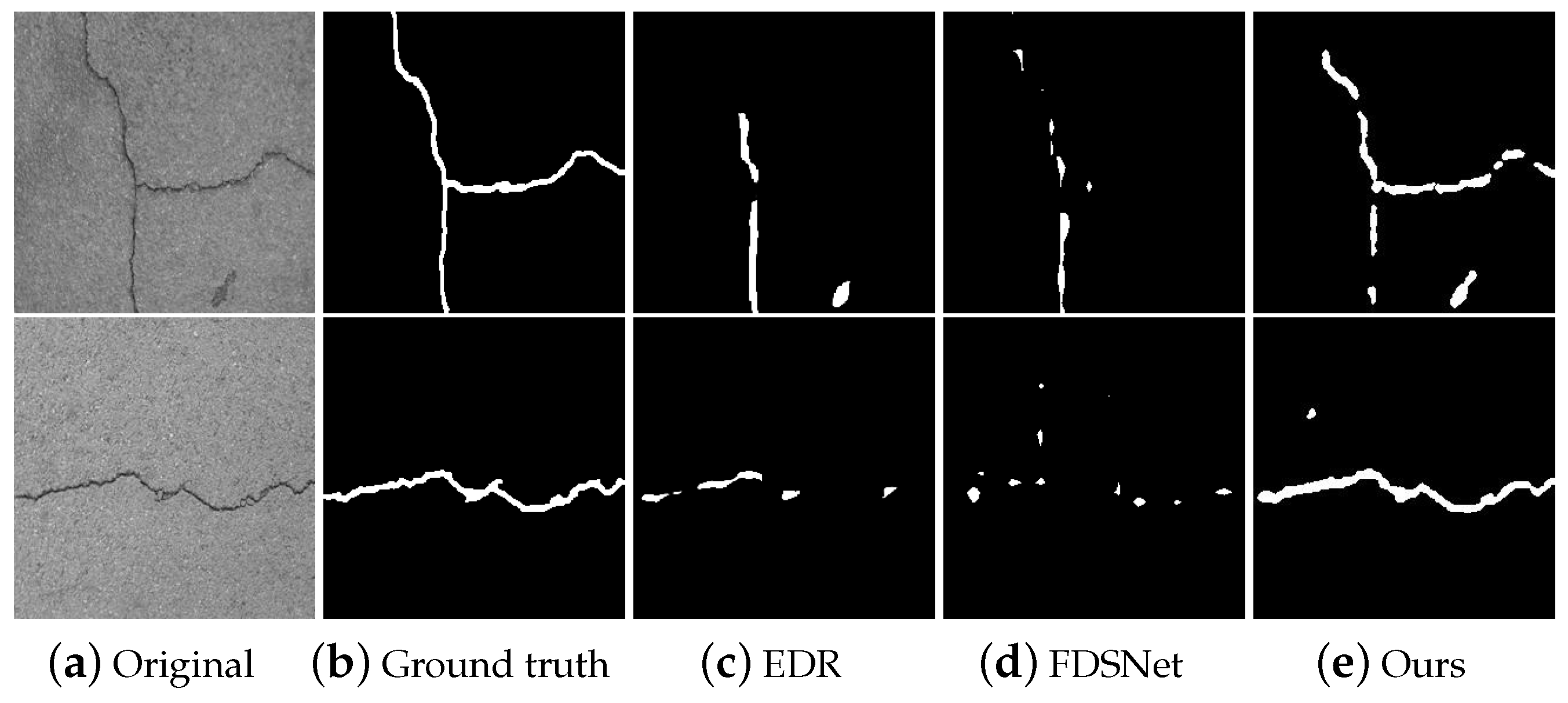
4.3.2. Comparison with Supervised Method

In order to further demonstrate the effectiveness of our unsupervised method, the proposed approach is compared with state-of-the-art defect detection methods, EDR [9] and FDSNet [30]. Both are supervised learning methods. As FDSNet need additional data pre-processing process and they only provide the results of the SD-Saliency-900 dataset, we only compare it to the dataset in the paper. Table 2 shows the results of different methods. Although our methods is weaker than the supervised methods in the SD-Saliency-900 dataset, the proposed method obtains satisfactory results in the CrackForst dataset, especially on the Recall and F1-score metrics, which are important for product quality. These results are acceptable because supervision promotes the network to extract more discriminating features. The visualization results of some test samples are shown in Figure 6 and Figure 7. It can be seen that the detection results of these three methods are very similar. However, supervised learning methods requires a lot of labor to label the data. Our method uses an unsupervised strategy, which is more suitable for industrial production.
In addition, in order to compare the generalization of these methods on a new dataset, we use the cross-domain strategy for testing. Namely, train the model on dataset A and test on datset B. Table 3 gives the quantitative statistical results of EDR method, FDSNet method and ours. It can be found that the EDR and FDSNet methods with supervised learning have very poor performance on the new dataset. As a comparison, our method looks better. Compared with the results without cross-domain test in Table 1, the performance has not dropped much in the precision metric. Figure 8 and Figure 9 show some visualization results by using a cross-domain strategy. From these figures, we can find that the EDR method is completely ineffective in detecting defects. Our method still has good performance.

4.4. Comparison among Different Data Augmentation Strategy

In order to verify the robustness and effectiveness of thin-plate-spline deformation on data augmentation, we conduct some experiments on the SD-Saliency-900 dataset, including training the same network on the dataset without augmentation, with rigid augmentation, with non-rigid augmentation, and with both rigid and non-rigid augmentation, respectively. On the same training dataset, we augment 960, 960 and 1920 images through TPS deformation, rigid transformation and the combination of the above two operations, respectively. The statistical performance of the same test dataset is shown in Table 4. We can find that, the prediction performance of the network which is trained on the dataset without data augmentation falls short. Non-rigid transformation can bring more remarkable performance than rigid operations, such as the Precision and F1-score, and the effectiveness of the combination of two operations is not obvious. Therefore, we do not adopt the combination strategy in this paper.

5. Conclusions

In this paper, a novel unsupervised defect detection method based on neural subspace learning is proposed. The proposed method combines the clear mathematical theory of traditional subspace learning and the powerful learning ability of DNNs. According to the basic assumption that defect images can be decomposed into dominant content and sparse flaw regions, two typical manifold priors, low-rank and sparse representation, are incorporated into the deep neural network. In addition, a new data augmentation method called thin-plate spline deformation is proposed in this paper. Experiments on two datasets demonstrate that the proposed method achieves competitive performance on defect detection tasks.

Author Contributions

Conceptualization, B.L. (Bo Li) and X.L.; Formal analysis, B.L. (Bin Liu) and B.L. (Bo Li); Funding acquisition, B.L. (Bin Liu) and B.L. (Bo Li); Investigation, W.C.; Project administration, B.L. (Bo Li); Resources, B.L. (Bin Liu); Software, W.C.; Supervision, B.L. (Bo Li); Validation, B.L. (Bin Liu), W.C. and B.L. (Bo Li); Visualization, W.C.; Writing—original draft, Weifeng Chen; Writing—review and editing, B.L. (Bin Liu), B.L. (Bo Li) and X.L. All authors have read and agreed to the published version of the manuscript.

Funding

This work was supported in part by Natural Science Foundation of China under Grant (62172198, 61976040, 61762064), Jiangxi Science Fund for Distinguished Young Scholars under Grant (20192BCBL23001), Jiangxi Science and technology project of Education Department under Grant (DA202207128), PHD Start-up Fund of Nanchang Hangkong University (No. EA202107269) and the Opening Project of Nanchang Innovation Institute, Peking University.

Institutional Review Board Statement

Not applicable.

Informed Consent Statement

Not applicable.

Data Availability Statement

SD-Saliency-900: https://github.com/SongGuorong/MCITF/tree/master/SD-saliency-900, accessed on 10 November 2022; CrackForest: https://github.com/cuilimeng/CrackForest-dataset, accessed on 10 November 2022.

Conflicts of Interest

The author declares no conflict of interest.

References

  1. Chen, P.C.; Pavlidis, T. Segmentation by texture using a co-occurrence matrix and a split-and-merge algorithm. Comput. Graph. Image Process. 1979, 10, 172–182. [Google Scholar] [CrossRef]
  2. Guo, Z.; Zhang, L.; Zhang, D. A completed modeling of local binary pattern operator for texture classification. IEEE Trans. Image Process. 2010, 19, 1657–1663. [Google Scholar] [PubMed] [Green Version]
  3. Comer, M.L.; Delp, E.J., III. Morphological operations for color image processing. J. Electron. Imaging 1999, 8, 279–289. [Google Scholar] [CrossRef]
  4. Shapley, R.; Lennie, P. Spatial frequency analysis in the visual system. Annu. Rev. Neurosci. 1985, 8, 547–581. [Google Scholar] [CrossRef] [PubMed]
  5. Majumdar, A.; Bhushan, B. Fractal model of elastic-plastic contact between rough surfaces. J. Tribol. 1991, 113, 1–11. [Google Scholar] [CrossRef]
  6. Bouman, C.A.; Shapiro, M. A multiscale random field model for Bayesian image segmentation. IEEE Trans. Image Process. 1994, 3, 162–177. [Google Scholar] [CrossRef] [Green Version]
  7. Xie, X.; Mirmehdi, M. Texture exemplars for defect detection on random textures. In Proceedings of the International Conference on Pattern Recognition and Image Analysis, Bath, UK, 22–25 August 2005; Springer: Berlin/Heidelberg, Germany, 2005; pp. 404–413. [Google Scholar]
  8. Akaike, H. Fitting autoregressive models for prediction. Ann. Inst. Stat. Math. 1969, 21, 243–247. [Google Scholar] [CrossRef]
  9. Song, G.; Song, K.; Yan, Y. EDRNet: Encoder–decoder residual network for salient object detection of strip steel surface defects. IEEE Trans. Instrum. Meas. 2020, 69, 9709–9719. [Google Scholar] [CrossRef]
  10. Dong, H.; Song, K.; He, Y.; Xu, J.; Yan, Y.; Meng, Q. PGA-Net: Pyramid feature fusion and global context attention network for automated surface defect detection. IEEE Trans. Ind. Inform. 2019, 16, 7448–7458. [Google Scholar] [CrossRef]
  11. Mei, S.; Wang, Y.; Wen, G. Automatic fabric defect detection with a multi-scale convolutional denoising autoencoder network model. Sensors 2018, 18, 1064. [Google Scholar] [CrossRef]
  12. Khalilian, S.; Hallaj, Y.; Balouchestani, A.; Karshenas, H.; Mohammadi, A. PCB Defect Detection Using Denoising Convolutional Autoencoders. In Proceedings of the 2020 International Conference on Machine Vision and Image Processing (MVIP), Qom, Iran, 18–20 February 2020; pp. 1–5. [Google Scholar]
  13. Kang, G.; Gao, S.; Yu, L.; Zhang, D. Deep architecture for high-speed railway insulator surface defect detection: Denoising autoencoder with multitask learning. IEEE Trans. Instrum. Meas. 2018, 68, 2679–2690. [Google Scholar] [CrossRef]
  14. Yu, W.; Zhao, C. Robust monitoring and fault isolation of nonlinear industrial processes using denoising autoencoder and elastic net. IEEE Trans. Control Syst. Technol. 2019, 28, 1083–1091. [Google Scholar] [CrossRef]
  15. Ulutas, T.; Oz, M.A.N.; Mercimek, M.; Kaymakci, O.T. Split-Brain Autoencoder Approach for Surface Defect Detection. In Proceedings of the 2020 International Conference on Electrical, Communication, and Computer Engineering (ICECCE), Istanbul, Turkey, 12–13 June 2020; pp. 1–5. [Google Scholar]
  16. Bird, J.J.; Barnes, C.M.; Manso, L.J.; Ekárt, A.; Faria, D.R. Fruit quality and defect image classification with conditional GAN data augmentation. Sci. Hortic. 2022, 293, 110684. [Google Scholar] [CrossRef]
  17. Chou, Y.C.; Kuo, C.J.; Chen, T.T.; Horng, G.J.; Pai, M.Y.; Wu, M.E.; Lin, Y.C.; Hung, M.H.; Su, W.T.; Chen, Y.C.; et al. Deep-learning-based defective bean inspection with GAN-structured automated labeled data augmentation in coffee industry. Appl. Sci. 2019, 9, 4166. [Google Scholar] [CrossRef] [Green Version]
  18. Wang, C.; Xiao, Z. Lychee surface defect detection based on deep convolutional neural networks with GAN-based data augmentation. Agronomy 2021, 11, 1500. [Google Scholar] [CrossRef]
  19. Zhang, Z.; Ganesh, A.; Xiao, L.; Yi, M. TILT: Transform Invariant Low-rank Textures. In Proceedings of the Asian Conference on Computer Vision, Queenstown, New Zealand, 8–12 November 2010. [Google Scholar]
  20. Peng, Y.; Ganesh, A.; Wright, J.; Xu, W.; Yi, M. RASL: Robust alignment by sparse and low-rank decomposition for linearly correlated images. In Proceedings of the 2010 IEEE Computer Society Conference on Computer Vision and Pattern Recognition, San Francisco, CA, USA, 13–18 June 2010. [Google Scholar]
  21. Candès, E.; Li, X.; Ma, Y.; Wright, J. Robust principal component analysis? J. ACM 2011, 58, 11:1–11:37. [Google Scholar] [CrossRef]
  22. Cao, J.; Wang, N.; Zhang, J.; Wen, Z.; Li, B.; Liu, X. Detection of varied defects in diverse fabric images via modified RPCA with noise term and defect prior. Int. J. Cloth. Sci. Technol. 2016, 28, 516–529. [Google Scholar] [CrossRef]
  23. Czimmermann, T.; Ciuti, G.; Milazzo, M.; Chiurazzi, M.; Roccella, S.; Oddo, C.M.; Dario, P. Visual-based defect detection and classification approaches for industrial applications—A survey. Sensors 2020, 20, 1459. [Google Scholar] [CrossRef] [Green Version]
  24. Niskanen, M.; Silvén, O.; Kauppinen, H. Color and texture based wood inspection with non-supervised clustering. In Proceedings of the Scandinavian Conference on Image Analysis, Bergen, Norway, 11–14 June 2001; pp. 336–342. [Google Scholar]
  25. Kittler, J.; Marik, R.; Mirmehdi, M.; Petrou, M.; Song, J. Detection of Defects in Colour Texture Surfaces. In Proceedings of the MVA, Kawasaki, Japan, 13–15 December 1994; pp. 558–567. [Google Scholar]
  26. Wen, W.; Xia, A. Verifying edges for visual inspection purposes. Pattern Recognit. Lett. 1999, 20, 315–328. [Google Scholar] [CrossRef]
  27. Chen, J.; Jain, A.K. A structural approach to identify defects in textured images. In Proceedings of the 1988 IEEE International Conference on Systems, Man, and Cybernetics, Beijing and Shenyang, China, 8–12 August 1988; Volume 1, pp. 29–32. [Google Scholar]
  28. Odemir, S.; Baykut, A.; Meylani, R.; Erçil, A.; Ertuzun, A. Comparative evaluation of texture analysis algorithms for defect inspection of textile products. In Proceedings of the Fourteenth International Conference on Pattern Recognition (Cat. No. 98EX170), Brisbane, QLD, Australia, 20 August 1998; Volume 2, pp. 1738–1740. [Google Scholar]
  29. Li, X.; Jiang, H.; Yin, G. Detection of surface crack defects on ferrite magnetic tile. NDT E Int. 2014, 62, 6–13. [Google Scholar] [CrossRef]
  30. Zhang, J.; Ding, R.; Ban, M.; Guo, T. FDSNeT: An Accurate Real-Time Surface Defect Segmentation Network. In Proceedings of the ICASSP 2022—2022 IEEE International Conference on Acoustics, Speech and Signal Processing (ICASSP), Singapore, 22–27 May 2022; pp. 3803–3807. [Google Scholar]
  31. Augustauskas, R.; Lipnickas, A. Improved pixel-level pavement-defect segmentation using a deep autoencoder. Sensors 2020, 20, 2557. [Google Scholar] [CrossRef] [PubMed]
  32. Goodfellow, I.; Bengio, Y.; Courville, A.; Bengio, Y. Deep Learning; MIT Press: Cambridge, MA, USA, 2016. [Google Scholar]
  33. Chow, J.K.; Su, Z.; Wu, J.; Tan, P.S.; Mao, X.; Wang, Y.H. Anomaly detection of defects on concrete structures with the convolutional autoencoder. Adv. Eng. Inform. 2020, 45, 101105. [Google Scholar] [CrossRef]
  34. Mujeeb, A.; Dai, W.; Erdt, M.; Sourin, A. One class based feature learning approach for defect detection using deep autoencoders. Adv. Eng. Inform. 2019, 42, 100933. [Google Scholar] [CrossRef]
  35. Tian, H.; Li, F. Autoencoder-based fabric defect detection with cross-patch similarity. In Proceedings of the 2019 16th International Conference on Machine Vision Applications (MVA), Tokyo, Japan, 27–31 May 2019; pp. 1–6. [Google Scholar]
  36. Bergmann, P.; Löwe, S.; Fauser, M.; Sattlegger, D.; Steger, C. Improving unsupervised defect segmentation by applying structural similarity to autoencoders. arXiv 2018, arXiv:1807.02011. [Google Scholar]
  37. Yang, H.; Chen, Y.; Song, K.; Yin, Z. Multiscale feature-clustering-based fully convolutional autoencoder for fast accurate visual inspection of texture surface defects. IEEE Trans. Autom. Sci. Eng. 2019, 16, 1450–1467. [Google Scholar] [CrossRef]
  38. Dehaene, D.; Eline, P. Anomaly localization by modeling perceptual features. arXiv 2020, arXiv:2008.05369. [Google Scholar]
  39. Yan, H.; Yeh, H.M.; Sergin, N. Image-based process monitoring via adversarial autoencoder with applications to rolling defect detection. In Proceedings of the 2019 IEEE 15th International Conference on Automation Science and Engineering (CASE), Vancouver, BC, Canada, 22–26 August 2019; pp. 311–316. [Google Scholar]
  40. Powell, M. A thin plate spline method for mapping curves into curves in two dimensions. In Computational Techniques and Applications: CTAC95; World Scientific: Singapore, 1996; pp. 43–57. [Google Scholar]
  41. Donato, G.; Belongie, S. Approximate Thin Plate Spline Mappings. In Proceedings of the 7th European Conference on Computer Vision-Part III, Copenhagen, Denmark, 28–31 May 2002. [Google Scholar]
  42. Li, B.; Zhao, F.; Su, Z.; Liang, X.; Lai, Y.K.; Rosin, P.L. Example-Based Image Colorization Using Locality Consistent Sparse Representation. IEEE Trans. Image Process. 2017, 26, 5188–5202. [Google Scholar] [CrossRef] [Green Version]
  43. Li, B.; Liu, R.; Cao, J.; Zhang, J.; Lai, Y.K.; Liu, X. Online Low-Rank Representation Learning for Joint Multi-Subspace Recovery and Clustering. IEEE Trans. Image Process. 2018, 27, 335–348. [Google Scholar] [CrossRef] [Green Version]
  44. Liu, G.; Lin, Z.; Yan, S.; Sun, J.; Yu, Y.; Ma, Y. Robust recovery of subspace structures by low-rank representation. IEEE Trans. Pattern Anal. Mach. Intell. 2012, 35, 171–184. [Google Scholar] [CrossRef] [Green Version]
  45. Shi, J.; Yang, W.; Yong, L.; Zheng, X. Low-Rank Representation for Incomplete Data. Math. Probl. Eng. 2014, 2014, 439417. [Google Scholar]
  46. Zhao, Y.Q.; Yang, J. Hyperspectral Image Denoising via Sparse Representation and Low-Rank Constraint. IEEE Trans. Geosci. Remote Sens. 2014, 53, 296–308. [Google Scholar] [CrossRef]
  47. Xiong, L.; Chen, X.; Schneider, J. Direct robust matrix factorizatoin for anomaly detection. In Proceedings of the 2011 IEEE 11th International Conference on Data Mining, Vancouver, BC, Canada, 11–14 December 2011; pp. 844–853. [Google Scholar]
  48. van den Oord, A.; Vinyals, O.; Kavukcuoglu, K. Neural Discrete Representation Learning. In Proceedings of the Advances in Neural Information Processing Systems, Long Beach, CA, USA, 3–9 December 2017; Curran Associates, Inc.: New York, NY, USA, 2017; Volume 30. [Google Scholar]
  49. Song, G.; Song, K.; Yan, Y. Saliency detection for strip steel surface defects using multiple constraints and improved texture features. Opt. Lasers Eng. 2020, 128, 106000. [Google Scholar] [CrossRef]
  50. Cui, L.; Qi, Z.; Chen, Z.; Meng, F.; Shi, Y. Pavement distress detection using random decision forests. In Proceedings of the International Conference on Data Science, Syd, Australia, 8–9 August 2015; Springer: Berlin/Heidelberg, Germany, 2015; pp. 95–102. [Google Scholar]
  51. Abdel-Qader, I.; Pashaie-Rad, S.; Abudayyeh, O.; Yehia, S. PCA-based algorithm for unsupervised bridge crack detection. Adv. Eng. Softw. 2006, 37, 771–778. [Google Scholar] [CrossRef]
Figure 1. Architecture of our low-rank representation quantized network. The sparse result is postprocess with binarization to compare with ground truth. Both encoder E and decoder D contain 4 convolutional layers with size 4 × 4 and step ( 2 , 2 ) . The codebook contains 2000 code and each code is 8 dimensions.
Mathematics 10 04351 g001
Figure 2. Data augmentation based on TPS (a) and rigid transformation (b). The leftmost is the original image for each type of surface, others are deformation results.
Mathematics 10 04351 g002
Figure 3. The pipeline of the learning sparse representation coefficient vector.
Mathematics 10 04351 g003
Figure 4. The results of different approaches on SD-Saliency-900.
Mathematics 10 04351 g004
Figure 5. The results of different approaches on CrackForest.
Mathematics 10 04351 g005
Figure 6. The outputs of EDR method and ours on SD-Saliency-900 dataset.
Mathematics 10 04351 g006
Figure 7. The outputs of EDR method and ours on CrackForest dataset.
Mathematics 10 04351 g007
Figure 8. The results of training on CrackForest and testing on SD-Saliency-900.
Mathematics 10 04351 g008
Figure 9. The results of training on SD-Saliency-900 and testing on CrackForest.
Mathematics 10 04351 g009
Table 1. Quantitative pixel-level defect detection results among unsupervised approaches. The best results are highlighted in bold.
SD-Saliency-900PCASSIMAEFAVAEOurs
Accuracy93.193.687.895.0
Recall14.032.239.041.4
Precision54.657.228.175.8
F1-score22.341.232.653.6
CrackForestPCASSIMAEFAVAEOurs
Accuracy95.195.094.398.5
Recall24.476.260.579.1
Precision80.035.128.171.4
F1-score37.448.138.475.1
Table 2. Quantitative pixel-level defect detection results among different methods.
SD-Saliency-900AccuracyRecallPrecisionF1-Score
EDR95.954.110070.2
FDSNet96.272.972.672.8
Ours95.041.475.853.6
CrackForestAccuracyRecallPrecisionF1-Score
EDR98.256.098.871.5
Ours98.579.171.475.1
Table 3. Quantitative pixel-level defect detection results on cross-domain dataset between EDR and ours. The best results are highlighted by bold fonts.
Train on SD-Saliency-900, Test on CrackForestAccuracyRecallPrecisionF1-Score
EDR91.21.059.21.8
FDSNet97.110.848.917.7
Ours94.334.368.345.7
Train on CrackForest, Test on SD-Saliency-900AccuracyRecallPrecisionF1-Score
EDR97.34.995.99.4
Ours94.77.197.413.2
Table 4. Quantitative pixel-level defect detection results among different augmentation strategies.
SD-Saliency-900AccuracyRecallPrecisionF1-Score
TPS+Rigid95.041.676.053.8
TPS95.041.475.853.6
Rigid93.940.359.548.1
w/o augmentation93.321.555.631.0
Publisher’s Note: MDPI stays neutral with regard to jurisdictional claims in published maps and institutional affiliations.

