Abstract
This work presents a generalized implementation of the infeasible primal-dual interior point method (IPM) achieved by the use of non-Archimedean values, i.e., infinite and infinitesimal numbers. The extended version, called here the non-Archimedean IPM (NA-IPM), is proved to converge in polynomial time to a global optimum and to be able to manage infeasibility and unboundedness transparently, i.e., without considering them as corner cases: by means of a mild embedding (addition of two variables and one constraint), the NA-IPM implicitly and transparently manages their possible presence. Moreover, the new algorithm is able to solve a wider variety of linear and quadratic optimization problems than its standard counterpart. Among them, the lexicographic multi-objective one deserves particular attention, since the NA-IPM overcomes the issues that standard techniques (such as scalarization or preemptive approach) have. To support the theoretical properties of the NA-IPM, the manuscript also shows four linear and quadratic non-Archimedean programming test cases where the effectiveness of the algorithm is verified. This also stresses that the NA-IPM is not just a mere symbolic or theoretical algorithm but actually a concrete numerical tool, paving the way for its use in real-world problems in the near future.
Keywords:
quadratic programming; interior point methods; lexicographic multi-objective optimization; non-standard analysis; infinite/infinitesimal numbers; non-Archimedean scientific computing; fixed-length representations MSC:
90C51; 90C20; 90C29
1. Introduction
Convex quadratic programming (QP) is a widely and deeply studied research topic [1], with plenty of pervasive real-world applications [2]. In spite of the availability of a huge amount of solving algorithms, one of them manifests a pleasant cross-model efficacy at the price of minimal changes in the implementation: the interior point method (IPM) and its variants [3]. Actually, it positively tackles a wide range of optimization tasks, which range from linear programming to cone programming, passing through convex quadratic programming and semidefinite programming.
Another important and of optimization that is growing in interest type is lexicographic multi-objective (linear or nonlinear) programming, which is the task of seeking optimal values of a set of functions (potentially constrained on the domain space) ranked lexicographically (the first objective has priority over the second, the second over the third, and so on [4,5,6,7,8]. Common ways to tackle such a problem are scalarization [9] and preemptive optimization [10] (Chapter 17.7). The scalarization approach transforms the multi-objective problem into a single objective one by computing a weighted sum of the functions according to their priority (the most important one takes a higher weight, the lowest important a lower weight). Unfortunately, the correct a priori choice of the weights is unknown and depends on the function’s range and on the optimal solution as well. The lack of any guarantee of correct convergence is not the only drawback, the choice of too different, i.e., very high and very small weights, may induce a loss of precision and numerical instabilities. On the contrary, a preemptive approach optimizes one function at a time and uses its optimal value as an additional constraint for subsequent tasks. Even if this idea guarantees convergence to optimality, it is not drawbacks-free either. Indeed, it requires solving multiple optimization tasks (one for each function) with increasing complexity (the addition of one constraint after each optimization is completed), which implies wasting computational resources. Furthermore, the nature of the problem can vary and become more complicated over time. For instance, in a QP problem, all the optimizations after the first one shall involve a convex constraint, turning them into quadratically constrained programming problems. As a result, the optimization needs a different, more complex, and less performing algorithm than the one it was supposed to be used at the beginning.
The recent literature has started to reconsider lexicographic problems, trying to solve the issues coming from both scalarization and preemptive approaches leveraging recent developments in numerical non-Archimedean computations [11,12,13]. Some results involve game theory [14,15], evolutionary optimization [16,17,18], and linear programming tackled by Simplex-like methods [4,19,20]. Actually, the key idea is to scalarize the problem by adopting infinite and infinitesimal weights. Such a choice of weights guarantees the satisfaction of lexicographic ordering during the optimization of the single-objective constrained (and non-Archimedean) function. In a nutshell, this idea mixes the good properties of preemptive approaches (guarantee of lexicographic ordering satisfaction and convergence to the problem optimum, if any) and scalarization (transformation of the problem into a scalar one, solving it leveraging common and well-established techniques). Thus, the idea of this work is close to the one presented in [4], but this time using an IPM instead of a Simplex algorithm. Once implemented, the new algorithm, called the NA-IPM (non-Archimedean interior point method) will be able to solve not only lexicographic multi-objective linear programming problems but also quadratic ones, and in a polynomial time. Furthermore, by adding only two variables and one non-Archimedean constraint to the original problem, the NA-IPM is able to handle infeasibility and unboundedness transparently, i.e., without the need to cope with them as corner cases within the implementation. This means that ad hoc routines (such as duality gap norm divergence) or more complex embeddings (e.g., homogeneous self-dual model) can be avoided, preventing possible slowing of computations and the need for different solving algorithms. Lexicographic interpretation apart, the NA-IPM is also able to tackle a huge variety of linear and quadratic non-Archimedean optimization problems as well, as opposed to the non-Archimedean extension of the Simplex algorithm in [4]. Examples of such problems are the non-Archimedean zero-sum games presented in [14].
In line with the recent literature, this work refers to those algorithms (as well as models) as fully implemented (described), leveraging standard analysis with the adjective “standard”. This helps to better distinguish them from their non-Archimedean counterparts which, in the majority of the cases, are built over non-standard models (from here the dichotomy). Actually, this is the case of the NA-IPM, which leverages the non-standard model known as Alpha Theory. Equivalently, one could have used the word “Archimedean” in place of “standard”, but it is far less common and it may have led to misunderstandings. It is also worth stressing that the use of a standard or non-standard approach to model a problem does not imply that the problem itself is inherently standard or non-standard. Rather, the theory within which a problem is modeled just defines the perimeter of tools one can use to tackle it and set a limit to the efficacy of the chosen approach as a consequence. This work proposes a non-standard theory to model some classes of optimization problems and proposes the NA-IPM as a solving approach, believing that there are scenarios where its efficacy is higher than the one of standard techniques.
The remainder of the work is structured as follows: Section 2 and Section 3 provide the basic knowledge to understand this work, the first reviews IPM and the theory behind it, while the second introduces the non-Archimedean model adopted (Benci’s Alpha Theory); Section 4 presents the NA-IPM, discussing algorithm’s theoretical properties (convergence, complexity, etc.), implementation issues, and handling of infeasibility; Section 5 shows four numerical experiments which highlight the NA-IPM’s effectiveness in linear, quadratic, feasible, and infeasible problems. Finally, Section 6 concludes the work with few summarizing lines.
2. Reviewing the Standard Interior Point Method for Quadratic Programming
Quadratic programming (QP) [21] is the task of solving a problem of the form of Equation (1) or Equation (2)
where is the unknown, is symmetric, together with Q forms the cost function, while and are the feasibility constraints, . Whenever Q is also positive semidefinite (), the QP problem can be solved with polynomial complexity [22]; this will be the case study from now on. A very famous algorithm to solve QP problems is the so-called interior point method (IPM) [3], in any of its many fashions: primal/primal-dual, feasible/infeasible, predictor–corrector, or not. The success of IPM has been so wide and great that it pushed [23] to stress its spirit of unification, which has brought together areas of optimization firmly treated as disjoint. Among the reasons for its practical success, one is its astonishing efficiency for very large-scale linear programming problems (where Simplex-like approaches generally get stuck) [24], the capability to exploit any block-matrix structure in the linear algebra operations [25], as well as the possibility to easily and massively parallelize its computations achieving a significant increase in speed (again, the same does not hold for Simplex-like approaches) [25]. Empirical observations add one more positive feature: even if the best implementation of IPM is proved to find an -accurate solution in iterations, in practice it performs much better than that, converging in almost a constant number of steps regardless the problem dimension n [26] ( is the optimality tolerance).
This work focuses on the predictor–corrector infeasible primal-dual IPM [27], which is broadly accepted today to be the most efficient one [3]. The next subsection is devoted to resuming the algorithm in question. The reader already familiar with IPM might find it overly lengthy, but it is better to recall here the details of IPM standard implementation in order to more easily introduce its non-Archimedean extension in Section 4.
Description of the Standard IPM Algorithm
First of all, the assumption that the problem is formulated according to (2) holds. If not, one needs to rewrite the problem by adding some slack variables, one for each constraint, without penalizing them in the cost function. Presolving techniques [28] for guaranteeing consistent problem formulations must be applied too. Second, duality theory [29] states that first-order optimality conditions for QP problems (also known as KKT conditions) are the ones reported in Equation (3), where are the dual variables and s the dual slack variables (a slight modification which includes an additional parameter is provided in Equation (4) and will be discussed later).
Third, iterative algorithms based on the Newton–Raphson method [30] find the solution of systems as the one in (3) (positivity of x and s excluded) starting from a solution and repeatedly solving the linear system in (5) (Equation (6) presents a slight modification with two additional parameters and which will be introduced in the next lines), where and , while X and S are the diagonal matrices obtained by x and s (the iteration apices are omitted for readability reasons).
This system is known as Newton’s step equation, and once solved the approximated solutions of (3) are updated accordingly: with opportunely chosen.
Infeasible primal-dual IPM aims to find optimal primal-dual solutions of (3) by applying a variant of (5) and modifying the search direction as well as the step lengths so that the non-negativity of x and s is strictly satisfied. To do this, the IPM is designed as a path-following algorithm, i.e., an algorithm that tries to stay as close as possible to a specific curve during the optimization [31]. Such a curve, also known as central path, is uniquely identified by all the duality-gap values , where is the primal-dual starting point. Its role is to keep the intermediate solutions away from the feasible region’s boundaries as much as possible (from here we get the word “central”). The points belonging to the central path are those satisfying conditions in Equation (4), which is a slight modification of (3), for a given value of . The uniqueness of the curve is guaranteed whenever the feasible region admits at least one strictly feasible point, that is a primal-dual solution such that (the latter is a very weak assumption). Newton’s step is now computed accordingly with Equation (6), where is the next duality gap to achieve, ; furthermore, uniquely identifies the primal-dual point on the central path to the target. Since Equation (6) approximates (5) more and more closely as goes to zero, if the latter converges to anything as (and it does if the feasible region is bounded), then IPM eventually converges to an optimal solution of the QP problem.
The predictor–corrector version of IPM splits Newton’s direction computation into two stages: predictor and corrector. The predictor one solves the system in (5), i.e., it looks for a solution as optimal as possible, identifying it by the three predictive directions solving Newton’s step equation, namely , , and . Then, it is the turn of the corrector stage, which operates a restoration of some of the centrality lost during the predictor stage. Indeed, pushing all the way towards the optimum may take the temporary solutions too close to the boundaries, affecting the quality of the convergence due to possible numerical issues. To cope with that, the corrector stage solves the linear system in (6) with the constant term (⊙ indicates the Hadamard product). In most cases, the corrector direction badly (but mildly) affects the optimality of the predictor solution, still guaranteeing an improvement with respect to the previous iterate. Indeed, a good centrality of the temporary solutions is too crucial for a good and fast convergence to be ignored. The final optimizing direction is just the sum of the ones found at the two stages. A final remark: since the arbitrary a priori choice of may bias the performance too much, Mehrotra [24] fruitfully proposed an adaptive setting of it to , where .
There are three aspects left to be uncovered to exhaustively present the IPM algorithm used in this work. They consist of three crucial issues of any iterative algorithm: problem infeasibility, starting point choice, and algorithm termination. Multiple ways to address infeasibility exist, two of the most common are iterates divergence [32] and problem embedding [33]. The first one leverages some results on convergence [27], which state that in case of infeasibility the residuals cannot decrease under a positive constant, and, therefore, the iterates must diverge. To identify this phenomenon, it is enough to check at each iteration whether the norm of x and s exceeds a certain threshold , i.e., . On the contrary, the second one aims to embed the given problem in a larger one for which a feasible solution always exists (called an augmented solution). Once found, it tells the user whether the original problem admits a feasible solution (in which case it shall allow one to retrieve it from the augmented one) or the opposite (also specifying which of the polyhedra is infeasible: the primal, the dual, or both).
The starting point choice is vital for the quality of the solution, or even for the convergence itself. In the literature, there exist plenty of papers proposing novel ways to initialize an IPM. In this work, the approach used is the one by Mehrotra [24], which first seeks the solution of the two least squares problems in Equation (7) and (8) in order to satisfy the equality constraints, then executes some additional operations to guarantee strict positivity and well centering (even at the expenses of feasibility). The complete procedure is reported in Algorithm 1.
| Algorithm 1 Starting point computation for IPM. |
Finally, the algorithm termination is demanded to three aggregated values, , , and . They describe the degree of KKT condition (3) satisfaction achieved by the current iteration. As soon as all three values are under a user-defined tolerance threshold , the algorithm is considered converged. Actually, and refer to primal and dual feasibility, respectively, while is in charge of the complementary degree of x and s. Their definition is
A resume of the whole procedure just described can be found in Algorithm 2. The next section introduces the non-Archimedean tools exploited to implement the more general interior point algorithm at the core of this manuscript.
| Algorithm 2 Predictor–corrector infeasible primal-dual IPM. |
|
3. Alpha Theory
This section aims to introduce the non-Archimedean model adopted to generalize the IPM to the NA-IPM: Benci’s Alpha Theory [34]. Its key ingredient is the infinite number , whose definition can be given in multiple ways, as usual in mathematics. In this work, the axiomatization of Alpha Theory given in [12] is used. The reason for this choice is that it provides a very plain and application-oriented introduction to the topic, which also has the property to stress the numerical nature and immediate applicability of such a theory to data science problems. Then, the last part of the section is devoted to showing the strict relation between standard lexicographic QP problems and a particular category of non-Archimedean QP ones. This fact suggests a straightforward application of the NA-IPM to lexicographic problems, as testified by the experimental section.
3.1. Background in Brief
The minimal ground for Alpha Theory consists of three axioms, the first of which introduces a wider field than , namely , which actually contains it.
Axiom 1.
There exists an ordered fieldwhose numbers are called Euclidean numbers.
The second one aims at describing better some of the elements in . Actually, it states that contains numbers that are finite (since it contains ), infinite, and infinitesimal according to the following definition:
Definition 1.
Given , then
- ξ is infinite ⟺
- ξ is finite ⟺
- ξ is infinitesimal
To do this, it introduces the previously mentioned value by means of the numerosity function , which in some sense can be seen as a particular counting function. For the sake of rigorousness, let denote the superstructure on , namely
where ( is the power set)
then set
Axiom 2.
There exists a function, which satisfies
- if A is finite ( denotes the cardinality of a set)
- if
More precisely, Axiom 2 not only introduces the infinite number but also states that its manipulation by means of algebraic functions generates other Euclidean numbers. For instance, the following equivalences hold true in and each one individuates a specific number:
where there is the convention to indicate with , i.e., .
The last axiom introduces the notion of -limit by means of which any function can be extended to a function satisfying all the first-order properties of the former. This is a crucial tool of any non-standard model since it guarantees the transfer of such properties from f to . Because of this, it is commonly referred to as the transfer principle [35].
Axiom 3.
Every sequencehas a unique-limit denoted bywhich satisfies the following properties:
- 1.
- if, then there exists a sequencesuch that
- 2.
- ifthen
- 3.
- ifsuch that, then
- 4.
- any sequence
Leveraging Axiom 3, any real-valued function can be extended to a function by setting [12]
A similar extension is possible for multi-valued functions and sets as well. In the first case, for any with and , is defined as where . In the second case, given a set F, is defined as .
Notice that the use of the word “extension” is fully justified by the fact that . In the remainder of the work, when no ambiguity is possible, the “*” will be omitted, and, therefore, f and will be denoted by the same symbol.
Another important implication of Axioms 1–3 is that any admits the following representation [34]:
where , is a monotonic decreasing function. Finally, we give some definitions which are useful in the remainder of the work.
Definition 2
(Monosemium). is called monosemium if and only if , , .
Definition 3
(Leading monosemium). Given , is called leading monosemium.
Definition 4
(Leading monosemium function). The leading monosemium function is a non-Archimedean function that maps each Euclidean number in its leading monosemium.
Definition 5
(Order of magnitude). The order of magnitude is a function such that .
Definition 6
(Smallest order of magnitude). Let one indicate with the set of Euclidean numbers represented by a limited number of monosemia, i.e., . The smallest order of magnitude is a function such that .
A common generalization of the last two functions to vectorial spaces is the following:
Definition 7
(Infinitesimal number). A way to indicate that is infinitesimal (equivalent to the one in Definition 1) is by the inequality , which is usually indicated as .
3.2. How to Handle Lexicographic Optimization
This subsection aims to introduce Proposition 1, which builds a bridge between standard lexicographic QP problems and non-Archimedean quadratic optimization. First, let one formally introduce standard and non-Archimedean optimization models. Then, the result comes straightforwardly.
Definition 8
(Standard optimization problem). An optimization problem of the form
is said to be standard (or Archimedean) if and only if f, and all and are real-valued multivariate functions.
Definition 9
(Non-Archimedean optimization problem). An optimization problem of the form (11) is said to be non-Archimedean if and only if at least one of the functions f, , or is non-Archimedean, i.e., at least one of them has values in (with ) or maps the input into values in .
Proposition 1.
Consider a lexicographic optimization problem whose objective functions are real functions, and the priority is induced by the natural order. Then, there exists an equivalent scalar program over the same domain, whose objective function is non-standard and has the following form:
where , − 1.
Proof.
The proof will show that the two programs share the same global maxima. Very similar considerations hold for local maxima and global and local minima but are omitted for brevity.
Let Ω be the domain of the two programs, and be a global maximum of the lexicographic optimization problem, i.e., such that , or such that , − 1, and . However, this is true if and only if such that , by the definition of F itself. The latter fact exactly means that ω is a global maximum for the scalar non-standard program. □
The choice of weights adopted in this work is , . As an example, consider the two-objective lexicographic optimization problem in (12). It seeks for the point in the unitary cube which minimizes the first objective . In case more than one such point exists, as in this example where the whole segment optimizes , then such a set of candidate optimal solutions is refined considering the second objective . It is easy to verify that selects as optimal only one point in , namely the origin.
According to Proposition 1, a possible non-Archimedean reformulation of (12) is the one in (13). Here, the objective function is built by summing the first objective weighed by with the second one weighed by , i.e., . Notice that the request holds since . Furthermore, it is clear why the origin also optimizes the second problem. Indeed, as soon as or then assumes positive finite values, while if then assumes positive infinitesimal values. On the other hand, in the origin, it holds , which is a value smaller than any other assumed by the objective function in the previous two cases.
4. Non-Archimedean Interior Point Method
This section aims to introduce a non-Archimedean extension of the predictor–corrector primal-dual infeasible IPM described in Section 2, called by the authors the non-Archimedean IPM (NA-IPM). Such an algorithm is able to solve non-Archimedean quadratic optimization problems and, as a corner case, standard QP ones as well. Three immediate and concrete advantages in leveraging it are: (i) lexicographic QP problems can be solved as they were unprioritized ones (thanks to Proposition 1); (ii) the problem of infeasibility and unboundedness disappears; (iii) more general QP optimization problems can be modeled and solved (Alpha Theory helps in modeling problems that are difficult to model without it, sometimes it is even impossible).
The algorithm pseudocode is presented in Algorithm 3. To better understand it, the next three subsections are devoted to discussing some delicate aspects of it and of its implementation: unboundedness and infeasibility, complexity and convergence properties, and numerical issues that arise when moving from algorithmic description to software implementation. Similarly to what happens for standard algorithms, it is important to stress that many of the proofs in this section assume Euclidean numbers to be represented by finite sequences of monosemia. Indeed, even if the reference set defined by Axioms 1–3 admits numbers represented by infinite sequences, it would not be reasonable to use them in a machine and to discuss the algorithm’s convergence. The reasons are two: (i) the algorithm should manage and manipulate an infinite amount of data; (ii) the machine is finite and cannot store all that information. Notice that, at this stage, the focus is not on variable-length representations of Euclidean numbers, as they would slow the computations down [14]. Fixed-length representations, as the ones discussed in [11] are, therefore, preferred, because they are easier to implement in hardware (i.e., they are more “hardware friendly”), as recent studies testify [36].
| Algorithm 3 Non-Archimedean predictor–corrector infeasible primal-dual IPM. |
|
4.1. Infeasibility and Unboundedness
As stated in Section 2, one can approach the problem of infeasibility and unboundedness in two different ways: divergence detection at run time or problem embedding. While the first keeps the problem complexity fixed but negatively affects the computation because of norm divergence polling, the second wastes resources by optimizing a more complex problem, which is solved efficiently nevertheless. Therefore, the simpler the embedding is, the lesser it affects the performance.
One very simple embedding, proposed by [37,38,39,40], consists of the following mapping:
where and are two positive and sufficiently big constants. This embedding adds two artificial variables (one to the primal and one to the dual problem) and one slack variable (to the primal). The goal of adding the artificial variables is to guarantee the feasibility of their corresponding problem, while on their own dual this is equivalent to adding one bounding hyperplane to prevent any divergence. From duality theory indeed, if the primal problem is infeasible, then the dual is unbounded and vice versa. Geometrically, the hyperplane slope is chosen considering a particular conical combination of the constraints and the constant term vector (the one with all coefficients equal to 1). If there is any polyhedron unboundedness, the conical combination outputs a diverging direction and generates a hyperplane orthogonal to it; otherwise, the addition of such constraints has no effect.
On the other hand, the constraint intercept depends on the penalizing weights and , respectively, for the primal and the dual hyperplane. The larger the weight is, the farther is located the corresponding bound. From the primal perspective instead, and act as penalizing weights for the artificial variables of the dual and the primal problem, respectively. The need for this penalization comes from the fact that to make the optimization consistent, the algorithm must be driven towards feasible points of the original problem, if any. By construction, the latter always have artificial variables equal to zero, which means one has to penalize them in the cost function as much as possible in order to force them to that value. More formally, it can be proved that for sufficiently large values of and : (i) the enlarged problem is strictly feasible and bounded; (ii) any solution for the larger problem is also optimal for the embedded one if and only if both the artificial variables are zero [38].
Unfortunately, this idea is unsustainable when moving from theory to practice, i.e., to implementation. Indeed, a good estimate of the weights is difficult to determine a priori, and the computational performance is sensitive to their values [41]. Trying to find a solution, Lustig [42] investigated the optimal directions generated by Newton’s step equation when and are driven to ∞, proposing a weight-free algorithm based on these directions. Later, Lustig et al. [43] showed that directions coincide with those of an infeasible IPM, without solving the unboundedness issue actually. When considering a set of numbers larger than as , however, an approach in the middle between (14) and the one by Lustig is possible. It consists of the use of infinitely large penalizing weights, i.e., in a non-Archimedean embedding. This choice has the effect of infinitely penalizing the artificial variables, while from a dual perspective it locates the bounding hyperplanes infinitely far from the origin. For instance, in the case of a standard QP problem, it is enough to set both and to , obtaining the following map
The idea to infinitely penalize an artificial variable is not completely new, it has already been successfully used in the I-Big-M method [20], previously proposed by the author of this work, even if in a discrete context rather than in a continuous one.
Nevertheless, there is still a little detail to take care of. Embedding-based approaches leverage the milestone theorem of duality to guarantee optimal the solution’s existence and boundedness. A non-Archimedean version of the duality theorem must hold too, otherwise, non-Archimedean embeddings end up being theoretically not well founded. Thanks to the transfer principle, is free from any issue of this kind, as stated by the next proposition.
Proposition 2
(Non-Archimedean Duality). Given an NA-QP maximization problem, suppose that the primal and dual problems are feasible. Then, if the dual problem has a strictly feasible point, the optimal primal solution set is nonempty and bounded. Vice versa is true as well.
Proof.
The theorem is true thanks to the transfer principle which, roughly speaking, transfers the properties of standard quadratic functions to quadratic non-Archimedean ones. □
If a generic non-Archimedean QP problem is considered instead, setting the weights to may be insufficient to correctly build the embedding. Actually, their proper choice depends on the magnitude of the values constituting the problem. Proposition 3 gives a sufficient estimate of them; before showing it, however, three preliminary results are necessary. Lemmas 1–3 address them. All these three lemmata make use of the functions and provided in Section 3 as Definition 4 and 5, respectively. In particular, Lemma 1 provides an upper bound to the magnitude of the entries of the solutions x of a non-Archimedean linear system . This upper bound is expressed as a function of the magnitude of the entries of both A and b. Furthermore, Lemma 1 considers the case in which the linear system to solve is the dual feasibility constraint of a QP problem, i.e., it has the form with satisfying . Lemmas 2 and 3 generalize Lemma 1 considering corner cases too.
Lemma 1.
Let the set of primal-dual optimal solutions Ω be nonempty and bounded. Additionally, let , A has full row rank, and its entries are represented by at most l monosemia, i.e., . Then, any satisfies
where and .
Proof.
By hypothesis, and, therefore, too. Focusing on the j-th constraint, , it holds
which implies
The proof for the second part of the thesis is very similar:
where is such that and has the form , . Now, following the same guidelines used in (15) and (16), one gets
□
Equation (15) may seem analytically trivial, but actually, it underlines a subtle property of non-Archimedean linear systems: the solution can have entries infinitely larger than any number involved in the system itself. As an example, the 2-by-2 linear system below admits the unique solution . However, each value in the system is finite, i.e., the magnitude of each entry of A and b is :
Notice that Lemma 1 works perfectly here. Indeed, and imply .
Lemma 2.
Let either the primal problem be unbounded or be unbounded in the primal variable. Let also , and A satisfy the same hypothesis as in Lemma 1. Then,
with I and J as in Lemma 1.
Proof.
If the primal problem is unbounded, it means that such that , and such that such that . Nevertheless, a relaxed version of Lemma 1 still holds for the primal polyhedron, that is such that and (the request for optimality is missing). According to (14), a feasible bound for the primal polyhedron is , , provided a suitable choice of . Indeed, it can happen that a wrong value for turns the unbounded problem into an infeasible one. This aspect shall be discussed in Proposition 3, which specifies as a function of .
Choice of apart, the addition of the bound to the primal polyhedron guarantees that such that it is feasible for the bounded primal problem and such that (remember that ξ is the dual variable associated with the new constraint of the primal problem and that ). Following the same reasoning used in Lemma 1, one gets the second part of the thesis
The case in which and unbounded in the primal variable is very similar. Together with the assumption , it means that there are plenty of (not strictly) feasible primal-dual optimal solutions, but there does not exist any with maximum centrality. This fact negatively affects IPMs, since they move towards maximum centrality solutions. Therefore, an IPM that tries to optimize such a problem will never converge to any point, even if there are a lot of optimal candidates. To avoid this phenomenon, it is enough to bound such a set of solutions with the addition of a further constraint to the primal problem (which has also the effect to guarantee the existence of the strictly feasible solutions missing in the dual polyhedron). As a result, the very same considerations applied for problem unboundedness work in this case as well, leading to exactly the result in the thesis of this lemma. □
Lemma 3.
Let either the primal problem be infeasible or be unbounded in the dual variable. Let also , and A satisfy the same hypothesis as in Lemma 1. Then,
with I and J as in Lemma 1.
Proof.
In this case such that but such that . Enlarging the primal problem in accordance to (14), one has that () such that . In addition, it holds such that , provided that for some suitable choice of (which shall be discussed in Proposition 3 as well). By analogous reasoning to the ones used in Lemma 1 and 2, the thesis immediately comes.
The case in which and is unbounded on the dual variable works in the same but symmetric way of the complementary scenario discussed in Lemma 2. Because of this, it implies the bounds stated in the thesis, while the proof is omitted for brevity. □
Proposition 3.
Given an NA-QP problem and its embedding as defined in (14), a sufficient estimate of the penalizing weights is
with I and J as in Lemma 1. In case then , while implies .
Proof.
The extension to the quadratic case of Theorem 2.3 in [38] (proof omitted for brevity) gives the following sufficient condition for and , which holds true even in a non-Archimedean context thanks to the transfer principle:
where (, , ) is an optimal primal-dual solution of the original problem, if any. A possible way to guarantee the satisfaction of Equation (17) is to choose and such that their magnitudes are infinitely higher than the right-hand terms of the inequalities. For instance, one may set
or more weakly
In case Ω is nonempty and bounded, Lemma 1 holds and provides an estimate on the magnitude of both and . In case either the primal problem is unbounded or Ω is unbounded in the primal variable, Lemma 2 applies: the optimal solution is handcrafted by bounding the polyhedron, its magnitude is overestimated by , and (17) gives a clue for a feasible choice of . Similar considerations hold for the case of either primal problem infeasibility or Ω unboundedness in the dual variable, where Lemma 3 is used.
Corner cases are the scenarios where either or . Since implies , the primal problem is either unbounded or with unique feasible (and optimal) point . In both cases, it is enough to set . Since is a feasible solution, in the case of unboundedness it must exist a feasible point with at least one finite entry and no infinite ones because of continuity. In the other scenario, is the optimal solution and, therefore, any finite vector is a suitable upper bound for it. Analogous considerations hold for the case , where a sufficient magnitude bound is . □
4.2. Convergence and Complexity
The main theoretical aspects to investigate in an iterative algorithm are convergence and complexity. Notice that in the case of non-Archimedean algorithms, the complexity of elementary operations (such as the sum) assumes their execution on non-Archimedean numbers, rather than on real ones. Since, theoretically, the NA-IPM is just an IPM able to work with numbers in , one first result on NA-IPM complexity comes straightforwardly thanks to the transfer principle. It is worth stressing that, as usual, Theorem 1 assumes to apply the NA-IPM to an NA-QP problem whose optimal solutions set is non-empty and bounded.
Theorem 1
(NA-IPM convergence). The NA-IPM algorithm converges in , where is the primal space dimension and is the optimality relative tolerance.
Proof.
The theorem holds true because of the transfer principle. □
In spite of this result being remarkable, it is of no practical utility. Indeed, the relative tolerance may not be a finite value but an infinitesimal one, making the time needed to converge infinite. However, under proper assumptions, finite time convergence can also be guaranteed, as stated by Theorem 2. Before showing it, some preliminary results are needed and are presented as lemmas. In fact, Lemma 4 guarantees optimality improvement iteration by iteration, Lemma 5 provides a preliminary result used by Lemma 6 which proves the algorithm convergence on the leading monosemium.
Lemma 4.
In the NA-IPM, if then such that and .
Proof.
Applying the transfer principle to Lemma 6.7 in [27], it holds true that
where C is a positive constant at most finite. Equation (18) immediately implies and . The assumption completes the proof. □
Lemma 5.
Let be the right-hand term in (6) at the k-th iteration, and the vector of its last n entries. If the temporary solution (see Lemma 6 for its definition), then .
Proof.
By definition, . Focusing on the radicand, one has
where the strict inequality comes from the fact that by hypothesis, which implies . Considering again the square root, the result comes straightforwardly:
□
Lemma 6.
Let be the NA-IPM starting point, and be the compact form for Newton’s step Equation (6) at the beginning of the optimization. Let one rewrite the right-hand term , where Call the first entries of and the last n, i.e., . Then, such that and and the Newton–Raphson method reaches that iteration in .
Proof.
As usual, the central path neighborhood is
Lemma 4 and μ’s positivity implies that . The application of the transfer principle to Theorem 6.2 in [27] guarantees that such that holds true and the Newton–Raphson algorithm reaches that iteration in . Together, Lemma 4 and guarantee that (reached in polynomial time as well) such that too. Set . Then, one has and . Moreover, by construction it holds and (the latter comes from Lemma 5). Therefore, the following two chains of inequalities hold true:
as stated in the thesis. □
Corollary 1.
Let k satisfy Lemma 6, then either
Proof.
The result comes straightforwardly from three facts: (i) ; (ii) ; (iii) the leading term of entry of x, s, and λ is never zeroed since the full optimizing step is never taken (see lines 19–20 and 31–32 in Algorithm 2). □
We are now ready to provide the convergence theorem for the NA-IPM.
Theorem 2
(NA-IPM convergence). The NA-IPM converges to the solution of an NA-QP problem in , where is the primal space dimension, is the relative tolerance, and is the number of consecutive monosemia used in the problem optimization.
Proof.
For the sake of simplicity, assume to represent all the Euclidean numbers in the NA-QP problem by means of the same function of powers . From the approximation up to l consecutive monosemia, one can rewrite and . Lemma 6 guarantees that for which is ε-satisfied. Now, update the temporary solution substituting each entry of x and s which satisfies Corollary 1 with any feasible value one order of magnitude smaller, e.g., satisfying Corollary 1 is replaced with a positive value of the order , where is such that . Actually, they are those variables that are not active at the optimal solution, at least considering the zeroing of only. Then, recompute , which by construction satisfies , . All these operations have polynomial complexity and do not affect the overall result. Updating the right-hand term as and zeroing the leading term of those entries whose magnitude is still . Next, algorithm iterations are forced to consider the previous as already fully satisfied. What is actually happening is that the problem now tolerates an infeasibility error whose norm is equal to . Therefore, one can apply Lemma 6 again to obtain one solution which is ε-optimal on the second monosemia of too, and this result is achieved with a finite number of iterations and in polynomial complexity. Repeating the update-optimization procedure for all the l monosemia by means of which is represented, one obtains one ε-optimal solution on all of them. Since each of the lε-satisfactions is achieved in , then the whole algorithm converges in . □
The next proposition highlights a particular property of the NA-IPM when solving lexicographic QP problems. Actually, it happens that every time decreases by one order of magnitude, then one objective is -optimized.
Proposition 4.
Consider an NA-QP problem generated from a standard lexicographic one in accordance with Theorem 1 and . Then, each of the l objectives is ε-optimized in polynomial time and when the i-th one is ε-optimized the magnitude of μ decreases from to in the next iteration.
Proof.
Assume to start the algorithm with a sufficiently good and well-centered solution, as the one produced by Algorithm 1, then, . Since by construction, one can interpret each monosemia in as the satisfaction of the corresponding objective function at the k-th iteration, that is if then the first objective lacks to be fully optimized, the second one lacks , and so on. Because of Lemma 6, in polynomial time, is ε-optimized, that is, the KKT conditions (3) are ε-satisfied. In fact, this means that primal-dual feasibility is close to finite satisfaction and centrality is finitely close to zero. There is a further interpretation nevertheless. Interpreting the KKT conditions from a primal perspective their ε-satisfaction testifies that: (i) the primal solution if feasible (indeed, the primal is a standard polyhedron and, therefore, is enough to consider the leading terms of x only, getting rid of the infinitesimal infeasibility ); (ii) the objective function is finitely ε-optimized (which means that the first objective is ε-optimized since the original problem was a lexicographic one and the high-priority objective is the only one associated with finite values of the non-Archimedean objective function); (iii) the approximated solution is very close to the optimal surface of the first objective, roughly speaking it is ε-finitely close. Moreover, the fact that after the updating procedure used in Theorem implies that the magnitude of μ will be one order of magnitude smaller in the next iteration, i.e., it will decrease from to . Since what was just said holds for all the l monosemia (read priority levels of, i.e., objectives in the lexicographic cost function), the proposition is proved true. □
4.3. Numerical Considerations and Implementation Issues
The whole field cannot be used in practice since it is too big to fit in a machine. However, the algorithmic field presented below is enough to represent and solve many real-world problems:
where is a monotone decreasing function and the term “algorithmic field” refers to finite approximations of theoretical fields realized by computers [12]. Similarly to IEEE-754 floating point numbers, which is the standard encoding for real numbers within a machine, a finite dimension encoding for Euclidean numbers in is needed. In [11,12], the bounded algorithmic number (BAN) representation is presented as a sufficiently flexible and informative encoding to cope with this task. The BAN format is a fixed-length approximation of a Euclidean number. An example of BAN is , where the “precision” in this context is given by the degree of the polynomial in plus 1 (three in this case). The BAN encoding with degree three is indicated as BAN3.
The second detail to take care of when attempting to do numerical computations with Euclidean numbers is the effect of lower-magnitude monosemia on them. For instance, consider a two-objective lexicographic QP whose first objective is degenerate with respect to some entries of x. When solving the problem by means of the NA-IPM, the following phenomenon (which can also be proved theoretically) occurs: the information of the optimizing direction for the secondary objective is stored as an infinitesimal gradient in the solution of Newton’s step Equation (6). As an example, assume that and the entries and are degenerate with respect to the first objective. Then, at each iteration the infinitesimal monosemium in the optimizing direction of assumes a negligible value, while for and this is not true: it is significant and grows exponentially in time. In fact, the infinitesimal gradient represents the optimizing direction which must be followed along the optimal (and degenerate) surface of the first objective in order to also reach optimality for the second one. However, such infinitesimal directions do not significantly contribute to the optimization, since the major role is played by the finite entries of the gradient. Therefore, the effect of this infinitesimal information in the gradient only generates numerical instabilities. As soon as the first objective is -optimized, i.e., the first objective surface is reached, the optimizing direction still assumes finite values but this time oriented in order to optimize the second objective keeping the first one fixed, while all the infinitesimal monosemia of the gradient assume negligible values. Roughly speaking, it happens as a sort of “gradient promotion” as a result of the change in the objective to optimize. To cope with the issue of noisy and unstable infinitesimal entries in the gradient, two details need to be implemented: (i) after the computation of the gradients (both the predictor and the corrector step), only the leading term of each entry must be preserved, zeroing the remaining monosemia; (ii) after having computed the starting point according to Algorithm 1, again only the leading term of each entry of x, s, and must be preserved. These variations do not affect convergence nor the generality of the discussion since the leading terms of the primal-dual solution are the only ones that impact the zeroing of .
The choice of dealing with only the leading terms of the gradients comes in handy to solve another issue during the computations: a good choice for the value to assign to the zeroed entries of x and s during the updating phase discussed in Theorem 2. Actually, it is enough to add one monosemium whose magnitude is such that the following equality holds true: . For instance, assume again a two-objective lexicographic QP scenario after having completed the optimization of the first one. It holds true that and either or are smaller than , say . Then, the updating phase of Theorem 2 sets to a value having magnitude one order smaller. A reasonable approach is to set equal to a monosemium, say , such that . Since is finite because of Corollary 1, one has . The naive choice is , but it may be not the best one. Indeed, this approach does not guarantee the generation of a temporary solution with the highest possible centrality, i.e., , where is the centrality measure after the update. To do it, the value to opt for must be , where and is a monosemium one order of magnitude smaller than and sufficiently (but arbitrarily) far from zero.
Another numerical issue to care about is the computation accuracy due to the number of monosemia used. As a practical example, consider the task to invert the matrix A reported below. Since its entries have magnitudes from to , one may think BAN3 encoding is enough to properly compute an approximation of its inverse, which is reported below as . However, the product testifies the presence of an error whose magnitude is , quite close to . Depending on the application, such noise could negatively affect further computations and the final result. Therefore, a good practice is to foresee some additional slots in the non-Archimedean number encoding. For instance, adopting the BAN5 standard, the approximated inverse manifests an error with magnitude (see matrix ), definitely a safer choice even if at the expense of extra computational effort.
Finally, the last detail concerns terminal conditions. In the standard IPM, execution stops when the three convergence measures , , and in (9) are smaller than the threshold . However, in a non-Archimedean context optimality means to be -optimal on each of the l monosemia in the objective function, i.e., to satisfy the KKT condition (3) on the first l monosemia in b and c and . This means that the terminal condition needs to be modified in order to cope with such a convergence definition. The convergence measures need to be redefined as
with the convention . In this way, one has the guarantee that , , and are finite values when close to optimality. To better clarify this concept, consider the case in which b has only infinitesimal entries. This implies that the norm of b is infinitesimal too. In case the convergence measures in (9) are used, the denominator of is a finite number. Therefore, any finite approximation of b, i.e., any primal solution x such that , is finite induces a finite value for . This is definitely a bad behavior since it is natural to expect that: (i) the convergence measures are finite numbers only if the optimization is close to optimality; (ii) their leading monosemium is smaller than when the leading monosemium of the residual norm ( in this case) is small as well. However, this is not the case in the current example as assumes finite values for approximation errors of b which are infinitely larger than its norm. Using the definitions in (19) instead, the issue is solved since now finite approximations of b are mapped into infinite values of , while infinitesimal errors are mapped into finite ones. In fact, the introduction of the magnitude of the constant term vectors in the definitions avoids the bias which would have been introduced by an a priori choice of the magnitude of the constant term added to the denominator of the convergence measures.
Then, feasibility on the primal problem is -achieved when the absolute value of the first monosemia in are smaller than , i.e., assuming and , a sufficient level of optimality is reached when , . Similar considerations hold for c and as well.
5. Numerical Experiments
This section presents four problems by means of which the efficacy of the NA-IPM is tested. The first, the third, and the fourth are lexicographic ones, while the second involves non-Archimedean numbers also in the constant term b. They are listed in increasing order of difficulty, from LP to QP problems, from two to three objective functions, passing through unboundedness tackling. In all the experiments, is set to , a de facto standard choice.
5.1. Experiment 1: Two-Objective LP
The first experiment uses a benchmark already exploited to evaluate the efficacy of non-Archimedean optimizers [4,20]. In [4], for instance, the algorithm used was a non-Archimedean version of the Simplex method, able to deal with non-Archimedean cost functions and standard constraints. On the contrary, here the adopted algorithm is a non-Archimedean generalization of the primal-dual IPM, which is intrinsically implemented to cope with non-Archimedean functions both at the level of cost function and constraints. Another difference is the fact that Simplex-like algorithms are discrete ones, while IPMs are continuous procedures.
The problem formulation is in Equation (20). Geometrically, the first and most important objective identifies as optimal the whole segment linking the point to , highlighted in red in Figure 1. When considering also the second objective , only one point of this segment turns out to be truly optimal: the vertex . A red star indicates it in Figure 2. Equation (21) reports the non-Archimedean representation of the problem: the two objectives are scalarized into one single cost function by a weighting sum: the first one is left as is while the second is scaled down by the factor , testifying to the precedence (read importance) relation between the two (recall from Section 3 that is an infinitesimal value, defined as the reciprocal of ).
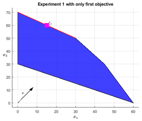
Figure 1.
The optimal segment for the primary objective is in red; is the optimal point a standard IPM would approach.
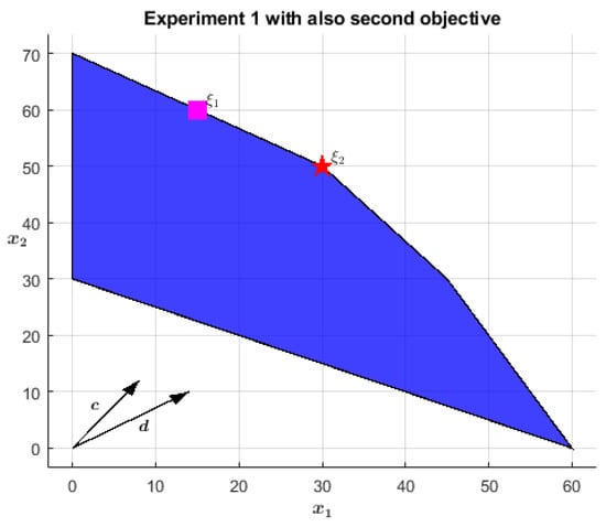
Figure 2.
is the only optimal solution when both objectives are considered.
As already stressed, any IPM favors solutions with higher centrality and the NA-IPM is not an exception. This aspect becomes particularly evident in the case of multiple optimal solutions since the optimizing algorithm converges to the analytic center of the optimal surface. Proposition 4 implicitly states that in lexicographic problems the NA-IPM primarily optimizes the first objective, then the second one, and so on. Since in (20) the optimal region for the first objective is a segment, in the first place the NA-IPM moves towards its midpoint , marked by a magenta square in Figure 1. Eventually, the first cost function is -optimized and the secondary objective starts to mainly condition the optimization, moving the temporary solution towards until termination conditions are satisfied. This change in leadership is testified when the centrality measure turns from finite to infinitesimal, as discussed in Theorem 2, Proposition 4, and Section 4.3. With reference to Table 1, one can appreciate this phenomenon between lines 5 and 6. At line 5, the current solution is very close to , actually , while has assumed for the last time a (very small) finite value. These facts testify that the first objective is -satisfied, therefore, in the next step, the algorithm will move towards and show an infinitesimal centrality measure, as confirmed by line 6 where the target point is . Moreover, the improvement in the objective function from step 5 to step 6 is infinitesimal, which further stresses that the algorithm has already reached the first objective -satisfaction and it is moving along its degenerate surface. Similar numerical confirmations come from the other experiments and are highlighted in boldface in the associated tables.

Table 1.
Iterations of the NA-IPM solving the problem in (20).
5.2. Experiment 2: Unbounded Problem
The second experiment aims to numerically show the efficacy of the mild embedding shown in Section 4.1 to cope with infeasibility and unboundedness. As an example, consider the 2D unbounded problem described in Equation (22) and drawn in Figure 3, which is already analytically reported in normal form as in (2) for the sake of clarity. To mitigate the issues coming from the iterates divergence, one can resort to the embedding described in Equation (14), obtaining the strictly feasible and bounded problem in (23). Proposition 3 recommends the use of penalizing weights such that ; the choice has been .
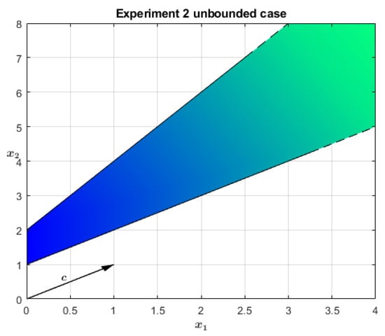
Figure 3.
Example of an unbounded primal polyhedron.
Table 2 reports the iterations made by the NA-IPM to solve such an extended problem. As expected, the algorithm converges in a finite number of steps, and the optimal point lies on the bounding hyperplane located infinitely far from the origin. Formally, what gives a clue about the unboundedness of the problem is the dual variable , see Proposition 3. If the problem is bounded then it must be zero in the optimal solution, while it is equal to 1. In this specific case, however, there is another and more significant indicator: the magnitude of and . Since the problem was a standard one before the embeddng, if its solution exists it must be finite. In the optimal point found by the NA-IPM instead, and are infinite, which tells the user the original problem was unbounded. It may be right to say that, in the current problem, the additional constraint introduced by Equation (14) is equivalent to the constraint (more precisely to ), which would probably have been the first choice of anyone at first looking at Figure 3.
Table 2.
Iterations of the NA-IPM solving the problem in (22).
The other side of the coin is the problem described in Equation (24) and drawn in Figure 4. In this case, the primal problem is infeasible, which means that now the dual is unbounded. Leveraging Proposition 3 again, the enlarged problem becomes the one in Equation (25). Running the NA-IPM in this extended problem, one appreciates that is equal to in the optimal solution, i.e., it is nonzero and the original primal problem is infeasible. As before, another indicator of the primal problem infeasibility is the magnitude of and , which testifies to the dual problem unboundedness. In particular, they are equal to . The algorithm iterations are not reported for brevity.
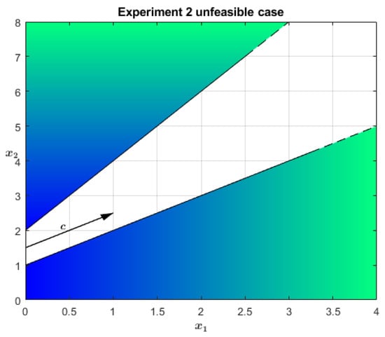
Figure 4.
Example of an empty primal polyhedron.
All in all, applying the embedding in (14), the existence of optimal primal-dual solutions is guaranteed and an implementation of the NA-IPM, which does not repeatedly check for infeasibility can be used, helping the performance a lot.
5.3. Experiment 3: Two-Objective QP
The problem faced in this subsection is nonlinear in the first objective and linear in the second one. Its formal construction is reported in Appendix A, while its standard description is in Equation (26) and its non-Archimedean one is in Equation (27):
The primal feasible region is a right square pyramid of height one, see Figure 5. Its basis lies on the plane and has its center at and vertices in , , , and . Moving to the cost function, the first objective penalizes points far from the line , , i.e., the axis of the cylinder in Figure 6. The optimal region, highlighted in green in both the figures, is the height of the furthest-from-origin face of the pyramid, identified by the intersection of the latter with the cylinder of radius and as the axis. Finally, the second objective selects from the whole apothem the point as close as possible to the plane, namely .
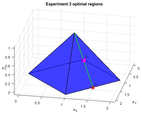
Figure 5.
The segment in green is the optimal region for the first objective and is its middle point. The starred one, , is the global optimum instead.
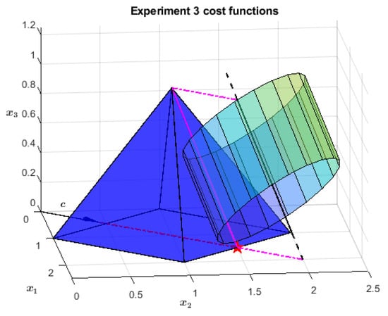
Figure 6.
Cost functions: the primary is the distance from the oblique line, each infinite cylinder is a level surface; the secondary maximizes the sum of and .
Before reaching the global optimum, the NA-IPM passes close to the midpoint of the first objective optimal region. In the current problem, it is , which is approached since iteration 3, as can be seen in Table 3. Then, starting from iteration 6, it goes towards since the algorithm perceives the first objective as fully optimized, as one can deduce from the change in magnitude of .
Table 3.
Iterations of the NA-IPM solving the problem in (27).
5.4. Experiment 4: Three-Objective QP
The last test problem involves three distinct objective functions. Again, the step-by-step construction is reported in the appendix (Appendix B to be precise), while its standard and non-Archimedean descriptions are the ones in Equations (28) and (29), respectively:
where
The feasible region is the same pyramid as in the previous problem, Section 5.3. This time, however, there are three objectives and only the first one is linear (see Figure 7). The latter promotes as optimal the whole farthest-from-origin face of the pyramid, the green one in Figure 8. The second objective is again a penalization for the distance from a line, which in this case is , . Of the original triangle, the only optimal surface for the second objective is the segment linking and , highlighted in magenta in both the figures. The third objective selects just one point of that segment: . It consists of a potential function with the shape of an infinite paraboloid, centered on and growing linearly along .
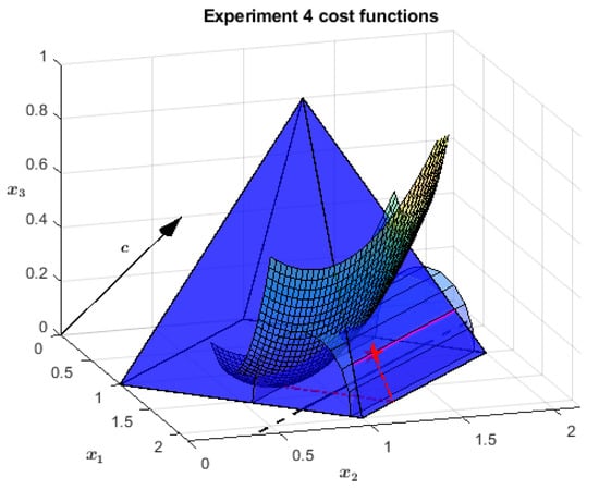
Figure 7.
Cost functions: the primary objective is the vector c; the secondary one is the distance from the black line on the axis (the cylinder is a level surface); the tertiary one is the infinite paraboloid centered on .
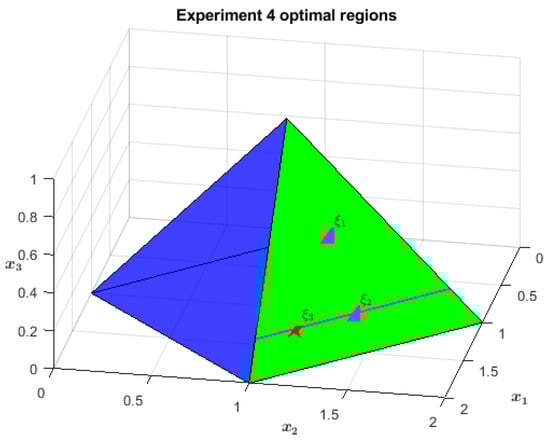
Figure 8.
The surface in green is the optimal region of the first objective ( is its midpoint); the segment in magenta is the also optimal region for the second objective ( is its midpoint); is the global optimum.
As one can imagine, the NA-IPM passes close to two more points before reaching . The first of those is the center of the green triangle, i.e., . Then, it goes towards , which would have been one of the global optima (but the unique one with maximum centrality) if the problem had had just two objectives rather than three. Indeed, it is the midpoint of the second objective optimal segment along the green triangle. Table 4 identifies this switch in the optimizing direction at iterations 5–6, when becomes infinitesimal of the first order. Eventually, the third objective takes the stage and brings the optimization away from , pointing in the direction of . This happens at iterations 10–11, when the magnitude of decreases again, making it infinitesimal of the second order. Such a value of testifies to the completion of both the first and second objective optimization, leaving space for the third.
Table 4.
Iterations of the NA-IPM solving the problem in (28).
5.5. An Informal Comparison with The Scalarization Approach
A typical standard approach to tackle (deterministic) lexicographic optimization problems is the scalarization method [18]. In terms of effectiveness, it is not able to guarantee equivalence between the original problem and the scalarized one, even if it converges to a solution significantly faster. More important, the choice of the scalarization parameters always requires a trial-and-error process to achieve good tuning: even in the case of a weighted combination of the objectives, the motto “the smaller the better” can be applied. Table 5 shows this fact quantitatively, using the benchmark in Section 5.4 as a reference problem.
Table 5.
The approximation error of the optimal lexicographic point does not monotonically decrease when reducing the scalarization weight w on problem (28).
The study replaces the non-Archimedean weight in (29) with a standard one (w), and solves the problem using the Matlab quadrprog routine. The evidence highlights how values of w that are too large or too small introduce a bias in the optimization which negatively affects the computations. Actually, the error made by the solving algorithm, i.e., the norm of the discrepancy between the theoretically optimal point and the solution found, is not acceptable even when w decreases too much. Furthermore, the scalarization approach is always problem-dependent, which means it cannot constitute a general-purpose solving paradigm.
6. Conclusions
This paper builds upon a theoretical and practical achievement that happened in the last years concerning the solution of the lexicographic multi-objective linear programming problem. Indeed, in [4], it has been demonstrated that a non-Archimedean version of the Simplex algorithm is able to solve that problem, in an elegant and powerful way. The aim of this work was to verify whether or not a non-Archimedean version of an interior point algorithm (called the NA-IPM by the authors) is able to deliver a solution to the same class of problems and go beyond it. This paper answers affirmatively, and this is interesting for situations where an interior point method is known to perform better than Simplex, such as in high-dimensional problems. With this NA-IPM at hand, it was natural to verify if it was able to solve a convex lexicographic multi-objective quadratic programming problem, and again the answer is positive.
The proposed implementation of the NA-IPM shows a polynomial complexity, and its implementation guarantees to converge in finite time. The new algorithm also enjoys a very light embedding which gets rid of the issues related to infeasibility and unboundedness. As a practical application, this paper considered and discussed lexicographic optimization problems as well as infeasible/unbounded ones, testing the NA-IPM on four linear and quadratic programming examples, and achieving the expected results. paves the way to more difficult ones, such as lexicographic multi-objective semi-definite programming problems, which are left as a future study. It should also be noted that the NA-IPM can be used to solve other families of problems involving infinitesimal/infinite numbers, as testified by Section 5.2. The study of its performances on harder examples is left for a future study as well.
Author Contributions
Conceptualization, L.F. and M.C.; Methodology, L.F.; Software, L.F.; Validation, L.F.; Formal analysis, L.F.; Investigation, L.F.; Data curation, L.F.; Writing— original draft, L.F.; Writing—review & editing, L.F. and M.C.; Visualization, L.F.; Supervision, M.C.; Project administration, M.C.; Funding acquisition, M.C. All authors have read and agreed to the published version of the manuscript.
Funding
This research was funded by the Italian Ministry of Education and Research (MIUR) in the framework of the CrossLab project (Departments of Excellence).
Acknowledgments
The authors wish to express our warmest appreciation to Vieri Benci for his generous help in teaching us Robinson’s non-standard analysis and his Alpha Theory. The authors are very thankful to the three anonymous reviewers for their accurate comments and insightful remarks.
Conflicts of Interest
The authors declare no conflict of interest.
Appendix A. Cost Function Construction in Experiment 3
This appendix shows the construction of the cost function in problem (27). The second objective discussion is omitted since it is linear and, therefore, trivial.
The idea is to make the apothem of the farthest-from-origin face of the pyramid optimal for the first objective. This segment belongs to the line , . A possible cost function is the one that penalizes the distance from a line parallel to . In addition, must satisfy the property that no point in the primal feasible region (the pyramid) is closer to it than . A feasible choice is the translation of along , say , . In this case, the line versor is .
The distance d of any point from comes from the following equation
where and is any point on , i.e., . A few lines to explain the equation follow. The translation brings the system origin to , which allows one to consistently execute the projection of the point of interest (identified by in the new reference system) along . To do this, first, one computes the norm of the projection by the inner product , then one constructs the projection by multiplying such norm by the line reference direction, that is its versor v. Since the projection of on is parallel to it by definition, the difference between and such a projection must be orthogonal to it, i.e., it is the distance of x from in the coordinate system with origin in .
In problem (27), is arbitrarily chosen as the vector ; therefore, the distance is:
To model the problem as a QP task, one can use the squared norm of the distance d as a cost function. After having done the calculations, its expression is (up to a multiplicative factor)
where k is a constant with no impact on the optimization and, therefore, it shall not be considered furthermore. Dividing (A2) by 6, one gets exactly the matrix Q and the vector q in (27) (we remind the reader that Q is divided by 2 in the cost function and, therefore, the diagonal entries must be doubled).
The optimal solution of the whole problem must lie on the pyramid face apothem due to the first objective function, i.e., for some . The second objective, namely c in (27), forces (read ) to possess another property: it must also solve the following scalar optimization problem t:
. Therefore, the optimal solution of the whole problem is , which coincides with in Section 5.3.
Appendix B. Cost Function Construction in Experiment 4
This appendix shows the construction of the cost function in problem (28). It consists of three different objectives, the first is linear while the other two are quadratic. Let us disclose them in order.
The first objective indicates as the optimal surface the whole farthest-from-origin face of the pyramidal feasible region. To select it, the cost vector c must be orthogonal to the plane the triangular face belongs to. Actually, that plane is identified by the equation , as testified by the fourth constraint in (28). Basic notions in linear algebra say that the normal direction to a plane is exactly the span of the vector filled with its coefficients, i.e., . Since the problem is a minimization one and the constraint is lesser than or equal to one, then the normal vector must be reversed, that is , exactly as in (30).
Of such an optimal face, the second objective selects just a segment parallel to the basis. To do it, the distance from a straight line is used, similarly to what is done in Appendix A. Actually, the reference line must be parallel to both the basis and the face; , is a feasible choice. Indeed, it is parallel to the plane (read the pyramid basis) since it is constant on , while it is parallel to the face because it is parallel to its basis , . Using (A1), the distance equation in this case becomes:
where and . The squared norm of the distance is now (up to a multiplicative factor)
which originates Q and q of (30).
To analytically identify the optimal region for the second objective, let one project the problem on the plane and then retrieve the whole surface, leveraging the fact that such surface is a segment parallel to . Applying the condition , the pyramid face collapses to its apothem, whose equation is , (see Appendix A). Since the optimal region must belong to , to retrieve it one has to substitute the equation of into (A3), to differentiate with respect to t and to impose the optimality condition:
Therefore, the optimal surface for the second objective is a line parallel to and passing through (by construction it already belongs to ). Basic linear algebra considerations say that this request is equivalent to constraining the sought region to the line . To identify the values of t for which belongs to the triangular face, one needs to intersect with the pyramid edges and . The intersecting points are located at and , respectively. Therefore, the optimal region for the second objective is , , henceforth indicated by .
The third objective is a potential function. By arbitrary choice, it is an infinite paraboloid centered in and growing linearly along , i.e., its equation is (scaled up for practical reasons by a factor 2)
which coincides with P and p of (30).
The optimal point of the whole problem is the point of (optimal surface identified by the second objective) which minimizes (A4). Since , it has the form , . Substituting this parametric description into (A4) and applying the first order optimality condition, one gets
Therefore, .
References
- Bazaraa, M.S.; Sherali, H.D.; Shetty, C.M. Nonlinear Programming: Theory and Algorithms; John Wiley & Sons: Hoboken, NJ, USA, 2013. [Google Scholar] [CrossRef]
- Boyd, S.; Vandenberghe, L. Convex Optimization; Cambridge University Press: Cambridge, UK, 2004. [Google Scholar] [CrossRef]
- Gondzio, J. Interior point methods 25 years later. Eur. J. Oper. Res. 2012, 218, 587–601. [Google Scholar] [CrossRef]
- Cococcioni, M.; Pappalardo, M.; Sergeyev, Y.D. Lexicographic multi-objective linear programming using grossone methodology: Theory and algorithm. Appl. Math. Comput. 2018, 318, 298–311. [Google Scholar] [CrossRef]
- Khorram, E.; Zarepisheh, M.; Ghaznavi-ghosoni, B. Sensitivity analysis on the priority of the objective functions in lexicographic multiple objective linear programs. Eur. J. Oper. Res. 2010, 207, 1162–1168. [Google Scholar] [CrossRef]
- Letsios, D.; Mistry, M.; Misener, R. Exact lexicographic scheduling and approximate rescheduling. Eur. J. Oper. Res. 2021, 290, 469–478. [Google Scholar] [CrossRef]
- Pourkarimi, L.; Zarepisheh, M. A dual-based algorithm for solving lexicographic multiple objective programs. Eur. J. Oper. Res. 2007, 176, 1348–1356. [Google Scholar] [CrossRef]
- Sherali, H.D. Equivalent weights for lexicographic multi-objective programs: Characterizations and computations. Eur. J. Oper. Res. 1982, 11, 367–379. [Google Scholar] [CrossRef]
- Hwang, C.L.; Masud, A.S.M. Multiple Objective Decision Making—Methods and Applications: A State-of-the-Art Survey; Springer Science & Business Media: Berlin/Heidelberg, Germany, 2012; Volume 164. [Google Scholar] [CrossRef]
- Arora, J. Multiobjective Optimum Design Concepts and Methods. In Introduction to Optimum Design; Elsevier: Amsterdam, The Netherlands, 2012; pp. 657–679. [Google Scholar] [CrossRef]
- Benci, V.; Cococcioni, M. The Algorithmic Numbers in Non-Archimedean Numerical Computing Environments. Discret. Contin. Dyn. Syst.-Ser. 2021, 14, 1673. [Google Scholar] [CrossRef]
- Benci, V.; Cococcioni, M.; Fiaschi, L. Non-Standard Analysis Revisited: An Easy Axiomatic Presentation Oriented Towards Numerical Applications. Int. J. Appl. Math. Comput. Sci. 2021, 32, 65–80. [Google Scholar] [CrossRef]
- Sergeyev, Y.D. Numerical infinities and infinitesimals: Methodology, applications, and repercussions on two Hilbert problems. EMS Surv. Math. Sci. 2017, 4, 219–320. [Google Scholar] [CrossRef]
- Cococcioni, M.; Fiaschi, L.; Lambertini, L. Non-Archimedean Zero Sum Games. Appl. Comput. Appl. Math. 2021, 393, 113483. [Google Scholar] [CrossRef]
- Fiaschi, L.; Cococcioni, M. Non-Archimedean Game Theory: A Numerical Approach. Appl. Math. Comput. 2020, 409, 100687. [Google Scholar] [CrossRef]
- Lai, L.; Fiaschi, L.; Cococcioni, M. Solving Mixed Pareto-Lexicographic Many-Objective Optimization Problems: The Case of Priority Chains. Swarm Evol. Comput. 2020, 55. [Google Scholar] [CrossRef]
- Lai, L.; Fiaschi, L.; Cococcioni, M.; Deb, K. Solving Mixed Pareto-Lexicographic Many-Objective Optimization Problems: The Case of Priority Levels. IEEE Trans. Evol. Comput. 2021, 25, 971–985. [Google Scholar] [CrossRef]
- Lai, L.; Fiaschi, L.; Cococcioni, M.; Kalyanmoy, D. Pure and mixed lexicographic-Paretian many-objective optimization: State of the art. Nat. Comput. 2022, 1, 1–16. [Google Scholar] [CrossRef]
- Cococcioni, M.; Cudazzo, A.; Pappalardo, M.; Sergeyev, Y.D. Solving the Lexicographic Multi-Objective Mixed-Integer Linear Programming Problem Using Branch-and-Bound and Grossone Methodology. Comm. Nonlinear Sci. Numer. Simul. 2020, 84, 105177. [Google Scholar] [CrossRef]
- Cococcioni, M.; Fiaschi, L. The Big-M Method using the Infinite Numerical M. Optim. Lett. 2021, 15, 2455–2468. [Google Scholar] [CrossRef]
- Nocedal, J.; Wright, S. Numerical Optimization; Springer Science & Business Media: Berlin/Heidelberg, Germany, 2006. [Google Scholar] [CrossRef]
- Kozlov, M.K.; Tarasov, S.P.; Khachiyan, L.G. Polynomial solvability of convex quadratic programming. Dokl. Akad. Nauk. 1979, 248, 1049–1051. [Google Scholar] [CrossRef]
- Forsgren, A.; Gill, P.E.; Wright, M.H. Interior methods for nonlinear optimization. SIAM Rev. 2002, 44, 525–597. [Google Scholar] [CrossRef]
- Mehrotra, S. On the implementation of a primal-dual interior point method. SIAM J. Optim. 1992, 2, 575–601. [Google Scholar] [CrossRef]
- Gondzio, J.; Grothey, A. Direct solution of linear systems of size 109 arising in optimization with interior point methods. In International Conference on Parallel Processing and Applied Mathematics; Springer: Berlin/Heidelberg, Germany, 2005; pp. 513–525. [Google Scholar] [CrossRef]
- Colombo, M.; Gondzio, J. Further development of multiple centrality correctors for interior point methods. Comput. Optim. Appl. 2008, 41, 277–305. [Google Scholar] [CrossRef]
- Wright, S.J. Primal-Dual Interior-Point Methods; SIAM: Philadelphia, PA, USA, 1997. [Google Scholar] [CrossRef]
- Andersen, E.D.; Andersen, K.D. Presolving in linear programming. Math. Program. 1995, 71, 221–245. [Google Scholar] [CrossRef]
- Bertsekas, D.P. Nonlinear programming. J. Oper. Res. Soc. 1997, 48, 334. [Google Scholar] [CrossRef]
- Stoer, J.; Bulirsch, R. Introduction to Numerical Analysis; Springer Science & Business Media: Berlin/Heidelberg, Germany, 2013; Volume 12. [Google Scholar] [CrossRef]
- Gonzaga, C.C. Path-following methods for linear programming. SIAM Rev. 1992, 34, 167–224. [Google Scholar] [CrossRef]
- Kojima, M.; Megiddo, N.; Mizuno, S. A general framework of continuation methods for complementarity problems. Math. Oper. Res. 1993, 18, 945–963. [Google Scholar] [CrossRef]
- Zhang, S. A new self-dual embedding method for convex programming. J. Glob. Optim. 2004, 29, 479–496. [Google Scholar] [CrossRef]
- Benci, V.; Di Nasso, M. How to Measure the Infinite: Mathematics with Infinite and Infinitesimal Numbers; World Scientific: Singapore, 2018. [Google Scholar] [CrossRef]
- Keisler, H.J. Foundations of Infinitesimal Calculus; Prindle, Weber & Schmidt Boston: Boston, MA, USA, 1976; Volume 20. [Google Scholar]
- Rossi, F.; Fiaschi, L.; Cococcioni, M.; Saponara, S. Design and FPGA Synthesis of BAN Processing Unit for non-Archimedean Number Crunching. In Applications in Electronics Pervading Industry, Environment and Society; Saponara, S., De Gloria, A., Eds.; Springer International Publishing: Cham, Switzerland, 2022. [Google Scholar]
- Megiddo, N. Pathways to the optimal set in linear programming. In Progress in Mathematical Programming; Springer: Berlin/Heidelberg, Germany, 1989; pp. 131–158. [Google Scholar] [CrossRef]
- Kojima, M.; Mizuno, S.; Yoshise, A. A primal-dual interior point algorithm for linear programming. In Progress in Mathematical Programming; Springer: Berlin/Heidelberg, Germany, 1989; pp. 29–47. [Google Scholar] [CrossRef]
- Monteiro, R.D.; Adler, I. Interior path following primal-dual algorithms. Part I: Linear programming. Math. Program. 1989, 44, 27–41. [Google Scholar] [CrossRef]
- Monteiro, R.D.; Adler, I. Interior path following primal-dual algorithms. Part II: Convex quadratic programming. Math. Program. 1989, 44, 43–66. [Google Scholar] [CrossRef]
- McShane, K.A.; Monma, C.L.; Shanno, D. An implementation of a primal-dual interior point method for linear programming. ORSA J. Comput. 1989, 1, 70–83. [Google Scholar] [CrossRef]
- Lustig, I.J. Feasibility issues in a primal-dual interior-point method for linear programming. Math. Program. 1990, 49, 145–162. [Google Scholar] [CrossRef]
- Lustig, I.J.; Marsten, R.E.; Shanno, D.F. Computational experience with a primal-dual interior point method for linear programming. Linear Algebra Its Appl. 1991, 152, 191–222. [Google Scholar] [CrossRef]
Publisher’s Note: MDPI stays neutral with regard to jurisdictional claims in published maps and institutional affiliations. |
© 2022 by the authors. Licensee MDPI, Basel, Switzerland. This article is an open access article distributed under the terms and conditions of the Creative Commons Attribution (CC BY) license (https://creativecommons.org/licenses/by/4.0/).