Abstract
The uncertainty due to road fluctuations and vision system dynamics represents a big challenge to adjusting the steering angle of autonomous vehicles (AVs). Furthermore, AVs require fast action to follow the target lane to overcome lateral deviation with minor errors. In this regard, this paper introduces a fast model predictive controller formulated based on the discrete-time Laguerre function (DTLF) to overcome the high computational burden of the traditional MPC. To improve the hybrid DTLF-MPC performance, a modern and effective dandelion optimizer (DO) strategy is used in this work, which resulted in obtaining the optimal DTLF-MPC parameters and achieving satisfactory results. Furthermore, the proposed hybrid DTLF-MPC is designed based on different algorithms in the literature to evaluate the performance of the DO. Several scenarios are discussed in this paper to confirm the effectiveness and efficiency of the proposed control strategy system against the vision system uncertainty and road fluctuations. The results emphasize that the proposed DTLF-MPC based on the DO can achieve the best damping performance for the lateral deviations with less overshoot; around 0.4533, and a settling time of around 0.01979 s compared with other algorithms.
Keywords:
model predictive control; computational techniques; dandelion optimizer; autonomous vehicles; vision system MSC:
65K99; 90C99
1. Introduction
Recently, modern transportation systems are focused on the utilization of autonomous vehicles (AVs) widely due to their stability in movement, reduced accidents, and the ability to manufacture them with different provisions to suit the required function [1,2]. However, AVs still face some challenges, and among these are the ability to control the steering angle and ensure that the AVs continue to move in a smooth and balanced manner through the application of different AV movement algorithms such as path planning and trajectory tracking [3]. Furthermore, the AVs require an effective control paradigm with a low computational burden to handle road fluctuations and vision system uncertainty issues as well as achieve good damping performance for lateral deviations [4].
In the last decades, many AV steering angle control systems have been applied, including classical and intelligent control approaches. The popular classical control approaches that are applied for AVs include the proportional integral derivative (PID) controller as well as the sliding mode control [5,6]. At the same time, intelligent control strategies are constructed with modern machine learning and fuzzy logic systems [7,8]. In [9], a PID controller is applied for the speed control of AVs with adaptive gains based on the neural network (NN) with a radial basis function. In [10], a later control of AVs is created based on PID control with NN utilizing a backpropagation strategy. However, the applied PID control approaches do not take into account the system constraints. In [11], a sliding mood control (SMC) is also employed with AVs in different environmental conditions. The applied SMC has a lot of challenges in practical implementation due to its chattering issue. In [12], a least square algorithm is utilized with the PID controller for AV path planning and following. Although, the PID controller cannot overcome some challenges of the steering angle control, especially during road curvature fluctuations. Another methodology of AV control is a nonlinear controller based on artificial intelligence (AI) algorithms. In [13], a fuzzy logic (FL) approach is utilized to improve the car following system, and it is employed with AVs moving on highways for getting a safe traffic stream. The FL-modified algorithm is also formulated with a path-following algorithm for underwater AVs in [14]. Another work introduces an FL control strategy for a mobile robot in order to track several paths [15]. However, the utilized FL control method is very complex as it needs high-capability microprocessing for implementation practically. In [16], path planning is developed for AVs based on an artificial neural network (ANN) approach. In addition, a modified ANN is employed in the AVs path following the system in [17]. However, collecting a suitable dataset for ANN training, validation, and testing is considered a complicated process as it represents a vital rule in NN performance. If the dataset is not accurate enough, the accuracy of the NN will be ineffective. Thus, these challenges open the chance to find and apply modern and effective control systems for AV applications. The model predictive control (MPC) strategy is assessed as a successful controller for various industrial systems [18,19,20,21,22]. However, the implementation of MPC requires proper devices with high processing and fast operation. So, it becomes urgently necessary to get a few parameters of MPC applicable to AVs to minimize the computational burden, as it has huge control as well as long prediction periods [23]. The orthonormal basis function, such as the Discrete-time Laguerre function (DTLF), can formulate the MPC in an effective way to overcome the MPC-wide control and prediction horizons challenges at different conditions. This DTLF can provide an MPC with fewer gains and minimizes the computational load [24,25,26]. Thus, the gains of the developed MPC with DTLF require proper tuning to enhance the system’s performance. Tuning the controller gains with AI techniques represents an effective methodology that is better than conventional techniques and trial-and-error methods [27]. There are a lot of AI algorithms utilized with autonomous systems [28,29,30]. In [31,32], the domain factors of the path-planning strategy of AVs are tuned based on a genetic algorithm (GA). Likewise, particle swarm optimization (PSO) is used to tune the unknown factors instead of the conventional method for AV path planning [33,34]. Tuning is performed for the FL parameters of AV based on the whale optimization algorithm (WOA) [35]. In addition, a hybrid mesh adaptive direct search algorithm with GA is developed for the optimization of the AV controller parameters in [36]. The developed AI techniques demonstrate effective methods for the controller gains tuning. It can achieve better performance than the traditional conventional techniques. However, these algorithms require more adjustable parameters and face a lot of challenges due to the trapping in local optimal solutions.
This work proposes a new methodology for the tuning of the proposed developed DTLF-MPC gains by a new intelligent algorithm named the Dandelion Optimizer (DO) [37]. This algorithm can provide good performance with few adjustable parameters as well as a fast convergence rate [38]. The proposed DTLF-MPC based on the DO is compared with the neural network (NNA) [39] and mayfly algorithm (MA) [40] as recent tuning algorithms. Various road curvature scenarios and parameter uncertainty are carried out to prove the performance of the formulated DTLF-MPC based on the intelligent DO technique. This work’s new contributions can be listed as:
- Introducing a new low computational burden MPC for the steering angle control of the AV considering vision system dynamics and uncertainty.
- The proposed MPC is formulated based on an orthonormal basis function named DTLF to overcome the long control and prediction horizon implementation.
- The gains of the proposed developed DTLF-based MPC are adjusted by a recent smart algorithm called a DO instead of traditional and conventional techniques.
- A new figure of demerit objective function is created to improve the performance of the AV and cover the minimization of the overshoot and settling time within the lateral deviations simultaneously.
- The developed DTLF-MPC based on the DO is compared with different algorithms in the literature.
- The effectiveness of the proposed technique is tested under different road fluctuations and vision system uncertainty.
The remaining parts of this paper are organized as follows: Section 2 demonstrates the AV system state space modeling based on the vision system. Section 3 describes the formulations of the proposed DTLF-MPC for AVs. Section 4 introduces artificial intelligence-based optimality. The results and discussions of the proposed design for the vehicle system controller are discussed in Section 5. Finally, the paper’s conclusions are presented in Section 6.
2. AV Modeling
The state-space form is utilized in this section to describe the AVs with vision system dynamics. As shown in Figure 1, the front and the rear wheels are gathered to describe the AV model as a bicycle system, where v stands for the AV velocity represented by the lateral velocity ‘vy’ in the y-direction and the longitudinal velocity ‘vx’ in the x-direction, while δf stands for the steering angle of the front wheel. The distance from the center of gravity (CoG) to the front and rear wheels is described by lf and lr, respectively.
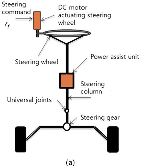
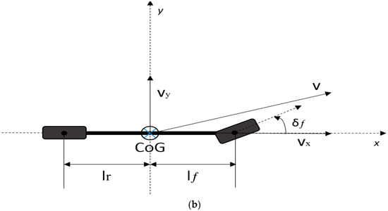
Figure 1.
The AV schematic (a) internal representation (b) a bicycle model.
The vision system provides the information related to the road as seen in Figure 2; here yL represents the lateral variation. The distance between the object and the road centerline point is described by the radius RL. KL stands for the road fluctuation, which is represented by the road radius reciprocal as ‘’. The angle within the road tangent and the orientation of AV is represented by . The look-ahead vision system distance is represented as L. The AV model in the state form is represented by the following dynamic equations [41,42]:
where,
where stands for the yaw variation of AV. While cf, cr stands for the front and rear tires cornering stiffness sequentially. The AV mass and its inertia are described by m and Iψ, respectively.
Figure 2.
The vision dynamics graphical representation (a) 3-D schematic, (b) single line description.
3. The Proposed Hybrid DTLF-MPC Formulation for AVs
The main target of the MPC is focused on finding the best control moves by adjusting the control rate ‘Δu’ within a certain control horizon ‘M’ according to the AV lateral deviation within a certain prediction horizon ‘P’. Figure 3a shows the past and current values responsible for the future output signal prediction. These output signals are used to choose the right moves by the control unit, as in Figure 3b.
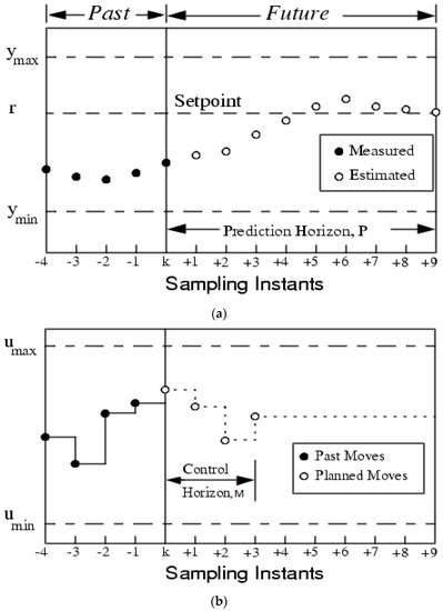
Figure 3.
The MPC prediction process (a) predicted output, (b) control moves.
The traditional MPC has the ability to predict certain points for the variations of movements ‘Δu’ for control horizon ‘M’ within this range 1 ≤ M ≤ P. However, the traditional MPC considers that ‘Δu = 0’ for the remaining points of P. The rate of control signal Δu still has small values in some cases, which mean the failure of the hypothesis of the traditional MPC [24,25,26]. This inconsistency can be tackled by giving M and P the same value, but this solution causes a huge number of calculations that require a special microcontroller with high processing for practical implementation. This paper tackles this problem by formulating the MPC based on DTLF, which is able to describe the control moves with fewer coefficients that guarantee low calculational burden as follows [23,24]:
whereas ki and k stand for the indexes of the current and future control moves, respectively. At the same time, N stands for the number of Laguerre expansion terms. The jth Laguerre function factors are described by lj and cj coefficients.
To describe the MPC control moves based on DTLF, a vector of Laguerre functions is defined as L(k)T = [l1(k), l2(k), …, lN(k)] with certain factors η = [c1, c2, …, cN]T. These factors are employed to get the proper path that can represent the control moves. The relation within Laguerre terms can be defined in the below formulations [23,24]:
as
where z stands for the pole of the DTLF network transfer function. The system stability can be confirmed by choosing ‘z’ within [0, 1]. The formulation of DTLF with the dynamic state-space model is defined in the following equation [23,24]:
where x(ki) represents the system’s initial state, Δu represents the control signal move variation. m stands for the sampling time. According to (5) and (6), the control signal is described depending on DTLF. L(i)Tη can be utilized rather than Δu(ki + i), and the dynamic system representation can be defined based on L(i)Tη as follows:
From the previous description of the dynamic system, it is clear that the new system replaces Δu, which exists in the main system, and it becomes a function in DTLF ‘η’ vector. However, there is a problem facing the controller. It is the tuning of the DTLF ‘η’ vector for providing proper control moves. This problem can be tackled by obtaining the minimum value of the following cost function [23,24]:
where Q and R are weighting vectors that balance the minimization of the error and the control effort, whereas , is the output matrix of the AV while , is a unit diagonal matrix form with dimension, N is the number of Laguerre expansion terms. q and r are unknown factors that require fine-tuning to minimize the lateral deviation. This paper utilizes the proposed intelligent DO in order to optimize the factors q and r. Furthermore, the proposed DO technique not only adjusts the weights but also the hybrid DTLF-MPC other factors, which includes the MPC sample time ‘Ts’ as well as ‘NP’, ‘N’, and ‘z’.
The following paragraph explains how to represent the vehicle model with the objective function in (9) step by step.
Step 1 Determine how to get the controller law depending on the objective function decreasing in (9)
recall (7):
as, , the following equation can be obtained by substituting (10) into (9):
The partial derivative is taken to get optimal which minimizes Equation (11), as follows:
By Solving (12):
By applying the receding horizon criteria, the following equation describes the control low
The control low can be represented as a function in the feedback signals:
where,
Step 2 Determine how to obtain the AV augment model by including an embedded integrator.
The AV dynamic equations in (1) and (2) can be converted to a discrete space model by a sample time “Ts” as shown in the following equations:
The following description can be true too:
By knowing , , and , so, (20) can be subtracted from (18) to obtain,
where .
Then, the new state variables can be defined as the new state-space form for the AV, including the embedded and known as augment model can be described as:
where, g is the output’s number, represents the unity vector with dimension, represents a zero matrix with dimension. represents the state variables number. To simplify the formulation of (23) and (24) equations can be described as follows:
where the control move is determined according to (15).
4. Artificial Intelligence-Based Optimality
Currently, artificial intelligence (AI) techniques are applied to solve many optimization challenges [43,44]. To improve the performance of the optimization techniques, AI strategies are devoted to obtaining the unknown factors depending on increasing or decreasing certain one or multiple objective functions [45,46]. The objective function can be created based on the system variables and targets [47,48]. The AI strategies are applied to obtain the best values of the gains within a certain range, taking into account the system constraints. It becomes urgently necessary to apply AI techniques because of the increasing AV system dimensions and tasks, which causes more complicated optimization issues. AI algorithms are considered intelligent solvers in many control and planning applications [49]. These techniques provide sufficient performance which exceeds the performance of the conventional method [49], but the huge number of adjusting parameters is considered the challenge which faces AI algorithm utilization in many applications. In this paper, a new AI technique named the DO is proposed to enhance the system performance with fewer adjusting parameters and it can provide sufficient results without trapping in local optima. The suggested DO technique is described in the following subsection.
In this work, a dandelion optimizer (DO) is utilized to formulate a new simplified MPC with fewer computational parameters. The dandelion optimizer is a technique utilized to simulate the dandelion seeds’ flying journey step-by-step from raising, descending, and landing steps, taking into account the weather changes. This algorithm is confirmed and tested according to the CEC2017 international standard benchmark functions [37]. The dandelion is considered one of the perennial herbs due to its simple structure, its length does not exceed 20 cm, and its flower consists of hundreds of hairs attached to small and lightweight seeds, which makes it easy to spread in the wind as it carries the seeds after its ripening season. Thanks to the crested hairs, movement parlance occurs, which makes the seeds scatter in different areas, and strong winds can carry them for tens of kilometers. So the weather condition and the wind speed are considered the main effective factors in dandelion seed spread. During the seed spread, three steps occur; the first step is the rising stage. The weather must be sunny and windy for this step to occur. The second step is the descending stage, then the landing stage. These three steps explain the modeling process of the dandelion seeds’ behavior in DO. In DO, each dandelion seed is considered a candidate solution with the population represented as [37]:
where Dim is the variable dimension and pop represents the population size. Initially, the candidate positions are created randomly within the lower bound (LB) and the upper bound (UB) for the optimization problem, and ith individual xi is represented as:
where i the index of the candidate solution and it has an integer between 1 and pop, while rand denotes a randomly distributed function that has values between [0, 1]. LB and UB are presented as LB = and . The initial elite mathematical representation can be described as follows [37]:
where and find () give equal two indexes. After the initialization, the rising process is described by considering the wind speeds in the clear days has a lognormal distribution function as . This distribution function allows more distribution for the random numbers around the Y-axis. In addition, the wind, the dandelion spread, and the speed can be utilized to update the new candidate solutions, which are formulated as follows [37]:
where, and represent a randomly selected position and dandelion seed position at the current iteration t, respectively. The randomly generated position is determined as follows [37]:
The lognormal distribution is defined by according to and , and the following equation can describe it [37]:
where y stands to the standard normal distribution within (0, 1). In the DO algorithm, an adaptive factor ‘α’ is utilized to control the length of the search process during the total number of iterations T and it is defined as follows [37]:
On rainy days, where stands to regulate the search in the local domain of the dandelion. The search domain is defined as follows [37]:
After the rising process, the descending stage starts to enhance the exploration of the DO. The moving of the dandelions trajectory is described based on Brownian motion, the position is updated after the rising stage by utilizing the information of the average as follows [37]:
where βt is a random factor determined based on the standard normal distribution and it describes the Brownian motion. While stands for the population average position in ith iteration. After descending, the landing of the dandelion seed starts as follows [37]:
where, is the dandelion seed’s optimal position during the ith iteration. is the levy flight function which is calculated by the next equation [37]:
where B is defined randomly within [0, 2]. S is a constant equal to 0.01. and t are random numbers within [0, 1] and is calculated as follows [37]:
Finally, the DO carries out the optimization process based on the above three stages in each iteration and arranges the solutions in descending order according to the fitness value from top to bottom. The agent that has the minimum fitness value represents the elite agent for the next generation of the population. Then, agents’ solutions are arranged to initialize the population for the next iteration. The optimization process is carried out until achieving the stopping condition and then brings out the best solution. The optimization process of the DO is summarized by the flowchart in Figure 4.
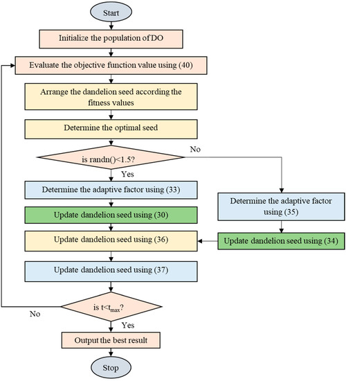
Figure 4.
The flowchart of the proposed DO.
5. Results and Discussion
This section demonstrates the DO utilization with the proposed developed DTLF–MPC technique to adjust the gains and improve the AV performance. The main requirement to improve AV performance and diminish the lateral deviation is achieved by adjusting the steering angle of the AV in order to decrease the steady state error ‘ESS’ decreasing, settling time ‘ts’, and lateral deviation maximum overshoot ‘MO’. This work provides a new figure of demerit (FoD) cost function that tackles the minimization of ‘ESS’, ‘ts’, and ‘MO’ of the lateral deviation simultaneously (Section 5 of the revised manuscript.) When the value of the FOD decreases, this means that the minimization of ‘ESS’, ‘ts’, and ‘MO’ of the lateral deviation decreases simultaneously. The formulation of the FoD cost function is described as follows [50,51]:
where represents an adjusting factor used for balancing the minimization of FoD two parts as “” concentrate on the minimization of ‘Ess’ and ‘Mo’. While this section “” focuses on decreasing ‘ts’. This work considers that equal to 0.7. This value satisfies the balance and decreasing of the cost function two parts because at the values of the weighting on the two parts are equal .
The proposed DO is utilized for the tuning of the factors of the developed DTLF-MPC to minimize the cost function in (40) as seen in Figure 5. Furthermore, the results of the DO are compared with NNA [39] and MA [40] to evaluate the system performance. Figure 6 clarifies the optimization efforts of the utilized DO versus the NNA and MA for the factors tuning the developed DTLF-MPC. In Figure 7, the values of the cost function for all algorithms are described in the chart shapes for a clearer comparison between them. Table 1 includes the developed DTLF-MPC gains, and the cost function value depends on the utilized DO, NNA, and MA. Figure 6 and Figure 7 and Table 1 clarify that the proposed DO can achieve the minimum value for the cost function with a fast convergence rate compared to NNA [39] and MA [40].
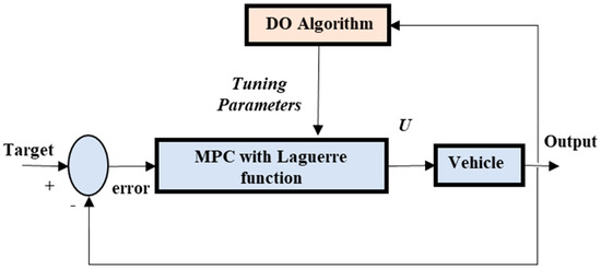
Figure 5.
The online tuning representation of the developed DTLF-MPC based on DO.
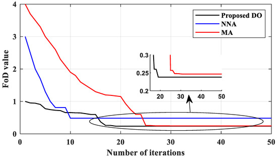
Figure 6.
The convergence effort of the applied algorithms to tune the developed DTLF-MPC gains.
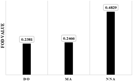
Figure 7.
The cost function value based on each technique.

Table 1.
The tuned factors of the developed DTLF-MPC depending on the applied algorithms with the corresponding cost function FoD value.
The pseudo-code in Algorithm 1 demonstrates the steps of the DO for tuning the developed DTLF-MPC gains. This developed method is tested with different road curvatures, and takes into account the big and small road curvature changes. Moreover, the proposed intelligent method is also tested with the uncertainties of the utilized system parameters. The presented outputs can prove the high performance of the utilized controller methodology.
| Algorithm 1. The pseudo-code of the DO for tuning the developed DTLF-MPC gains |
| 1: Initiate DO 2: Test the AV with the developed DTLF-MPC 3: Determine the cost function in (40) 4: while (t < T) 5: Perform the DO steps 6: Test the AV with the developed DTLF-MPC 7: Determine the cost function in (40) 8: Arrange the solutions based on the values of FoD 9: Choose the best value of FoD 10: Update the solution for the next step 11: end while 12: Stop |
From Table 1 and Figure 6 and Figure 7, the cost function values by the NNA and MA with DTLF-MPC are bigger than the cost function value by the suggested DTLF-MPC based on DO. Furthermore, the DO has a fast convergence rate compared to NAA and MA algorithms. There are many testing scenarios executed based on realistic AV data, as recorded in Table 2 [41], to prove the efficiency of the developed hybrid DTLF-MPC with DO.
Table 2.
The realistic data of the AV.
5.1. Step Disturbance Test Case
In this test case, the road curvature variation is carried out with step disturbance equal to 0.3 m−1. Figure 8 presents the system lateral variation caused by this disturbance. Figure 9 shows the ‘Mo’ and ‘ts’ values of the lateral output, which represent the output performance indexes depending on each algorithm. In Table 3, the damping characteristics of the lateral output, which is represented by ‘Mo’ and ‘ts’ are presented. The suggested hybrid DTLF-MPC developed by the DO has the ability to decrease the lateral deviation maximum overshoot with less value compared with the DTLF-MPC based on NNA and MA sufficiently. Furthermore, the lateral variation settling time decays by utilizing the developed DTLF-MPC based on the DO by 0.01979 s, less than 0.037 s and 0.09392 s by the DTLF-MPC based on MA and NNA, respectively. In addition, Figure 8 shows that the developed DO-based DTLF-MPC is able to provide high damping performance that is better than the DTLF-MPC based on NNA and MA.
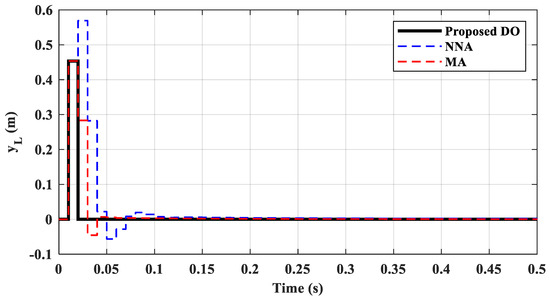
Figure 8.
The output response of the AV lateral deviation against 0.3 m−1 step disturbance in the road curvature.
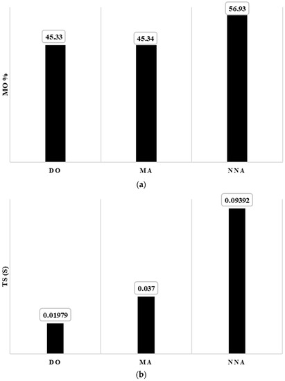
Figure 9.
The performance damping indexes due to each technique (a) the response overshoot “Mo”, (b) the response settling time “ts”.
Table 3.
The performance damping indexes including ‘Mo’ and ‘ts’ due to each technique.
5.2. Road Curvature Fluctuations Test Case
The second test case is performed to ensure that the performance of the formulated system, depending on the developed DO and hybrid DTLF-MPC, is efficient against the road curvature fluctuations challenge, especially in various disturbance cases as seen in Figure 10. The AV lateral variation response by the developed DTLF-MPC based on DO, NNA, and MA is presented in Figure 11. This figure clarifies that the response of the AV with the utilization of developed DTLF-MPC based on DO, which has the ability to damp the lateral deviation against the road curvature fluctuation with less ‘Mo’, ‘ts’, and negligible steady state error compared with other techniques.
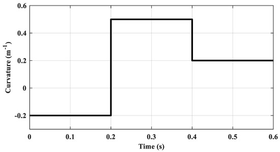
Figure 10.
Variable road curvature.
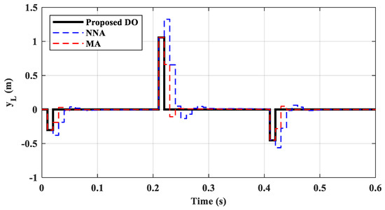
Figure 11.
The output response of the AV lateral deviation against road curvature fluctuations.
5.3. Parameter Uncertainty Test
The system parameter uncertainty caused by the measuring devices’ errors is considered a big obstacle to satisfying sufficient performance. In this test case, a ±5 m/s uncertainty in the AV velocity as well as ±5 m change in look-ahead vision distance of the vision system are created to confirm the robustness of the developed DTLF-MPC based on the DO in case of parameter uncertainty. As shown in Figure 12 and Figure 13, the output response of AV lateral deviation by developed DTLF-MPC based on the DO has the best damping performance against the parameter uncertainty compared with the DTLF-MPC based on NNA and MA. Notice that the AV has a steady-state error in the case of the DTLF-MPC based on NNA, as seen in Figure 12.
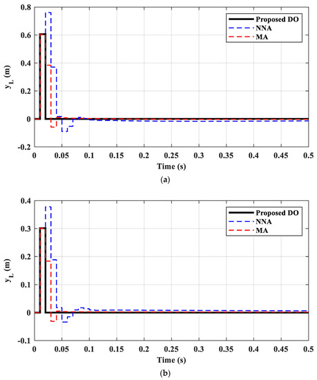
Figure 12.
The output response of the AV lateral deviation against the velocity variations (a) +5 m/s increasing, (b) −5 m/s decreasing.
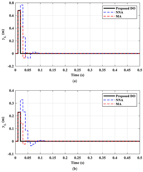
Figure 13.
The output response of the AV lateral deviation against the look-ahead distance variations of the vision system (a) +5 m increasing, (b) −5 m decreasing.
6. Conclusions
This work introduces a developed MPC with DTLF for the controlling the AV to reduce the calculational burden of the traditional MPC as well as tackle the issues of long prediction and control horizons. Besides, a new intelligent algorithm is performed for tuning the factors of the developed MPC with DTLF depending on a recent tuning algorithm named a DO instead of the conventional methods. The performance developed MPC with DTLF based on the DO is evaluated and compared with other techniques, including NNA and MA algorithms. Various test cases, including road curvature fluctuations, velocity variation, and vision system uncertainty are created to confirm the effectiveness of the developed MPC with DTLF. The output results prove the success of the developed hybrid DTLF-MPC with the DO to reduce the AV lateral deviations versus the road curvature fluctuations and the vision system uncertainty with less overshoot, around 0.4533 and settling time of around 0.01979 s compared with other algorithms. Additionally, the presented methodology provides a promising way for reducing the calculational burden of traditional MPC control, which is applicable to many industrial applications in the near future.
Author Contributions
Conceptualization, S.B. and S.-F.S.; Data curation, S.B.; Formal analysis, S.-F.S. and M.E.; Funding acquisition, M.E.; Investigation, S.-F.S. and M.E.; Methodology, S.B., S.-F.S. and M.E.; Software, S.B.; Supervision, S.-F.S.; Visualization, S.B.; Writing—original draft, S.B.; Writing—review & editing, S.-F.S. and M.E. All authors have read and agreed to the published version of the manuscript.
Funding
This work is supported by the Ministry of Science and Technology (MOST) of Taiwan, (grant number: MOST 110-2222-E-011-013).
Data Availability Statement
Not applicable.
Conflicts of Interest
The authors declare no conflict of interest.
References
- Zhang, S.; Markos, C.; James, J.Q. Autonomous Vehicle Intelligent System: Joint Ride-Sharing and Parcel Delivery Strategy. IEEE Trans. Intell. Transp. Syst. 2022, 23, 18466–18477. [Google Scholar] [CrossRef]
- Khalid, M.; Awais, M.; Singh, N.; Khan, S.; Raza, M.; Malik, Q.B.; Imran, M. Autonomous transportation in emergency healthcare services: Framework, challenges, and future work. IEEE Internet Things Mag. 2021, 4, 28–33. [Google Scholar] [CrossRef]
- Marzbani, H.; Khayyam, H.; To, C.N.; Quoc, Đ.V.; Jazar, R.N. Autonomous vehicles: Autodriver algorithm and vehicle dynamics. IEEE Trans. Veh. Technol. 2019, 68, 3201–3211. [Google Scholar] [CrossRef]
- Nam, H.; Choi, W.; Ahn, C. Model predictive control for evasive steering of an autonomous vehicle. Int. J. Automot. Technol. 2019, 20, 1033–1042. [Google Scholar] [CrossRef]
- Hernandez-Sanchez, A.; Poznyak, A.; Chairez, I. Robust proportional–integral control of submersible autonomous robotized vehicles by backstepping-averaged sub-gradient sliding mode control. Ocean. Eng. 2022, 263, 112196. [Google Scholar] [CrossRef]
- Hernandez-Sanchez, A.; Chairez, I.; Poznyak, A.; Andrianova, O. Dynamic Motion Backstepping Control of Underwater Autonomous Vehicle Based on Averaged Sub-gradient Integral Sliding Mode Method. J. Intell. Robot. Syst. 2021, 103, 48. [Google Scholar] [CrossRef]
- Miglani, A.; Kumar, N. Deep learning models for traffic flow prediction in autonomous vehicles: A review, solutions, and challenges. Veh. Commun. 2019, 20, 100184. [Google Scholar] [CrossRef]
- Aksjonov, A.; Nedoma, P.; Vodovozov, V.; Petlenkov, E.; Herrmann, M. Detection and evaluation of driver distraction using machine learning and fuzzy logic. IEEE Trans. Intell. Transp. Syst. 2018, 20, 2048–2059. [Google Scholar] [CrossRef]
- Nie, L.; Guan, J.; Lu, C.; Zheng, H.; Yin, Z. Longitudinal speed control of autonomous vehicle based on a self-adaptive PID of radial basis function neural network. IET Intell. Transp. Syst. 2018, 12, 485–494. [Google Scholar] [CrossRef]
- Han, X.; Zhang, X.; Du, Y.; Cheng, G. Design of Autonomous Vehicle Controller Based on BP-PID. In IOP Conference Series: Earth and Environmental Science; IOP Publishing: Bristol, UK, 2019; Volume 234, p. 012097. [Google Scholar]
- Nurhadi, H.; Apriliani, E.; Herlambang, T.; Adzkiya, D. Sliding mode control design for autonomous surface vehicle motion under the influence of environmental factor. Int. J. Electr. Comput. Eng. 2020, 10, 4789. [Google Scholar] [CrossRef]
- Rout, R.; Subudhi, B. Inverse optimal self-tuning PID control design for an autonomous underwater vehicle. Int. J. Syst. Sci. 2017, 48, 367–375. [Google Scholar] [CrossRef]
- González, L.; Martí, E.; Calvo, I.; Ruiz, A.; Pérez, J. Towards risk estimation in automated vehicles using fuzzy logic. In International Conference on Computer Safety, Reliability, and Security; Springer: Cham, Switzerland, 2018; pp. 278–289. [Google Scholar]
- Xiang, X.; Yu, C.; Zhang, Q. Robust fuzzy 3D path following for autonomous underwater vehicle subject to uncertainties. Comput. Oper. Res. 2017, 84, 165–177. [Google Scholar] [CrossRef]
- Mac Thi, T.; Copot, C.; De Keyser, R.; Tran, T.D.; Vu, T. MIMO fuzzy control for autonomous mobile robot. J. Autom. Control. Eng. 2016, 4, 65–70. [Google Scholar] [CrossRef][Green Version]
- Sung, I.; Choi, B.; Nielsen, P. On the training of a neural network for online path planning with offline path planning algorithms. Int. J. Inf. Manag. 2021, 57, 102142. [Google Scholar] [CrossRef]
- Peng, Z.; Wang, J. Output-feedback path-following control of autonomous underwater vehicles based on an extended state observer and projection neural networks. IEEE Trans. Syst. Man Cybern. Syst. 2017, 48, 535–544. [Google Scholar] [CrossRef]
- Du, X.; Htet, K.K.K.; Tan, K.K. Development of a genetic-algorithm-based nonlinear model predictive control scheme on velocity and steering of autonomous vehicles. IEEE Trans. Ind. Electron. 2016, 63, 6970–6977. [Google Scholar] [CrossRef]
- Kabzan, J.; Hewing, L.; Liniger, A.; Zeilinger, M.N. Learning-based model predictive control for autonomous racing. IEEE Robot. Autom. Lett. 2019, 4, 3363–3370. [Google Scholar] [CrossRef]
- Asgari, J.; Borrelli, F.; Tseng, H.E. Discussion on: “Hybrid Parameter-varying Model Predictive Control for Autonomous Vehicle Steering”. Eur. J. Control. 2008, 14, 432–434. [Google Scholar]
- Cui, Q.; Ding, R.; Zhou, B.; Wu, X. Path-tracking of an autonomous vehicle via model predictive control and nonlinear filtering. Proc. Inst. Mech. Eng. Part D J. Automob. Eng. 2018, 232, 1237–1252. [Google Scholar] [CrossRef]
- Koga, A.; Okuda, H.; Tazaki, Y.; Suzuki, T.; Haraguchi, K.; Kang, Z. Realization of different driving characteristics for autonomous vehicle by using model predictive control. In Proceedings of the 2016 IEEE Intelligent Vehicles Symposium (IV), Gothenburg, Sweden, 19–22 June 2016; pp. 722–728. [Google Scholar]
- Zheng, Y.; Zhou, J.; Xu, Y.; Zhang, Y.; Qian, Z. A distributed model predictive control-based load frequency control scheme for multi-area interconnected power system using discrete-time Laguerre functions. ISA Trans. 2017, 68, 127–140. [Google Scholar] [CrossRef]
- Wang, L. Model Predictive Control System Design and Implementation Using MATLAB®; Springer Science Business Media: Berlin/Heidelberg, Germany, 2019. [Google Scholar]
- Dileep, K.; Krishnan, S.; Jose, A. Vehicular adaptive cruise control using Laguerre functions model predictive control. Int. J. Eng. Technol. 2018, 10, 1719–1730. [Google Scholar]
- Abdullah, M.; Rossiter, J.A.; Haber, R. Development of constrained predictive functional control using Laguerre function-based prediction. IFAC-PapersOnLine 2017, 50, 10705–10710. [Google Scholar] [CrossRef]
- Joseph, S.B.; Dada, E.G.; Abidemi, A.; Oyewola, D.O.; Khammas, B.M. Metaheuristic algorithms for PID controller parameters tuning: Review, approaches and open problems. Heliyon 2022, 8, e09399. [Google Scholar]
- Fotis, G.P.; Ekonomou, L.; Maris, T.I.; Liatsis, P. Development of an artificial neural network software tool for the assessment of the electromagnetic field radiating by electrostatic discharges. IET Sci. Meas. Technol. 2007, 1, 261–269. [Google Scholar] [CrossRef]
- Winfield, A.F.; Michael, K.; Pitt, J.; Evers, V. Machine ethics: The design and governance of ethical AI and autonomous systems [scanning the issue]. Proc. IEEE 2019, 107, 509–517. [Google Scholar] [CrossRef]
- Fotis, G.; Vita, V.; Ekonomou, L. Machine learning techniques for the prediction of the magnetic and electric field of electrostatic discharges. Electronics 2022, 11, 1858. [Google Scholar] [CrossRef]
- Sarkar, R.; Barman, D.; Chowdhury, N. Domain knowledge based genetic algorithms for mobile robot path planning having single and multiple targets. J. King Saud Univ. Comput. Inf. Sci. 2020, 34, 4269–4283. [Google Scholar] [CrossRef]
- Li, Y.; Huang, Z.; Xie, Y. Research status of mobile robot path planning based on genetic algorithm. In Journal of Physics: Conference Series; IOP Publishing: Bristol, UK, 2020; Volume 1544, p. 012021. [Google Scholar]
- Li, X.; Wu, D.; He, J.; Bashir, M.; Liping, M. An Improved Method of Particle Swarm Optimization for Path Planning of Mobile Robot. J. Control Sci. Eng. 2020, 2020, 3857894. [Google Scholar] [CrossRef]
- Zhang, L.; Zhang, Y.; Li, Y. Mobile Robot Path Planning Based on Improved Localized Particle Swarm Optimization. IEEE Sens. J. 2020, 21, 6962–6972. [Google Scholar] [CrossRef]
- Manne, S.; Lydia, E.L.; Pustokhina, I.V.; Pustokhin, D.A.; Parvathy, V.S.; Shankar, K. An intelligent energy management and traffic predictive model for autonomous vehicle systems. Soft Comput. 2021, 25, 11941–11953. [Google Scholar] [CrossRef]
- Ma, H.; Li, S.; Zhang, E.; Lv, Z.; Hu, J.; Wei, X. Cooperative Autonomous Driving Oriented MEC-Aided 5G-V2X: Prototype System Design, Field Tests and AI-Based Optimization Tools. IEEE Access 2020, 8, 54288–54302. [Google Scholar] [CrossRef]
- Zhao, S.; Zhang, T.; Ma, S.; Chen, M. Dandelion Optimizer: A nature-inspired metaheuristic algorithm for engineering applications. Eng. Appl. Artif. Intell. 2022, 114, 105075. [Google Scholar] [CrossRef]
- Natarajan, E.; Markandan, K.; Sekar, S.M.; Varadaraju, K.; Nesappan, S.; Albert Selvaraj, A.D.; Franz, G. Drilling-Induced Damages in Hybrid Carbon and Glass Fiber-Reinforced Composite Laminate and Optimized Drilling Parameters. J. Compos. Sci. 2022, 6, 310. [Google Scholar] [CrossRef]
- Sadollah, A.; Sayyaadi, H.; Yadav, A. A dynamic metaheuristic optimization model inspired by biological nervous systems: Neural network algorithm. Appl. Soft Comput. 2018, 71, 747–782. [Google Scholar] [CrossRef]
- Zervoudakis, K.; Tsafarakis, S. A mayfly optimization algorithm. Comput. Ind. Eng. 2020, 145, 106559. [Google Scholar] [CrossRef]
- Kosecka, J.; Blasi, R.; Taylor, C.J.; Malik, J. Vision-based lateral control of vehicles. In Proceedings of the Conference on Intelligent Transportation Systems, Boston, MA, USA, 12 November 1997; pp. 900–905. [Google Scholar]
- Kosecka, J.; Blasi, R.; Taylor, C.J.; Malik, J. A comparative study of vision-based lateral control strategies for autonomous highway driving. In Proceedings of the IEEE International Conference on Robotics and Automation (Cat. No. 98CH36146), Leuven, Belgium, 20 May 1998; Volume 3, pp. 1903–1908. [Google Scholar]
- Goli, A.; Tirkolaee, E.B.; Aydin, N.S. Fuzzy integrated cell formation and production scheduling considering automated guided vehicles and human factors. IEEE Trans. Fuzzy Syst. 2021, 29, 3686–3695. [Google Scholar] [CrossRef]
- Elsisi, M. Optimal design of nonlinear model predictive controller based on new modified multitracker optimization algorithm. Int. J. Intell. Syst. 2020, 35, 1857–1878. [Google Scholar] [CrossRef]
- Fakhrzad, M.B.; Goodarzian, F. A new multi-objective mathematical model for a Citrus supply chain network design: Metaheuristic algorithms. J. Optim. Ind. Eng. 2021, 14, 127–144. [Google Scholar]
- Elsisi, M.; Mahmoud, K.; Lehtonen, M.; Darwish, M.M. An improved neural network algorithm to efficiently track various trajectories of robot manipulator arms. IEEE Access 2021, 9, 11911–11920. [Google Scholar] [CrossRef]
- Mokhtarzadeh, M.; Tavakkoli-Moghaddam, R.; Triki, C.; Rahimi, Y. A hybrid of clustering and meta-heuristic algorithms to solve a p-mobile hub location–allocation problem with the depreciation cost of hub facilities. Eng. Appl. Artif. Intell. 2021, 98, 104121. [Google Scholar] [CrossRef]
- Singh, P.; Choudhary, S.K. Introduction: Optimization and Metaheuristics Algorithms. In Metaheuristic and Evolutionary Computation: Algorithms and Applications; Springer: Singapore, 2021; pp. 3–33. [Google Scholar]
- Blondin, M.J. Optimization Algorithms in Control Systems. In Controller Tuning Optimization Methods for Multi-Constraints and Nonlinear Systems; Springer: Cham, Switzerland, 2021; pp. 1–9. [Google Scholar]
- Gaing, Z.L. A particle Swarm optimization approach for optimum design of PID controller in AVR system. IEEE Trans. Energy Convers. 2004, 19, 384–391. [Google Scholar] [CrossRef]
- Hekimoğlu, B. Optimal tuning of fractional order PID controller for DC motor speed control via chaotic atom search optimization algorithm. IEEE Access 2019, 7, 38100–38114. [Google Scholar] [CrossRef]
Publisher’s Note: MDPI stays neutral with regard to jurisdictional claims in published maps and institutional affiliations. |
© 2022 by the authors. Licensee MDPI, Basel, Switzerland. This article is an open access article distributed under the terms and conditions of the Creative Commons Attribution (CC BY) license (https://creativecommons.org/licenses/by/4.0/).