Daily Peak-Electricity-Demand Forecasting Based on Residual Long Short-Term Network

Abstract

Forecasting the electricity demand of buildings is a key step in preventing a high concentration of electricity demand and optimizing the operation of national power systems. Recently, the overall performance of electricity-demand forecasting has been improved through the application of long short-term memory (LSTM) networks, which are well-suited to processing time-series data. However, previous studies have focused on improving the accuracy in forecasting only overall electricity demand, but not peak demand. Therefore, this study proposes adding residual learning to the LSTM approach to improve the forecast accuracy of both peak and total electricity demand. Using a residual block, the residual LSTM proposed in this study can map the residual function, which is the difference between the hypothesis and the observed value, and subsequently learn a pattern for the residual load. The proposed model delivered root mean square errors (RMSE) of 10.5 and 6.91 for the peak and next-day electricity demand forecasts, respectively, outperforming the benchmark models evaluated. In conclusion, the proposed model provides highly accurate forecasting information, which can help consumers achieve an even distribution of load concentration and countries achieve the stable operation of the national power system.

1. Introduction

It is important to accurately forecast the electricity demand of consumers at all times based on the building’s electricity tariff structure to reduce their demand charges. In South Korea, the electricity tariff system for buildings uses the peak load demand per hour from the previous year as the contract demand and divides the demand charges into off-peak, mid-peak, and on-peak time [1]. Furthermore, the electricity-tariff system uses a method for calculating the energy charge that imposes a weighted charge on electricity-load consumption based on the amount of time electricity is used. When the maximum power used exceeds the contract demand, a surcharge of 1.5–2.5 times the basic rate is imposed based on excessive consumption [2]. Accordingly, consumers must devise strategies to avoid increased electricity surcharges, considering the energy consumption of the building and adjusting their electricity demand to prevent the peak load from exceeding the contract demand by accurately forecasting peak-usage time and amount. Additionally, consumers must attempt to shift the concentrated demand during peak-time periods through other time-zones based on an accurate electricity-demand forecast [2].

If the concentration of energy consumption exceeds the supply capacity because of a mismatch between demand and supply at the peak, it may cause significant social problems such as blackouts. Supply reserves should be secured by adding facilities, possibly involving construction and maintenance costs for additional power plants [3,4]. According to the Korea Electric Power Corporation’s (KEPCO) 2020 electricity statistics, building power sales increased from 2006 to 2020, accounting for 24% of total power sales in 2020 [5]. Additionally, peak demand is expected to increase at an average annual rate of 1.8%, with peak demand in 2034 expected to be more than 1.25 times that of 2020 [6]. Therefore, building energy consumption accounts for a significant portion of the national energy consumption, and this proportion is gradually increasing. Developing an accurate power-forecast model can reduce and distribute the peak demand of individual buildings, which is expected to help with the national power-system planning and operation by improving the regional electricity-demand concentration patterns.

Consumers must be able to forecast electricity demand for load shifting. Accordingly, the country provides public services for forecasting the electricity consumption of individual buildings, such as the KEPCO’s Power Planner and the electricity trading service provided by the Korea Power Exchange (KPX). These services help consumers forecast electricity demand and plan the power used to predict costs and electricity consumption based on future electricity demand and past consumption patterns such as the previous day and month. Most public services forecast electricity consumption based on statistical techniques, such as multiple linear regression (MLR) and customer baseline load (CBL) [7]. These public services help reduce electricity costs and enable the efficient distribution of electricity by projecting costs and consumer usage. However, the statistical models provided by public services cannot predict fluctuations in electricity demand. Excess power consumption cannot accurately help forecast electricity demand because it fluctuates depending on uncertain external factors [6]. Advanced forecasting models must learn nonlinear electricity-demand patterns and accurately predict peak demand because the statistical model used shows a large difference between the predicted and observed values.

Several studies, e.g., [8,9,10,11,12,13,14,15,16,17,18,19,20,21,22,23,24,25,26], have been conducted to improve the accuracy of the electricity-demand forecast using multivariate time-series analysis. Various methods ranging from statistical techniques that can interpret the linear relationship between input variables and observed values to machine-learning techniques that can learn nonlinear relationships have been used. A recent study [27] suggested using deep learning to design network structures in accordance with the characteristics of the input data. In particular, recurrent neural networks (RNNs) outperformed conventional machine-learning models in forecasting electricity demand through the analysis of sequence data such as the electricity demand time series, e.g., [12,13,16,17,26]. Most previous studies attempted to improve the overall forecast performance through deep-learning models, but no study has yet aimed to improve the hourly forecast performance through a deep-learning model. Thus, a new deep learning-based model needs to be developed which can improve the performance of both overall hourly electricity-demand forecasts and peak-load forecasts.

Therefore, this study proposes using residual LSTM to improve the overall predictive demand performance by minimizing residuals generated while predicting a building’s peak demand through residual learning. The proposed model uses residual blocks in the main LSTM and is implemented as residual networks. Minimizing residuals in the main LSTM can be used to map hypotheses. The proposed model was compared with deep learning-based prediction methods, such as multilayer perceptron (MLP), LSTM, CNN LSTM, and RICNN, for hourly electricity demand and peak-demand prediction to evaluate its prediction performance. The electricity-demand data collected from a building in Seoul in 2017 and 2018 were used as the dataset for training, optimizing, and validating the proposed forecast model. The main contributions of this study are summarized as follows:

• The residual LSTM can help consumers reduce demand charges by distributing the concentration of electricity demand based on accurate forecasting performance;
• The residual LSTM can help consumers in individual buildings to distribute the concentration of electricity demand during peak hours, reduce electricity demand concentration at the regional level, and contribute to the stable operation of the national power system.

2. Literature Review

In the past few years, several studies have been conducted to predict the short-term electricity load demand for buildings. The short-term demand forecast for buildings is based on statistical models, e.g., [9,15,22,24] and machine-learning models, e.g., [8,10,18,20,21,23]. Recent studies using deep learning models, e.g., [11,12,13,14,16,17,19,25,26] have improved the predictive performance.

Table 1. Literature review.

Category	Refs.	Input Variable(s)	Time Step	Method(s)	Prediction Objective
Statistical-based Modeling	[22]	Historical lighting load, Weather information, Occupant information	30 min	MLR	Peak demand
	[24]	Historical Load, Weather information, Time information	15 min	Polynomial regression, Similar day approach, MLR	Load demand
Machine learning-based modeling	[10]	Historical lighting load, Weather information, Occupant information	Hourly	ANN, SVR	Lighting load demand, Peak lighting demand
	[18]	Historical Load, Weather information	Hourly	ANN	Load demand, Peak demand
	[21]	Historical Load, Weather information	Hourly	Voting ensemble	Load demand, Peak demand
Deep learning-based modeling	[12]	Historical Load, Weather information	Hourly	LSTM	Load demand
	[13]	Historical Load	30 min	LSTM	Load demand
	[26]	Historical Load, Weather information	Hourly	LSTM	Load demand
	[16]	Historical Load, Weather information	Hourly	CNN-LSTM	Load demand
	[17]	Historical Load, Weather information, Time information	30 min	RICNN	Load demand

lists electricity demand forecasting methods that have been proposed based on the three aforementioned model categories.

Some studies have used statistical models, such as MLR or auto-regression and moving average (ARMA), to forecast building consumption demand that can learn linear relationships between variables. Fan et al., [22] predicted the peak demand of residential buildings using a general linear model (GLM) to identify which variables have the major effect on forecasting single demand peaks, obtaining a MAPE of 4.6% when forecasting peak demand in 30-min intervals. Ke et al., [24] predicted the short-term electricity load demand of campus buildings using direct curve fitting by polynomial regression, similar day approach, and MLR. After comparison, the similar day approach had a mean absolute percentage error (MAPE) of 3.37%, better than polynomial regression and MLR for direct curve fitting. When the observed relationship between the input variable and electricity demand is linear, this statistical model performs well. However, it is difficult to assign an appropriate model parameter for electricity-demand data with nonlinear relationships [3,15,28,29].

New models have been developed because of technological advancement. Machine-learning models such as artificial neural networks (ANN), support vector regression (SVR), and ensemble models have been used to learn the nonlinear relationship of electricity-demand data. Liu and Chen [10] predicted lighting energy consumption in office buildings using ANN and SVR, with an ${\mathrm{R}}^2$ of 0.9273 for SVR, indicating a higher forecast accuracy compared to ANN. Kim et al., [18] predicted the peak electricity demand of an educational building using various statistical and machine-learning forecasting models to identify which variables have a major impact on the peak-demand forecast. After comparing the performances of the different methods, the ANN resulted in a MAPE of 4.89% when forecasting hourly demand peaks, which was a higher accuracy than those of the other statistical and machine-learning models evaluated. Fan et al., [21] predicted the electricity demand of non-residential buildings using an ensemble model to improve the predictive performance of a single machine-learning model. The MAPE for the ensemble model was 2.32% for the hourly electricity-demand forecast and 2.85% for the peak-demand forecast, indicating a higher accuracy than other statistical and machine-learning models used as base learners. Therefore, the machine-learning model can learn nonlinear data relationships to improve the predictive performance of electricity demand [30]. However, because the previous machine-learning model cannot transform the model architecture based on the characteristics of the input variables [27], it cannot effectively learn the relationship between the electricity-demand observation and the exogenous variable with a time series feature.

In a recent study, deep-learning models such as LSTM and CNN were used to learn data with sequential and spatial characteristics. Luo and Oyeldele [12] employed a LSTM to study forecasting of electricity demand of educational buildings, the results of which calculated a MAE value of 2.4 for their model, which renders it more reliable than MLP, a machine-learning approach. Jin et al., [13] used LSTM to forecast electricity demand of residential buildings. They reported that LSTM, a deep-learning approach, gave lower prediction errors than MLP and SVM for their time-series data. To compare the forecast performance of various LSTM models, Ullah et al., [26] compared the electricity-demand forecast results of residential buildings using the LSTM and BILSTM. As a result, the LSTM showed higher accuracy than the BILSTM with a MAPE of 1.4574% in hourly electricity-demand forecasts. Kim and Cho [16] predicted the electricity demand of a residential building using the CNN LSTM model with a CNN layer before the LSTM layer to extract complex and difficult-to-understand features from input variables. CNN LSTM had a MAPE of 32.83%, exhibiting higher predictive performance than MLR and LSTM. Additionally, Kim et al., [17] used the RICNN model that combined the CNN layer and the LSTM layer to learn the hidden-state vector of the future and previous times to determine the electricity demand of the building complexes. The RICNN model had a MAPE of 4.48–8.79%, higher than the MLP and LSTM trained with the same data. The overall performance of these deep-learning models in forecasting electricity demand improved due to the use of model architectures consistent with the characteristics and input variables of the electricity load demand. However, previous studies that have applied deep-learning models have not aimed to enhance the performance of peak-demand forecasts.

Recent studies on the prediction of the short-term electric load demand of buildings that have suggested using deep-learning models based on LSTM or a variant of it, have demonstrated excellent performance in time-series forecasting, e.g., [12,13,16,17,26]. Such LSTM-based models can improve the accuracy when forecasting components of weather data and electricity demand by learning the relationship between the input variables and the electricity demand data [31]. However, previous studies have not considered the residual load derived from various probabilistic factors, including the behavior of the building occupants, among the components of electricity demand. The residual load, which changes probabilistically according to the behaviors, needs, and desires of occupants, is a major cause of peak demand [32]. Therefore, a method is needed for learning and predicting the pattern in the residual load to improve the performance of both peak and total electricity demand forecasting. It is expected to improve the performance of data forecasts with unexpected values by improving the performance of peak-demand forecasts.

3. Methodology

In this study, we propose the use of an LSTM-based deep learning architecture that uses a residual block to learn and accurately predict the residual load in the total electricity demand of buildings. The model learns the overall electricity demand through an LSTM layer suitable for forecasting time series, and the residual load, which is not forecast by the LSTM, through a residual block. The residual LSTM consists of a residual block, an LSTM layer, and a dense layer. First, the proposed model learns the sequential features of electricity-demand data through an LSTM layer appropriate for time series prediction. Second, the model uses the residual block to intensively learn the residual load. Finally, the model outputs the final prediction value through the dense layer. Figure 1 shows the structure of the residual LSTM proposed in this study.

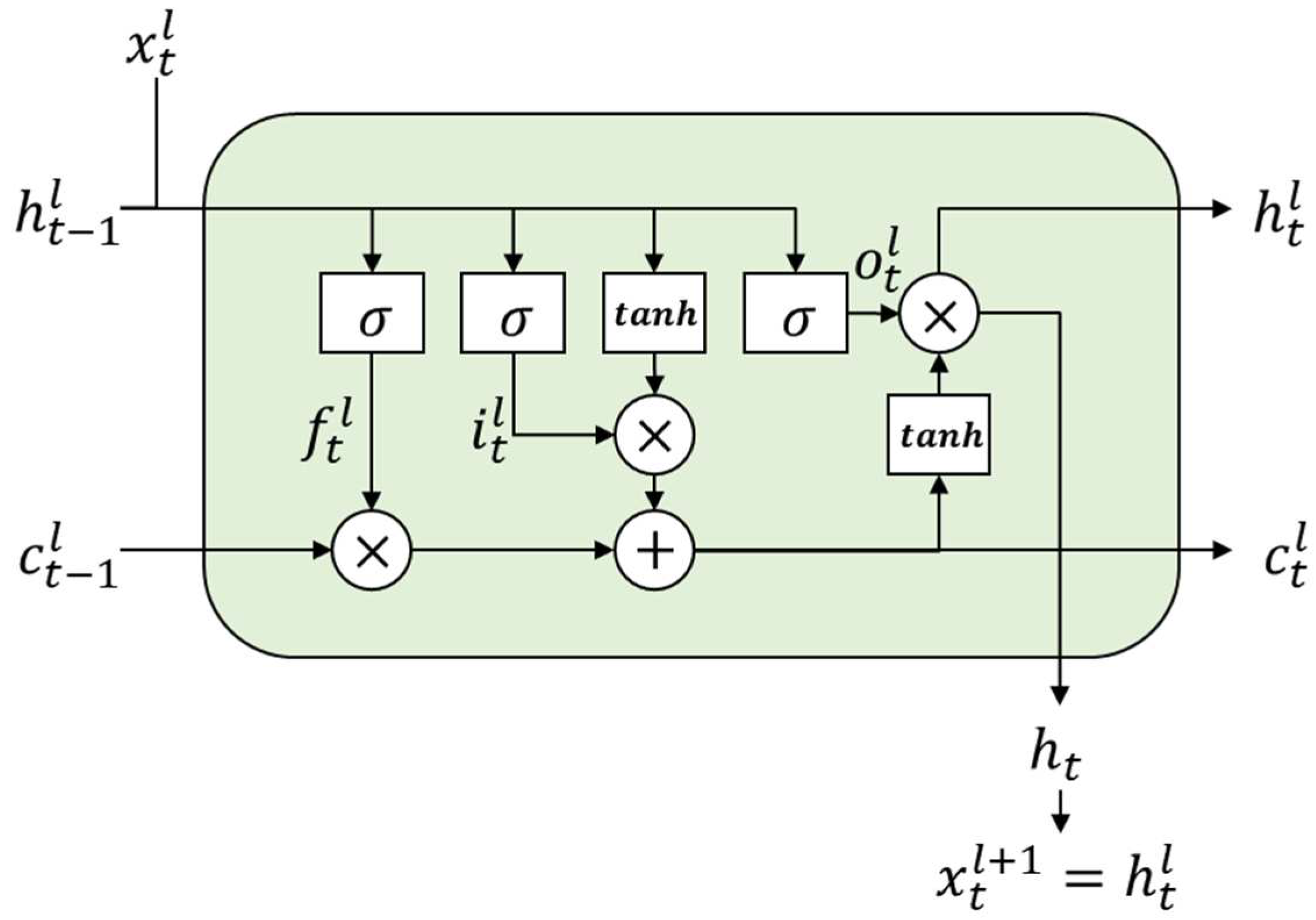
3.1. Long Short-Term Memory (LSTM)

LSTM is a variant of recurrent neural network (RNN) with modifications to the cells. A general RNN is a model suitable for learning data with recursive characteristics of storing the result calculated for each time point in the internal memory of each cell. Equation (1) is calculated in the RNN prediction process:

$$h_t=\tanh \left(W_{hh}{h}_{t-1}+W_{xh}{x}_t+b_h\right)$$

(1)

where $h_t$ denotes the output value of the RNN; $W_h$ denotes the weight; $b_h$ denotes the bias; and $x_t$ denotes the input vector. The RNN is used to calculate the output value $h_t$ of the cell at time t using the value $h_{t-1}$ calculated from the input vector $x_{t-1}$ at time t−1, which can learn the relationship between before and after data with a recursive characteristic. However, in RNN, as the network depth increases owing to the use of multiple cells, $h$ and $W_h$ are repeatedly multiplied, and the long-time gradient accumulation value decreases to zero, causing a vanishing-gradient problem [33]. LSTM uses a cell that stores a calculation result in an internal memory through input, forget, and output gates to solve this problem. Figure 2 shows the cell structure of the LSTM. Equations (2)–(8) are calculated during the LSTM prediction process.

$$f_t^l=\sigma \left(W_f^l\ast \left[h_{t-1}^l, x_t^l\right]+b_f^l\right)$$

(2)

$$i_t^l=\sigma \left(W_i^l\ast \left[h_{t-1}^l, x_t^l\right]+b_i^l\right)$$

(3)

$$o_t^l=\sigma \left(W_o^l\ast \left[h_{t-1}^l, x_t^l\right]+b_o^l\right)$$

(4)

$$c_t^l=\left(c_{t-1}^l\times f_t^l\right)+\left(\tan h(W_c^l\ast [h_{t-1}^l, x_t^l]+b_c^l\times i_t^l\right)$$

(5)

$$h_t^l=\tan h\left(c_t^l\right)\times o_t^l$$

(6)

$$\sigma \left(x\right)=\frac{1}{1+e^{-x}}$$

(7)

$$tanh\left(x\right)=1-\frac{2}{e^{2x}+1}=2\sigma \left(2x\right)-1$$

(8)

where $f_t^l$, $i_t^l$, and $o_t^l$ denote the forget, input, and output gates, respectively; $c_t^l$ denotes the cell state; $h_t^l$ denotes the cell output; $\sigma \left(x\right)$ denotes the activation function; and $tanh\left(x\right)$ denotes the hypertangent. LSTM can solve the vanishing-gradient problem through the following process. First, the forget gate decides whether to store the value of $c_{t-1}^l$ by outputting the value calculated in the previous cell as a value of zero or one. Subsequently, the input gate stores the information on $x_t$. $x_t$ stored through the input gate and the cell state $c_{t-1}^l$ at time t−1 are used to update $c_t^l$, the cell state at time t, thus facilitating using information stored through cells at a later point from the first cell to the cell at time t. Finally, the output gate outputs $h_t^l$, which is the cell’s output value at time t, using $x_t$ and $c_t^l$ updated through the input gate. Therefore, the vanishing-gradient problem can be solved by updating the cell state to prevent data with a large order difference from vanishing.

3.2. Residual Learning

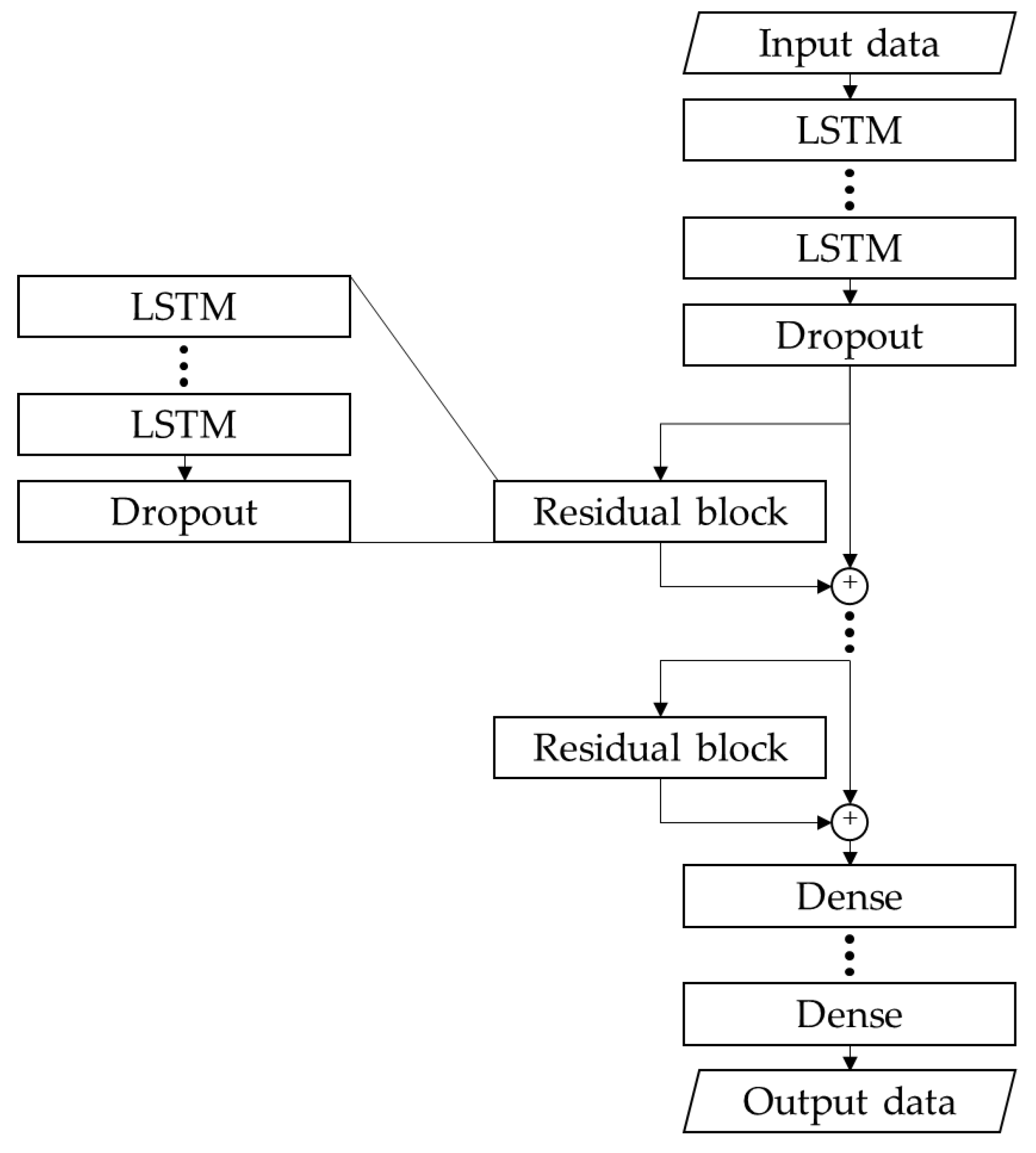
He et al., [34] presented a residual network (ResNet) as the first example of residual learning. Residual learning is performed through a residual block with a structure through which an input vector is shortcut-connected to an output layer. Figure 3a shows the structure of a normal deep learning network, while Figure 3b shows the structure of a deep learning network composed of residual blocks.

The equation for residual learning created by the residual block is expressed as follows:

$$H\left(x\right)=F\left(x\right)+x$$

(9)

where $x$ is the input vector for the first layer, $H\left(x\right)$ denotes the output function computed by the stack layer, and $F\left(x\right)$ denotes the residual function learned by a residual block. A normal deep-learning network calculates $H\left(x\right)$ to represent an input vector through a learning process. However, the deep learning network with a residual block calculates $H\left(x\right)$ as a linear combination of $F\left(x\right)$ and $x$. The result is calculated through the residual block, as shown in Equation (9).

In the backpropagation process, increasing the number of layers to improve the learning performance of a deep learning model causes a vanishing-gradient problem. Conversely, residual learning can prevent the vanishing-gradient problem by adding at least a value of one to the gradient, as the gradient value must be at least one [35,36].

3.3. Residual LSTM

Prakash et al., [37] proposed residual LSTM, using the residual block structure introduced by He et al., [34], to resolve the accuracy degradation caused by the vanishing gradient of LSTM. The proposed model consists of two LSTM layers and a shortcut connection, as shown in Figure 4, connected by a red dotted line. Additionally, an upper LSTM input vector is connected to an output layer through a skip connection.

Compared with the LSTM layer model, residual LSTM has two advantages. First, residual LSTM can learn a residual through a residual function. In the residual LSTM shown in Figure 4, the output function of the residual block is derived as Equation (10) and transformed as Equation (11):

$$H\left(x_t^l\right)=F\left(x_t^l\right)+x_t^l$$

(10)

$$F\left(x_t^l\right)=H\left(x_t^l\right)-x_t^l$$

(11)

where $H\left(x_t^l\right)$ denotes the output function of a residual block; $F\left(x_t^l\right)$ denotes the residual function; and $x_t^l$ denotes the input vector. As shown in Figure 4, $F\left(x_t^l\right)$ can be transformed into an equation that expresses the difference between $H\left(x_t^l\right)$ of the residual block and $x_t^l$, which is the same as the residual, the difference between the forecasted and observed values. Residual LSTM learns by approximating $F\left(x_t^l\right)$ to zero to $H\left(x_t^l\right)\approx x_t^l$, for finding $H\left(x_t^l\right)$ that best expresses $x_t^l$. Therefore, residual LSTM can directly learn the residual through the residual-learning process. Second, residual LSTM can solve the vanishing-gradient problem that occurs with an increasing network depth.

In the learning performance-improvement method, a deep learning model increases the network depth by adding the most representative layer. As the network depth increases, the backpropagation process encounters a vanishing-gradient problem, preventing the model parameters from being updated. The residual LSTM connects the LSTM layers of the network in parallel through a shortcut connection to allow $x_t^l$ used in the upper LSTM layer to be used in the lower LSTM layer regardless of the network depth. Therefore, residual LSTM can solve the accuracy-degradation problem of the model by solving the vanishing-gradient problem that occurs when adding the LSTM layer. A hyperparameter optimization algorithm was used to construct an optimized model architecture suitable for the experimental data. The residual LSTM adds a dropout layer that prevents the model from overfitting owing to the regularization effect [38].

4. Experimental Procedure

4.1. Data Collection and Preprocessing

This study proposed a predictive model applicable to all non-residential buildings. In South Korea, since 2017, the installation of sensors has been made mandatory in newly built or expanded public buildings of 10,000 m² or more. However, according to statistics from the Korea Energy Agency, only 128 buildings had sensors installed in 2021, with the majority having none. Therefore, this study selected a non-residential building in South Korea without sensors and examined the predictive performance of the proposed model using the building’s electricity-demand data.

To build the forecasting model proposed in this study, external data that can be collected without using a sensor other than a power meter were used as the input variables. After reviewing previous studies [9,11,14,16,17,21,23,39], we selected 17 input variables to predict the electricity demand of buildings based on the external data. Variables that affected the maximum power demand were also chosen in this study to accurately predict the maximum power demand. Different electricity rates and time zones affect peak demand because consumers try to avoid peak demand to reduce demand charges [17]. Therefore, the data for the peak-time zone of the electricity-rate system were selected as an input variable in this study. Three types of input variables were selected: (1) weather variables affecting the electricity consumption of home appliances consuming considerable power in buildings, such as air conditioners and heaters; (2) time variables affecting the repeating pattern of electricity-load consumption depending on time, date, and holidays; and (3) electricity-rate variables affecting electricity usage plans of consumers, based on electricity rates by the time of electricity use.

Table 2. Raw data input variable description.

Categories	Variable	Description	References
Weather variable	Wind speed	Wind speed (numeric)	[11,16]
	Temperature	Adjusted temperature (numeric)	[9,11,14,16,23,39]
	Humidity	Humidity (numeric)	[11,14,16,23,39]
Sequence variable	Month_x	Sine value at the month (numeric)	[15,16,21,23,39]
	Month_y	Cosine value at the month (numeric)	[15,16,21,23,39]
	Day_x	Sine value on the day (numeric)	[14,15,16,17,21,29]
	Day_y	Cosine value on the day (numeric)	[14,15,16,17,21,29]
	Hour_x	Sine value at the hour (numeric)	[11,14,15,16,23]
	Hour_y	Cosine value at the hour (numeric)	[11,14,15,16,23]
	Holiday	Weekdays/holidays status (encoded vector)	[16,21,39]
	Monday	Monday (encoded vector)	[9,11,16,17,23,39]
	Tuesday	Tuesday (encoded vector)	[9,11,16,17,23,39]
	Wednesday	Wednesday (encoded vector)	[9,11,16,17,23,39]
	Thursday	Thursday (encoded vector)	[9,11,16,17,23,39]
	Friday	Friday (encoded vector)	[9,11,16,17,23,39]
	Saturday	Saturday (encoded vector)	[9,11,16,17,23,39]
	Sunday	Sunday (encoded vector)	[9,11,16,17,23,39]
Electricity rate variable	Off-peak	Off-peak status (encoded vector)	[17]
	Mid-peak	Mid-peak status (encoded vector)	[17]
	On-peak	On-peak status (encoded vector)	[17]

presents the input variables used for the electricity-demand forecast in this study.

This study used building electricity-demand data retrieved from the power data-sharing center of KEPCO [40] to train a predictive model after de-identification. The weather variables were obtained from the Korea Meteorological Administration (KMA) weather-data open portal [41], and the electricity-rate variables were based on the KEPCO’s electricity-rate system [1]. All the data were collected hourly from 1 January 2017 to 31 December 2018. Finally, the collected data were confirmed to include more than 2000 observations, with no missing values. The collected data were normalized to an interval (0, 1) to prevent the forecast model from overlearning a specific input variable [42]. The normalization equation is as follows:

$$x^{\prime }=\frac{x-x_{min}}{x_{max}-x_{min}}$$

(12)

where $x$ denotes the original data; $x_{min}$ denotes the minimum value of $x;$ $x_{max}$ denotes the maximum value of $x;$ and $x^{\prime }$ denotes the data after normalization.

4.2. Benchmark Models

Four deep-learning models were chosen as benchmark models to validate the superiority of the proposed model. The first benchmark model was MLP, the simplest predictive model among neural networks. MLP is widely used in data mining because it can learn complex nonlinear relationships between data. Additionally, MLP was used in some related studies that predicted electricity demand [15,20].

Second, this study used LSTM as a benchmark model because it is a deep learning model designed to process sequential data. Therefore, in several studies [16,17,43], LSTM has been used as a benchmark model to verify the model proposed for time-series prediction, such as electricity demand. CNN LSTM was chosen as a benchmark model in this study because of its more complex architecture, combining CNN, LSTM, and RICNN. CNN LSTM can learn input features through CNN layers [16]. RICNN can use the hidden-state vector through the CNN layer [17]. These were chosen as benchmark models because they outperformed the LSTM model, which has been used in several studies in the electricity demand-prediction field. For brevity, detailed descriptions of the benchmark model can be found in previous studies [11,15,16,17].

4.3. Hyperparameter Setting

In this study, the hyperparameters of the proposed and benchmark models were optimized using the electricity-demand data. This study divided the data into three datasets to optimize hyper-parameters, as shown in Figure 5. The data for the 12 months of 2017 were used as the training set, the data from July to September 2018 were used as the verification set, and the data from October to December 2018 were used as the test set. Figure 5 shows that the test set was located after the validation and training sets to prevent any value from being used in the training of the proposed model [44].

In this study, the hyperparameters of the proposed and benchmark models were optimized using the grid search. The grid search applied all hyperparameter combinations to each model. During the first step, each model was trained on the training sets and then evaluated with the validation sets for the root mean square error (RMSE). The hyperparameter with the lowest RMSE was selected.

Table 3. Hyper-parameters for the proposed and benchmark models.

Model	Hyper-Parameter	Parameter Grid	Best Parameters
MLP	Epochs	[100, 200, … 5000]	500
	Batch size	[16, 32, … 512]	256
	Filter size	[16, 32, … 512]	512
	Stacks of dense layers	[1, 2, 3, 4]	4
LSTM	Epochs	[100, 200, … 5000]	100
	Batch size	[16, 32, … 512]	64
	Filter size	[16, 32, … 512]	256
	Stacks of dense layers	[1, 2, 3, 4]	1
	Stacks of LSTM layers	[1, 2, 3, 4]	2
CNN LSTM	Epochs	[100, 200, … 5000]	100
	Batch size	[16, 32, … 512]	128
	Filter size	[16, 32, … 512]	128
	Stacks of dense layers	[1, 2, 3, 4]	4
	Stacks of LSTM layers	[1, 2, 3, 4]	2
	Stacks of CNN layers	[1, 2, 3, 4]	2
	Filter size of CNN	[16, 32, … 512]	16
	Kernel size of CNN	[1, 2, 3, 4, 5, 6, 7]	1
RICNN	Epochs	[100, 200, … 5000]	200
	Batch size	[16, 32, … 512]	512
	Filter size	[16, 32, … 512]	128
	Stacks of dense layers	[1, 2, 3, 4]	4
	Stacks of LSTM layers	[1, 2, 3, 4]	2
	Stacks of CNN layers	[1, 2, 3, 4]	2
	Filter size of CNN	[16, 32, … 512]	16
RLSTM	Epochs	[100, 200, … 5000]	1000
	Batch size	[16, 32, … 512]	128
	Filter size	[16, 32, … 512]	128
	Stacks of dense layers	[1, 2, 3, 4]	2
	Stacks of LSTM layers	[1, 2, 3, 4]	2
	Stacks of residual blocks	[1, 2, 3, 4]	2
	Stacks of LSTM layers in the block	[1, 2, 3]	1
	Dropout rate	[0.1, 0.2, … 0.9]	0.8

summarizes the hyperparameter space (HP-space) of the proposed and benchmark models.

Additionally, this study made the following two adjustments to the proposed and benchmark models. Following previous studies, this study adopted the Adam optimizer [45] and mean square error (MSE) as model parameter optimization tools and the loss function as common settings [44].

4.4. Performance Measure

This study used three parameters to assess the performance of each prediction model: mean absolute error (MAE), expressed using Equation (13); MAPE, expressed using Equation (14); and RMSE, expressed using Equation (15):

$$MAE=\frac{1}{n}{\displaystyle \sum }_t^n\left|y_t-\widehat{y_t}\right|$$

(13)

$$MAPE=\frac{1}{n}{\displaystyle \sum }_t^n\frac{\left|y_t-\widehat{y_t}\right|}{y_t}\times 100$$

(14)

$$RMSE=\sqrt{\frac{1}{n}{\displaystyle \sum }_t^n{\left(y_t-\widehat{y_t}\right)}^2}$$

(15)

where$y_i$ and $\widehat{y_i}$ denote the actual and forecasted electricity consumption, respectively, at time t; and n denotes the number of observations.

5. Results and Discussion

In this study, we verify whether residual learning through residual LSTM can experimentally improve the forecast performance of the peak and overall electricity demands of buildings. The experimental results confirmed the forecast errors for peak and total electricity demands, and residual LSTM and benchmark models were compared. Accordingly, the results of the experiment are presented in this section. The results section is divided into two parts: the first section confirms the model’s peak-demand forecast results; the second confirms the total electricity demand and hourly forecast results.

5.1. Peak-Demand Forecast Results

Experiments were conducted to derive forecast performance for peak demand by aggregating peak demand among electricity demand generated during one day in the test set.

Table 4. Performance of the prediction models for the next-day peak-electricity demand.

Measure	MLP	LSTM	CNN LSTM	RICNN	RLSTM
MAE	8.71	7.16	8.32	8.28	6.86
MAPE	17.21	12.73	14.32	14.58	11.7
RMSE	11.85	10.75	11.13	12.17	10.5

The text in bold denotes the best performance for each performance measure.

presents the forecast errors for peak demand of residual LSTM and benchmark models, such as MLP, LSTM, CNN LSTM, and RICNN. These models were compared considering three error metrics: MAE, MAPE, and RMSE. Table 3 shows that residual LSTM had the best forecast performance, with the lowest error across all error metrics, demonstrating that residual learning improves peak-demand forecast performance. Meanwhile, all error metrics showed that CNN LSTM had a higher prediction error than LSTM, indicating that using a CNN method to learn relational features between input variables does not improve peak-demand forecast performance.

The accuracy of the forecast model is critical in peak-demand forecasting to ensure that the forecasted value is not underestimated. Consumers are likely to plan additional electricity usage during peak times if the predictive model underestimates peak demand. Additional electricity consumption during peak hours may result in a surcharge if consumption exceeds contract demand [20], possibly resulting in an inflated base rate because consumers choose higher contract demand than necessary during the electricity rate contracting process. Accordingly, the errors of the underestimated cases were derived in this study to confirm the performance of the underestimate in the test data at the peak time.

Table 5. Next-day forecast results when underestimated at peak times.

Measure	MLP	LSTM	CNN LSTM	RICNN	RLSTM
MAE	8.06	8.38	8.79	8.60	6.76
MAPE	14.30	12.77	13.11	13.58	9.81
RMSE	10.54	10.79	10.70	11.41	9.48

The text in bold denotes the best performance for each performance measure.

shows the forecast model error for underestimated cases at peak time, with the residual LSTM having the best predictive performance. Comparing the peak-demand-forecast results shows that residual LSTM reduced the error in all error metrics, whereas LSTM, CNN LSTM, and RICNN increased errors in some error metrics. These results indicate that the residual LSTM can predict the peak demand more accurately, particularly when peak demand is underestimated. Therefore, consumers can successfully reduce demand charges because residual LSTM prevents excessive consumption.

5.2. Overall and Hourly Forecast Results

The experiments were conducted to verify the overall results of residual LSTM. Accordingly, the forecast performances of residual LSTM and four benchmark models were compared. The overall results of peak-demand forecast performance were compared using the same three error metrics used for the peak-demand forecast.

Table 6. The performance of the prediction models for the next-day electricity demand.

Measure	MLP	LSTM	CNN LSTM	RICNN	RLSTM
MAE	5.17	4.48	3.98	4.48	3.99
MAPE	15.71	13.41	11.76	13.85	12.57
RMSE	8.46	7.7	6.95	7.73	6.91

The text in bold denotes the best performance for each performance measure.

shows the experimental results for the overall electricity-demand prediction model. In terms of MAE and RMSE, residual LSTM outperformed the benchmark models, and in terms of MAPE, residual LSTM outperformed CNN LSTM. Based on the overall performance results, residual LSTM was considered a reliable method for forecasting electricity demand with low errors.

Although an accurate overall electricity-demand forecast is important for consumers in individual buildings to establish electricity plans, an accurate forecast of peak demand helps in the distribution of the peak times. Distributing the peak in each building can help prevent the problem of energy consumption exceeding supply capacity by improving the regional electricity-demand concentration patterns. Conversely, from the perspective of the consumer and the country, the accuracy of the off-peak forecast does not significantly impact developing the electricity-usage plan. Therefore, it is necessary to examine the predictive performance for the on-peak period by dividing the period according to the energy consumption.

South Korea classifies the period for electricity use based on the total energy consumption of the country to manage the supply of energy. Electricity demand is managed by dividing the period into off-peak, mid-peak, and on-peak [1]. The period for electricity used by KEPCO is presented in

Table 7. Peak times classified by hour and month.

Demand Category	Months
	3, 4, 5, 6, 7, 8, 9	10, 11, 12, 1, 2
Off-peak	23:00–09:00	23:00–09:00
Mid-peak	09:00–10:00	09:00–10:00
	12:00–13:00	12:00–17:00
	17:00–23:00	20:00–22:00
On-peak	10:00–12:00	10:00–12:00
	13:00–17:00	17:00–20:00
		22:00–23:00

. In this study, only data from October, November, and December were used as the test set to examine the performance of the forecast model. The time zone of these three months focused on confirming the forecast performance for the on-peak periods of 10:00–12:00, 17:00–20:00, and 22:00–23:00.

Table 8. MAPE results by hour for each tested model. The text in bold denotes the best performance for each hour.

Demand Category	Time	MLP	LSTM	CNN LSTM	RICNN	RLSTM
Off-peak	00–01	5.98	5.84	4.86	10.14	7.70
Off-peak	01–02	4.50	3.90	3.61	6.20	3.79
Off-peak	02–03	2.65	4.53	3.11	5.60	3.78
Off-peak	03–04	3.42	2.66	2.02	5.26	2.11
Off-peak	04–05	2.03	4.08	3.09	5.33	4.31
Off-peak	05–06	2.73	4.16	3.36	5.95	2.46
Off-peak	06–07	2.05	3.44	2.02	7.19	1.69
Off-peak	07–08	7.79	7.99	4.15	8.46	6.73
Off-peak	08–09	32.63	27.53	22.15	24.47	20.71
Mid-peak	09–10	86.66	73.59	52.01	64.13	63.88
On-peak	10–11	215.70	181.13	133.74	166.87	119.80
On-peak	11–12	218.89	171.39	128.67	154.80	124.27
Mid-peak	12–13	155.41	117.90	84.15	110.31	102.64
Mid-peak	13–14	180.79	146.21	111.94	124.99	112.55
Mid-peak	14–15	174.24	137.29	108.60	129.43	110.62
Mid-peak	15–16	170.17	125.94	112.62	140.29	112.44
Mid-peak	16–17	132.50	120.99	120.62	140.63	97.78
On-peak	17–18	110.24	101.95	94.28	116.46	82.56
On-peak	18–19	93.40	84.51	70.68	80.30	68.48
On-peak	19–20	54.67	41.24	44.01	43.16	39.77
Mid-peak	20–21	31.19	27.05	24.44	29.76	24.21
Mid-peak	21–22	14.20	11.98	10.81	18.19	12.67
On-peak	22–23	7.76	7.60	7.80	20.68	11.62
Off-peak	23–24	9.04	8.81	7.85	17.22	9.20

The text in bold denotes the best performance for each time zone.

shows the average MAPE of the hourly forecast. Residual LSTM shows the best performance in five time steps out of six on-peak periods, indicating that residual LSTM can accurately predict power demand during on-peak periods. In mid-peak periods, residual LSTM and CNN LSTM had similar forecast performance; however, CNN LSTM had slightly better forecast performance in off-peak periods. Considering the differences in forecast performance for each period, the superiority of residual LSTM and CNN LSTM cannot be confirmed in terms of overall performance. Nevertheless, residual LSTM is a forecast model with a higher utility than other benchmark models for consumers and the country because it is capable of accurately predicting electricity demand during on-peak periods for electricity-demand management.

5.3. Statistical Tests

Using the Friedman test, we statistically compared the performance of the proposed model with those of the benchmark models. The Friedman test is a statistical method that evaluates the statistical differences between the performances of two or more forecasting algorithms [46,47]. The null (H0) and alternative (H1) hypotheses of the Friedman test are as follows:

• Null hypothesis (H0): The forecasting models have the same performance;
• Alternative hypothesis (H1): The performance of at least one model is statistically different from those of the other forecasting models.

Friedman tests with a significance level of α = 0.05 were performed for the error data of the five algorithms considered in the study.

Table 9. Friedman test results for performance of next-day electricity demand.

Compared Models			Friedman Test
n = 2208			α = 0.05
RLSTM	vs.	MLP	$H_0; e_1=e_2=e_3=e_4=e_5$
RLSTM	vs.	LSTM
RLSTM	vs.	CNN LSTM	F = 92.3
RLSTM	vs.	RICNN	P = 0.000 (Reject $H_0$)

and

Table 10. Friedman test results for performance of next-day peak-electricity demand.

Compared Models			Friedman Test
n = 92			α = 0.05
RLSTM	vs.	MLP	$H_0; e_1=e_2=e_3=e_4=e_5$
RLSTM	vs.	LSTM
RLSTM	vs.	CNN LSTM	F = 10.82
RLSTM	vs.	RICNN	P = 0.000 (Reject $H_0$)

summarize the results of these tests for the overall and peak forecast performances. The results of both tests revealed the existence of significant differences between the proposed and benchmark models.

6. Conclusions

This study proposed using residual LSTM to accurately predict the peak demand of a building to improve the forecast performance for the total electricity demand. Residual LSTM consists of an architecture in which LSTMs and residual blocks were applied for learning time-series data and residual learning, respectively. This structure allows residual LSTM to map the hypothesis more easily for the electricity demand by minimizing the residual. The proposed model was compared with existing models based on the electricity-demand data from a non-residential building considering peak-demand-forecast performance and overall forecast performance. Peak-demand forecasting shows that residual LSTM outperforms benchmark models, thus improving the overall electricity demand-forecast accuracy.

Based on the above results, the key findings and contributions of this study can be summarized as follows:

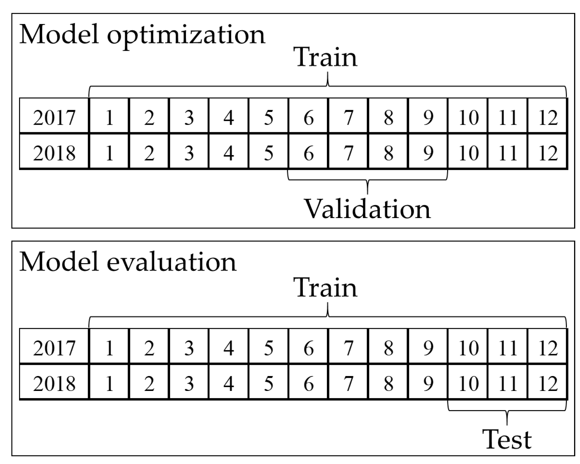
• The historical electricity demand and weather data between January 2017 and December 2018 were obtained for the area where the building used in the experiments was located;
• Three performance metrics, namely, MAPE, MAE, and RMSE, were used for assessing the performance of models when forecasting peak and next-day electricity demand;
• The peak-demand forecast by the MLP, LSTM, CNN LSTM, RICNN, and residual LSTM models were 11.85, 10.75, 11.13, 12.17, and 10.5 kW, respectively. Similarly, the RMSEs of the next-day electricity demand predicted by the models were 9.46. 7.7, 6.95, 7.73, and 6.91 kW, respectively;
• The performance evaluation of the models showed that the proposed residual LSTM was more accurate than MLP, LSTM, CNN LSTM, and RICNN in peak-demand forecasting;
• Regarding next-day electricity demand forecast, the performance of the proposed model was better for on-peak time slots with high electricity demand;
• This study demonstrates an improvement in performance when applying residual LSTM for forecasting the electricity demand of buildings;
• The proposed model can help distribute concentrated electricity demand and operation of the national power system for buildings.

For future studies, we suggest constructing predictive models for various forecast resolutions, such as a week, month, and a year later, to manage peak demand at the regional level. Second, we recommend adding a feature-selection process to the residual LSTM, which should improve the forecast performance of the model by identifying important variables while forecasting electricity demand.

References

1. Korea Electric Power Corporation. Korea Electricity Fee System. Available online: https://cyber.kepco.co.kr/ckepco/front/jsp/CY/H/C/CYHCHP00202.jsp (accessed on 4 September 2020).
2. Korea Electric Power Corporation. Korea Electricity Power Supply Terms. Available online: https://cyber.kepco.co.kr/ckepco/front/jsp/CY/D/C/CYDCHP00204.jsp (accessed on 4 September 2020).
3. Kavaklioglu, K.; Ceylan, H.; Ozturk, H.K.; Canyurt, O.E. Management. Modeling and prediction of Turkey’s electricity consumption using artificial neural networks. Energy Convers. Manag. 2009, 50, 2719–2727. [Google Scholar] [CrossRef]
4. Al-Musaylh, M.S.; Deo, R.C.; Adamowski, J.F.; Li, Y. Short-term electricity demand forecasting with MARS, SVR and ARIMA models using aggregated demand data in Queensland, Australia. Adv. Eng. Inform. 2018, 35, 1–16. [Google Scholar] [CrossRef]
5. Kim, J. Statistics of Electric Power in Korea; Korea Electric Power Corporation: Naju, Republic of Korea, 2021; Volume 90. [Google Scholar]
6. Ministry of Land, Infrastructure and Transport (MOTIE). 9th Basic Plan for Electricity Supply and Demand; South Korean Ministry of Trade, Industry and Energy: Seoul, Republic of Korea, 2020. [Google Scholar]
7. Kim, C.; Lee, C.; Park, J.; Shin, D.; Kwon, Y. Development for Evaluation and Operation Program of Demand Response Resource; Korea Electrotechnology Research Institute (KERI): Changwon, Republic of Korea, 2014. [Google Scholar]
8. Oprea, S.-V.; Bâra, A. Machine learning algorithms for short-term load forecast in residential buildings using smart meters, sensors and big data solutions. IEEE Access 2019, 7, 177874–177889. [Google Scholar] [CrossRef]
9. Vaghefi, A.; Jafari, M.A.; Bisse, E.; Lu, Y.; Brouwer, J. Modeling and forecasting of cooling and electricity load demand. Appl. Energy 2014, 136, 186–196. [Google Scholar] [CrossRef] [Green Version]
10. Liu, D.; Chen, Q. Prediction of building lighting energy consumption based on support vector regression. In Proceedings of the 2013 9th Asian Control Conference (ASCC), Istanbul, Turkey, 23–26 June 2013; pp. 1–5. [Google Scholar]
11. Wang, X.; Fang, F.; Zhang, X.; Liu, Y.; Wei, L.; Shi, Y. LSTM-based short-term load forecasting for building electricity consumption. In Proceedings of the 2019 IEEE 28th International Symposium on Industrial Electronics (ISIE), Vancouver, BC, Canada, 12–14 June 2019; pp. 1418–1423. [Google Scholar]
12. Luo, X.; Oyedele, L.O. Forecasting building energy consumption: Adaptive long-short term memory neural networks driven by genetic algorithm. Adv. Eng. Inform. 2021, 50, 101357. [Google Scholar] [CrossRef]
13. Jin, N.; Yang, F.; Mo, Y.; Zeng, Y.; Zhou, X.; Yan, K.; Ma, X. Highly accurate energy consumption forecasting model based on parallel LSTM neural networks. Adv. Eng. Inform. 2022, 51, 101442. [Google Scholar] [CrossRef]
14. Fan, C.; Wang, J.; Gang, W.; Li, S. Assessment of deep recurrent neural network-based strategies for short-term building energy predictions. Appl. Energy 2019, 236, 700–710. [Google Scholar] [CrossRef]
15. Fard, A.K.; Akbari-Zadeh, M.-R. A hybrid method based on wavelet, ANN and ARIMA model for short-term load forecasting. J. Exp. Theor. Artif. Intell. 2014, 26, 167–182. [Google Scholar] [CrossRef]
16. Kim, T.-Y.; Cho, S.-B.J.E. Predicting residential energy consumption using CNN-LSTM neural networks. Energy 2019, 182, 72–81. [Google Scholar] [CrossRef]
17. Kim, J.; Moon, J.; Hwang, E.; Kang, P. Recurrent inception convolution neural network for multi short-term load forecasting. Energy Build. 2019, 194, 328–341. [Google Scholar] [CrossRef]
18. Kim, Y.; Son, H.-g.; Kim, S. Short term electricity load forecasting for institutional buildings. Energy Rep. 2019, 5, 1270–1280. [Google Scholar] [CrossRef]
19. Cai, M.; Pipattanasomporn, M.; Rahman, S. Day-ahead building-level load forecasts using deep learning vs. traditional time-series techniques. Appl. Energy 2019, 236, 1078–1088. [Google Scholar] [CrossRef]
20. Li, K.; Hu, C.; Liu, G.; Xue, W. Building’s electricity consumption prediction using optimized artificial neural networks and principal component analysis. Energy Build. 2015, 108, 106–113. [Google Scholar] [CrossRef]
21. Fan, C.; Xiao, F.; Wang, S. Development of prediction models for next-day building energy consumption and peak power demand using data mining techniques. Appl. Energy 2014, 127, 1–10. [Google Scholar] [CrossRef]
22. Fan, H.; MacGill, I.; Sproul, A. Statistical analysis of drivers of residential peak electricity demand. Energy Build. 2017, 141, 205–217. [Google Scholar] [CrossRef]
23. Moon, J.; Kim, K.-H.; Kim, Y.; Hwang, E. A short-term electric load forecasting scheme using 2-stage predictive analytics. In Proceedings of the 2018 IEEE International Conference on Big Data and Smart Computing (BigComp), Shanghai, China, 15–18 January 2018; pp. 219–226. [Google Scholar]
24. Ke, X.; Jiang, A.; Lu, N. Load profile analysis and short-term building load forecast for a university campus. In Proceedings of the 2016 IEEE Power and Energy Society General Meeting (PESGM), Boston, MA, USA, 17–21 July 2016; pp. 1–5. [Google Scholar]
25. Rahman, A.; Srikumar, V.; Smith, A.D. Predicting electricity consumption for commercial and residential buildings using deep recurrent neural networks. Appl. Energy 2018, 212, 372–385. [Google Scholar] [CrossRef]
26. Ullah, F.U.M.; Khan, N.; Hussain, T.; Lee, M.Y.; Baik, S. Diving deep into short-term electricity load forecasting: Comparative analysis and a novel framework. Mathematics 2021, 9, 611. [Google Scholar] [CrossRef]
27. Long, W.; Lu, Z.; Cui, L. Deep learning-based feature engineering for stock price movement prediction. Knowl. Based Syst. 2019, 164, 163–173. [Google Scholar] [CrossRef]
28. Wang, Q.; Li, S.; Li, R. Forecasting energy demand in China and India: Using single-linear, hybrid-linear, and non-linear time series forecast techniques. Energy 2018, 161, 821–831. [Google Scholar] [CrossRef]
29. Reddy, S.; Akashdeep, S.; Harshvardhan, R.; Kamath, S. Stacking Deep learning and Machine learning models for short-term energy consumption forecasting. Adv. Eng. Inform. 2022, 52, 101542. [Google Scholar]
30. Bedi, J.; Toshniwal, D. Deep learning framework to forecast electricity demand. Appl. Energy 2019, 238, 1312–1326. [Google Scholar] [CrossRef]
31. Amara, F.; Agbossou, K.; Dubé, Y.; Kelouwani, S.; Cardenas, A.; Hosseini, S. A residual load modeling approach for household short-term load forecasting application. Energy Build. 2019, 187, 132–143. [Google Scholar] [CrossRef]
32. Hobby, J.D.; Tucci, G.H. Analysis of the residential, commercial and industrial electricity consumption. In Proceedings of the 2011 IEEE PES Innovative Smart Grid Technologies, Perth, WA, Australia, 13–16 November 2011; pp. 1–7. [Google Scholar]
33. Hochreiter, S.; Schmidhuber, J. Long short-term memory. Neural Comput. 1997, 9, 1735–1780. [Google Scholar] [CrossRef]
34. He, K.; Zhang, X.; Ren, S.; Sun, J. Deep residual learning for image recognition. In Proceedings of the IEEE Conference on Computer Vision and Pattern Recognition, Las Vegas, NV, USA, 27–30 June 2016; pp. 770–778. [Google Scholar]
35. Fu, S.; Zhang, Y.; Lin, L.; Zhao, M.; Zhong, S.-S. Deep residual LSTM with domain-invariance for remaining useful life prediction across domains. Reliab. Eng. Syst. Saf. 2021, 216, 108012. [Google Scholar] [CrossRef]
36. Li, M.; Li, M.; Ren, Q.; Li, H.; Song, L. DRLSTM: A dual-stage deep learning approach driven by raw monitoring data for dam displacement prediction. Adv. Eng. Inform. 2022, 51, 101510. [Google Scholar] [CrossRef]
37. Prakash, A.; Hasan, S.A.; Lee, K.; Datla, V.; Qadir, A.; Liu, J.; Farri, O. Neural paraphrase generation with stacked residual LSTM networks. ArXiv 2016, arXiv:1610.03098. [Google Scholar]
38. Alghazzawi, D.; Bamasag, O.; Albeshri, A.; Sana, I.; Ullah, H.; Asghar, M.Z. Efficient prediction of court judgments using an LSTM + CNN neural network model with an optimal feature set. Mathematics 2022, 10, 683. [Google Scholar] [CrossRef]
39. Moon, J.; Park, J.; Hwang, E.; Jun, S. Forecasting power consumption for higher educational institutions based on machine learning. J. Supercomput. 2018, 74, 3778–3800. [Google Scholar] [CrossRef]
40. Korea Electric Power Corporation. Korea Electric Power Data Open Portal System. Available online: https://www.kps.co.kr/infoopen/infoopen_03_02.do (accessed on 12 October 2020).
41. Korea Meteorological Agency. Weather Data Open Portal. Available online: https://data.kma.go.kr/data/grnd/selectAsosRltmList.do;jsessionid=w0E6ERBFNrhoVxhbDaIjpBYwiIPBZRq0koakrSIfQuCieXieb1EZZqtXC8ZJfEf9.was01_servlet_engine5?pgmNo=36 (accessed on 5 October 2020).
42. Li, K.; Su, H.; Chu, J. Forecasting building energy consumption using neural networks and hybrid neuro-fuzzy system: A comparative study. Energy Build. 2011, 43, 2893–2899. [Google Scholar] [CrossRef]
43. Mughees, N.; Mohsin, S.A.; Mughees, A.; Mughees, A. Deep sequence to sequence Bi-LSTM neural networks for day-ahead peak load forecasting. Expert Syst. Appl. 2021, 175, 114844. [Google Scholar] [CrossRef]
44. Koehn, D.; Lessmann, S.; Schaal, M. Predicting online shopping behaviour from clickstream data using deep learning. Expert Syst. Appl. 2020, 150, 113342. [Google Scholar] [CrossRef]
45. Kingma, D.P.; Ba, J. Adam: A method for stochastic optimization. ArXiv 2014, arXiv:1412.6980. [Google Scholar]
46. Verma, A.; Ranga, V. Machine learning based intrusion detection systems for IoT applications. Wirel. Pers. Commun. 2020, 111, 2287–2310. [Google Scholar] [CrossRef]
47. Jeong, J.; Kim, C. Comparison of Machine Learning Approaches for Medium-to-Long-Term Financial Distress Predictions in the Construction Industry. Buildings 2022, 12, 1759. [Google Scholar] [CrossRef]
Figure 1. Architecture of residual LSTM.
Mathematics 10 04486 g001
Figure 2. Cell structure of LSTM.
Mathematics 10 04486 g002
Figure 3. Comparison of deep learning network: (a) Normal deep-learning network; (b) Deep learning network with residual block.
Mathematics 10 04486 g003
Figure 4. Structure of residual LSTM.
Mathematics 10 04486 g004
Figure 5. Model validation and evaluation.
Mathematics 10 04486 g005