Abstract
When solving complex constrained problems, how to efficiently utilize promising infeasible solutions is an essential issue because these promising infeasible solutions can significantly improve the diversity of algorithms. However, most existing constrained multi-objective evolutionary algorithms (CMOEAs) do not fully exploit these promising infeasible solutions. In order to solve this problem, a constrained multi-objective optimization evolutionary algorithm based on the dynamic constraint boundary method is proposed (CDCBM). The proposed algorithm continuously searches for promising infeasible solutions between UPF (the unconstrained Pareto front) and CPF (the constrained Pareto front) during the evolution process by the dynamically changing auxiliary population of the constraint boundary, which continuously provides supplementary evolutionary directions to the main population and improves the convergence and diversity of the main population. Extensive experiments on three well-known test suites and three real-world constrained multi-objective optimization problems demonstrate that CDCBM is more competitive than seven state-of-the-art CMOEAs.
MSC:
68W50; 68T05
1. Introduction
Practical applications often involve constrained multi-objective optimization problems, which usually contain multiple conflicting objectives and constraints. Without loss of generality, minimizing constrained multi-objective optimization problems (CMOPs) can be formulated as follows [1]:
where F(x) is an objective function that contains m objectives and x = (, , …, ) is a d-dimension solution in the decision space . and are inequalities and equality constraints whose quantities are p and q, respectively. Usually, the constraint violation of x for the jth constraint is calculated as follows [2]:
where is a positive constraint boundary relaxation factor (usually taken as 1e-6). The overall constraint violation value of x (CV) can be summarized as:
The feasibility of a solution can be determined based on the constraint total violation CV. If the overall constraint violation (CV(x)) of one solution is zero, then it is called a feasible solution; otherwise, it is an infeasible solution. Given two feasible solutions and ∊ Ω, is said to dominate if () ≤ () for every i ∊ {1,…, m} and ()≺ () for at least one j ∊ {1, …, m}, denoted as ≺ . When a solution is not dominated by any other feasible solutions, the solution is called a feasible non-dominated solution or Pareto optimal solution. In the objective space, all Pareto optimal solutions are called the Pareto optimal solution set (PS), and the mapping of the Pareto optimal solution set in the objective space is called the Constrained Pareto Front (PF). The key to solving CMOPs is finding a set of feasible solutions with well-convergence (find Pareto optimal fronts solutions as many as possible) and well-distribution (found the solution covers all PF surfaces as many as possible) to approximate the PF [3]. For CMOPs, the objective space contains two Pareto optimal fronts, depending on whether the constraints are considered or not. In order to distinguish between them, the constrained Pareto front (CPF) and the unconstrained Pareto front (UPF) are usually used to represent the PF of the constrained multi-objective optimization problem and the unconstrained multi-objective optimization problem, respectively. Earlier researchers classified CMOPs into four categories based on the relationship between UPF and CPF [4]. These categories are (1) type-I: CPF is the same as UPF, (2) type-II: CPF is part of UPF, (3) type-III: CPF and UPF partially overlap, and (4) type-IV: CPF is wholly separated from UPF.
The challenge of constrained multi-objective evolutionary algorithms (CMOEAs) in solving CMOPs is to maintain a better balance between objective optimization and constraint satisfaction to achieve better convergence [5]. For conflicting objectives and constraints, if constraints are prioritized more than objectives, the population may quickly fall into the local feasible regions, unable to approach the true PF (especially when large infeasible regions block feasible areas). On the other hand, if objectives are prioritized more than constraints, the exploration ability of the solution is improved to a certain extent, but the convergence quality of the population may be reduced. Consequently, balancing the conflict between objectives and constraints in the evolutionary process is crucial.
Among the algorithms for solving CMOPs, the most widely used and the most typical category is the Constrained Dominance Principle (CDP) algorithm [6]. The CDP algorithm pays more attention to the feasibility of the solution (constraints have higher priority) and prefers to choose feasible solutions over infeasible solutions. Therefore, when a large infeasible area blocks the feasible area, the convergence performance of this kind of algorithm decreases. Some existing dual-population optimization algorithms cannot effectively solve CMOPs [7,8] whose optimal region is far from UPF because the auxiliary population cannot continuously maintain and utilize promising infeasible solutions during the evolution process. Furthermore, complex constraints lead to large infeasible regions between feasible regions, and small and discontinuous feasible regions make it difficult to search the population. Therefore, it is necessary to use promising infeasible solutions (CV < ) reasonably and continuously in the evolution process to help the main population pass through the infeasible region and search for a narrow potential feasible region.
Following this idea, this paper proposes dual-population based evolutionary algorithm CDCBM:
- An auxiliary population state detection strategy is proposed, which can detect the relationship between the auxiliary population and the boundary of the feasible region. According to the detected results, the auxiliary population is effectively selected in the evolution process, and more useful objective information is provided for the main population.
- For the auxiliary population, a dynamic constraint boundary method is proposed, which uses various promising infeasible solutions (CV < ) to break through the infeasible obstacles, helps the population to overcome the obstacles in the infeasible area, and makes full use of the infeasible areas approaching the feasible area. The favorable information about the solution can be used to search for potential feasible regions.
2. Materials and Methods
2.1. Related Work
This section introduces existing CMOEAs with constraint handling techniques (CHT) [9].
Early MOEAs solved CMOPs based on feasibility. For example, NSGA-II [6] is one of the most representative CDP-embedded algorithms. In the CDP method, when individuals A and B are both feasible solutions, the one with a smaller objective value enters the next generation. For a feasible solution A and an infeasible solution B, the feasible solution A is better than the infeasible solution B. For the two infeasible solutions A and B, the individual with a smaller CV value is selected. In other words, the method prefers feasible solutions to infeasible solutions. When CMOPs have discrete feasible regions or infeasible obstacles, NSGA-II [6] quickly converges to local feasible regions. To address this problem, ToR [10] uses a dual-rank fitness function that combines the CDP and Pareto strengths to evaluate the fitness of each solution by the weighted sum of the two ranks. However, the weights it constrains are always higher than the objective, which may lead to insufficient diversity. In [11], the decomposition-based MOEA (MOEA/D) and CDP were combined to form the MOEA/D-CDP method. Fan et al. [12] designed a novel angle-based CDP (ACDP) for CMOPs, which guides environment selection by measuring the angle between the parent and the corresponding child, further exploiting the information of the infeasible solutions. However, it is difficult for this method to achieve a good balance between objectives and constraints, which inevitably leads to premature convergence.
Several researchers have developed multistage CMOEAs to balance objective and constraint satisfaction. The Push-Pull Strategy (PPS) [13] is representative of a two-stage algorithm, where the goal of the push stage is to reach the UPF across infeasible regions. In the pull phase, the population is updated considering all constraints so that the population converges to the CPF. Similarly, Liu et al. [14] proposed a two-stage framework (ToP), where the first stage mainly looks for promising feasible regions, and the second stage looks for the CPF by strengthening convergence. However, there are certain difficulties in converting the first stage to the second stage. The MSCMO [15] algorithm gradually adds constraints during evolution, maintaining the diversity of the population by using the solutions found in the previous stage. Zhu et al. [16] developed an algorithm based on a detection-escape strategy, which guides the population search and escapes the stagnation state by adjusting the weight of CVs when detecting that the population search stagnates and falls into a local optimum. Tian et al. [5] adjusted the search behavior of the population according to the proportion of feasible solutions. Objective and constraint satisfaction are considered equally important in evolution when the proportion of feasible solutions for the population is less than λ. When the feasible solution is larger than λ, the constraint is given higher priority.
Some multiple population CMOEAs also involve resolving the conflict between goals and constraint satisfaction. For example, Li et al. [8] designed a dual-archive evolutionary algorithm (C-TAEA), which includes a convergence-oriented archive (CA) and a diversity-oriented archive (DA). The CA considers both objectives and constraints and mainly tends to approximate the CPF. The DA does not consider any constraints and aims to explore areas underutilized by the CA. Most of the offspring generated by the population is in the region between the UPF and CPF, which has poor convergence and diversity. Tian et al. [7] proposed a co-evolutionary framework for constrained multi-objective optimization (CCMO), where the first population is used to search for the CPF, and the second population ignores constraints to search for the UPF. The algorithm achieves better results on CMOPs with a high correlation between the CPF and UPF but poor performance on CMOPs when the UPF and CPF are far from each other. Ming et al. [17] proposed a DD-CMOEA algorithm with dual phases (i.e., exploration and exploitation) and dual population characteristics. The main and auxiliary populations are responsible for exploring feasible and infeasible solutions. Although the promising infeasible solutions obtained by the auxiliary population can help the main population to converge better, there is a lack of search for some parts of the PF, resulting in not-so-good performance. c-DPEA [18] is a co-evolutionary algorithm in which two populations use different methods to deal with infeasible solutions. Population 1 and Population 2 adopt a new adaptive penalty function and feasibility-oriented method to deal with infeasible solutions, respectively. However, the latter stages of Population 2 do not provide sufficiently diverse solutions for Population 1. Zou et al. [19] proposed a dual-population algorithm based on alternative evolution and degeneration for solving CMOPs. It can make good use of its secondary population and alternative between evolution and degeneration according to the state of the secondary population to provide good information about the secondary population to the main population. In EMCMO [20], the optimization of traditional CMOPs is transformed into two related tasks: one task targets the original CPF, and the other task ignores all constraints and only considers the objective. The responsibility of the second task is mainly to continuously provide helpful knowledge of the target to the first task, thereby facilitating the resolution of CMOPs.
Although these multiple population CMOEAs utilize infeasible solutions to maintain the diversity of the main population while exhibiting good performance on some CMOPs, there are still certain difficulties in solving complex constrained problems. The main reason is that the auxiliary population cannot continuously provide effective information during the evolution process. Aiming at this problem, we propose a method of dynamically constrained boundaries, which can continuously provide promising infeasible solutions for the main population and improve its convergence and diversity.
2.2. Methods
As shown in Table 1, all the variables used by the algorithm are presented.

Table 1.
Variables used in the algorithm.
Algorithm 1 gives the pseudo-code of CDCBM (a constrained multi-objective optimization evolutionary algorithm based on the dynamic constraint boundary method). First, two initial populations, P1 and P2, are randomly generated in the search space, and each population has N individuals. Then, in lines 5–6 of the algorithm, the binary competition selection method is used to select from select mating parent sets in P1 and P2. Then new solutions are generated by simulating binary crossover [21] and polynomial mutation [22], denoted as O1 and O2, respectively. We can see no interaction between the two populations during the initialization phase to generate offspring. Then, we need to detect whether P2 has reached UPF. Since P2 does not consider any constraint, when the sum of the current objective values of the population differs little from the previous generation, P2 enters the steady state, which can also be said to reach UPF. Therefore, we introduced a minimal parameter (1e-3 in this paper). And is the difference between the sum of all individual objective values of the current generation and that of the previous generation. If the is less than the set threshold, there is no dominant solution in P2. At this time, the value is infinite, so it can be considered that P2 reaches the UPF. When P2 reaches the UPF, the algorithm goes to lines 9–10 and sets the value to be the average of the constraint violation values in P2. Then, calculate the ratio f (the ratio of solutions (CV<=0) in P2). When f = 1, all the individuals in P2 are feasible solutions. It means that all the UPFs in P2 are at the boundary of the feasible region. Thus, we judge the relationship between the auxiliary population and the boundary of the feasible region by the results of comparing f with λ (1 in this case).
| Algorithm 1: Procedure of CDCBM |
| Input: N (population size), (sum of overall objective values of k generation in P2), Nc (proportion of nondominated solutions in P2); Output: P1(final population);
|
Algorithm 1 gives the pseudo-code of CDCBM (a constrained multi-objective optimization evolutionary algorithm based on the dynamic constraint boundary method). First, two initial populations, P1 and P2, are randomly generated in the search space, and each population has N individuals. Then, in lines 5–6 of the algorithm, the binary competition selection method is used to select from select mating parent sets in P1 and P2. Then new solutions are generated by simulating binary crossover [21] and polynomial mutation [22], denoted as O1 and O2, respectively. We can see no interaction between the two populations during the initialization phase to generate offspring. Then, we need to detect whether P2 has reached UPF. Since P2 does not consider any constraint, when the sum of the current objective values of the population differs little from the previous generation, P2 enters the steady state, which can also be said to reach UPF. Therefore, we introduced a minimal parameter (1e-3 in this paper); is the difference between the sum of all individual objective values of the current generation and that of the previous generation. If the is less than the set threshold, there is no dominant solution in P2. At this time, the value is infinite, so it can be considered that P2 reaches the UPF. When P2 reaches the UPF, the algorithm goes to lines 9–10 and sets the value to be the average of the constraint violation values in P2. Then, calculate the ratio f (the ratio of solutions (CV<=0) in P2). When f = 1, all the individuals in P2 are feasible solutions. It means that all the UPFs in P2 are at the boundary of the feasible region. Thus, we judge the relationship between the auxiliary population and the boundary of the feasible region by the results of comparing f with λ (1 in this case).
In lines 12–16 of the algorithm, after P2 converges to UPF, the value is gradually reduced by the descending speed control parameter [13], is taken as 0.05 in this paper. updates are critical to the environmental selection of P2. When decreases to a minimal threshold (1e-4 in this paper), we use a modified sigmoid function to update . a is also declining with evolutionary generations, and a ∊ [0, 1]. In this step, we update the value of back and forth between 0 and a to maintain the promising infeasible solutions in P2 and search for potentially feasible regions. The calculation of the constraint tolerance a is as follows:
where T is the current generation and (the setting in this paper is 300,000) is the maximal generation. When the value of is less than its minimum threshold (1e-4 in this paper), it means that the CV of the P2 is close to 0. At this time, by gradually reducing the constraint tolerance with the evolutionary generation, P2 retains some infeasible solutions with good objective values. With this operation, P2 searches back and forth between UPF and CPF to advance the population to the feasible region.
Inspired by [20], in the evolutionary process, selecting appropriate parental individuals and offspring individuals to enter the population for the next update can effectively save the number of evaluations. Therefore, we improve on [20] by designing an auxiliary population state detection strategy. In [20] the evolution process is simply divided into two stages, the first stage accounts for one-fifth of the entire evolution process. On the contrary, we approximate the relationship between UPF and CPF by calculating the ratio f of individuals after the auxiliary population converges to UPF. If f is equals to λ (1 in this case), the algorithm executes lines 18–21; otherwise, it enters Algorithm 2. When f is equals to λ, it indicating that the auxiliary population has entered a stable state. At this time, all solutions in the auxiliary population are feasible solutions. It is approximately determined that the UPF and the CPF coincide. After estimating the state of the auxiliary populations, the offspring O1 and O2 generated by the population are merged into the two parent generations for environmental selection. P1 uses the CDP method for environment selection, and P2 uses the method to select a new P2. In fact, at this point, = 0, which has the same effect as the CDP method. If f is not equal to λ, enter Algorithm 2. At this time, since the solutions on the CPF are feasible solutions, while most of the solutions of the auxiliary population are infeasible solutions. It is approximately judged that the UPF and the CPF are wholly or partially separated.
| Algorithm 2: Procedure of CDCBM |
| Input: N (population size), P1, P2; Output: P1;
|
In lines 1–4 of Algorithm 2, P1 and O1, and P2 and O2 are merged, respectively, to obtain a new population with 2N individuals and . Next, uses the method to select the best N individuals, and uses the CDP method to select. In this step, we want to select the more suitable parent or offspring from to participate in the interaction with P2, so method is chosen; we want to select the more suitable parent or offspring from to participate in the interaction with P1, Thus the method is chosen. Then, the success rate of the parent and offspring populations entering the next iteration is calculated according to Equations (5) and (6). The success rate of parent and child is calculated as follows:
Among them, and represent the success rates of and , respectively; and are the numbers of parents and offspring in the best N individuals. When j = 1, if < , it means that the offspring is more suitable than the parent to be selected for the next evolutionary update. In this case, O1 is kept in the temporary population TrP2. Otherwise, P1 is the better choice. The operation of j = 2 is the same as the operation of j = 1. Finally, the CDP method and the ε method are used to select the environment for P1 and P2, respectively. The interaction of populations in Algorithm 2 differs in selection from that in Algorithm 1. The reason is that when f = 1 in Algorithm 1, it means that UPF is the same as CPF, and the category is type-I [4]. When f is not equal to 1, the relationship between UPF and CPF is one of type-II: CPF is part of UPF, type-III: CPF and UPF partially overlap, and type-IV: CPF is wholly separated from UPF. Thus, in order to more efficiently select populations to enter the next generation of updates, we used a population success rate to judge.
2.3. Average Runtime and Computational Complexity
Table 2 shows the average running time of each algorithm on different test suites. We can see that the running time of CDCBM is not outstanding. The reason for this result is that all the operators are executed twice in one generation and CDCBM will consume more running time.
Table 2.
Average running time of each algorithm on different test suites. Values highlighted in grey represent the best results achieved in each test question.
In this paper, the main complexity of the algorithm comes from the environment selection and evolutionary operators. The CDP method and the method are used for the main population and auxiliary population, respectively, and the complexity of both are O(M·). In further, CDCBM uses the differential operator to generate offspring. The complexity of electing parents and generating offspring are O(N) and O(N·D), respectively. Thus, similar to most CMOEAs, the total computational complexity of CDCBM is 2·O(N) + 2·O(N·D) + 2·O(M·) = O(M·).
3. Results
In Section 3.1, we describe the compared algorithms and parameter settings. Section 3.2 shows the results obtained by comparing our proposed CDCBM with other methods. In Section 3.3, we discuss the impact of changes in the constraint bound on the algorithm.
3.1. Experimental Settings
3.1.1. Compared Algorithms and Parameter Settings
Seven state-of-the-art algorithms are used to verify the performance of CDCBM. As Table 3 shows the classification of the comparison algorithms. Among these algorithms, NSGA-II [6], C-TAEA [8], cDPEA [18], and EMCMO [20] use simulated binary crossover [21] and polynomial mutation [22] to generate progeny solutions. CCMO [7] and CDCBM utilize differential evolution (DE) [23] to generate progeny solutions. To make a fair comparison, the population size N of all algorithms was set to 100, the number of evaluations FEs was set to 300,000, and the number of runs was set to 30. In the SBX and PM operators, the crossover probability and distribution index were set to 1 and 20, respectively, and the mutation probability and distribution index were set to 1/D and 20, respectively. All other parameters of the algorithm were the same as the original algorithm. All experiments in this paper were run on PlatEMO [24].
Table 3.
Classification of comparison algorithms.
3.1.2. Test Functions and Performance Indicators
To verify the performance of CDCBM, we used three challenging benchmark suites for testing: DASCMOP [25], DOC [14] and LIRCMOP [26]. The decision vector D = 30 (D is the dimension of the decision variable in the decision space) for the DASCMOP [25] test suite defines the difficulty, diversity and convergence of feasibility. For the nine DOC [14] problems, D is fixed to different values according to different problems, and its dimension setting is the same as in [14]. Specifically, the main features of the LIRCMOP [26] test set are large infeasible regions and complex connections between location and distance variables. Moreover, this test suite consists of 14 functions with D = 10. The number of evaluations Fes for these three benchmark suites was set to 300,000.
In addition, two widely used performance metrics were employed: Inverted Intergenerational Distance (IGD) [27] and High Volume (HV) [28]. The smaller the required IGD value, the larger the HV value. The non-parametric Wilcoxon’s rank-sum test [16] was performed on the IGD and HV results at the 95% confidence level [29]. The symbols “+”, “−”, and “=“ indicate that the comparison algorithm is significantly better, worse than, or comparable to CDCBM, respectively. The best measure for each question is highlighted in grey in each table.
3.2. Comparisons with Other Methods
Table 4 shows the mean IGD values and standard deviations of eight algorithms on three test suites. As seen from the table, CDCBM achieved the best results on 21 problems, followed by EMCMO [20] with four best results. cDPEA [18], CCMO [7], CMOEA_MS [5], and ToP [14] also have 2, 1, 3, and 1 best results, respectively. Conversely, NSGA-II [6] and CTAEA [8] did not perform the best on any of the 32 problems. Table 1 shows that CDCBM is significantly better than NSGA-II [6], ToP [14], CMOEA_MS [5], CTAEA [8], CCMO [7], cDPEA [18], and EMCMO [20] on 28, 24, 22, 21, 25, 18, and 20 problems.
Table 4.
The IGD values obtained by CDCBM and seven compared algorithms on all three benchmark sets. The first figure is the mean IGD value, and the standard deviation is in parentheses. “NAN” means that the algorithm did not find any feasible solution in 30 runs. ‘+’, ‘−’, and ‘=’ indicate better, worse, or equivalent results than CDCBM. Values highlighted in grey represent the best results achieved in each test question.
DASCMOP [25] functions: In this test suite, most feasible regions of DASCMOP [25] are disconnected and away from UPF. This makes the algorithm take into account diversity and convergence speed in order to obtain good results. As can be seen from the experimental results of the eight algorithms in Table 4, CDCBM achieved the best test results on the four problems DASCMOP1, DASCMOP2, DASCMOP3, and DASCMOP9. EMCMO [20] performed best on the two DASCMOP test questions. This is likely because most DASCMOP test questions have narrow and easily overlooked feasible regions. The dynamic constraint boundary method in our algorithm can effectively search these feasible regions, which other algorithms may have difficulty searching. Therefore, CDCBM is an algorithm that fits well with the DASCMOP function.
As can be seen from Figure 1, all algorithms except CDCBM converged to only part of the CPF. Because CDCBM employs a dynamic constrained boundary approach, after P2 searches from the UPF to the approximate CPF, it will frequently search between the infeasible region and the CPF. The effective information provided by P2 dramatically improves the distribution of P1.
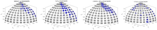
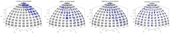
Figure 1.
Solutions with median IGD value among 30 runs obtained by NSGA-II, ToP, CMOEA_MS, CTAEA, CCMO, cDPEA, EMCMO, and CDCBM on DASCMOP9.
DOC [14] functions: The DOC test suite is very challenging, in which nine test functions involve both decision space and target space constraints. According to its complex characteristics, the CPF can be continuous, discrete, mixed, or degenerate. As seen from the experimental results of the eight algorithms in Table 4, CDCBM achieved the seven best test results out of nine problems. Figure 2 reflects the performance of each algorithm. NSGA-II [6] is too concerned with satisfying constraints and thus fell into a local optimum, failing to converge to the true PF. Because ToP [14] did not fully utilize the feasible solutions found in the first stage, it did not converge. C-TAEA [8] cannot cross the infeasible barrier, so that no feasible solution can be found. Neither the auxiliary populations of cDPEA [18] nor EMCMO [20] could provide better CPF information resulting in poor performance. CDCBM outperformed DOC2 because the main population fully used the information of the promising infeasible solutions of the auxiliary population, resulting in better distribution. CCMO [7] converged to the CPF, but in terms of distribution, CDCBM is slightly better than CCMO [6].
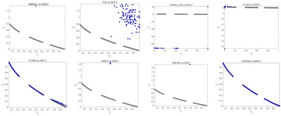
Figure 2.
Solutions with median IGD value among 30 runs obtained by NSGA-II, ToP, CMOEA_MS, CTAEA, CCMO, cDPEA, EMCMO, and CDCBM on DOC2.
LIRCMOP functions: Most of the test problems in LIRCMOP [26] problems contain many disjoint small feasible regions, hindered by extensive infeasible regions; the CPF usually consists of several disjoint segments or sparse points, and some CPFs even have just a curve. This poses severe challenges to maintaining population diversity. The experimental results in Table 4 show that CDCBM performed the best on 10 problems. EMCMO [20], cDPEA [18], and CMOEA_MS [5] achieved the best results on 2, 1, and 1 problem, respectively, while the other four algorithms did not achieve the best results on this test suite.
As shown in Figure 3, since the feasible region of LIRCMOP4 is only a discontinuous line segment, NSGA-II [6], ToP [14], CTAEA [8], CCMO [7], cDPEA [18], and EMCMO [20] all fall into local optima. However, only CDCBM found all discontinuous CPFs.
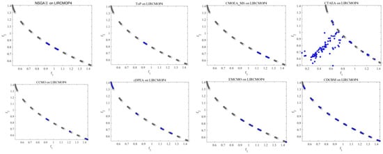
Figure 3.
Solutions with median IGD value among 30 runs obtained by NSGA-II, ToP, CMOEA_MS, CTAEA, CCMO, cDPEA, EMCMO, and CDCBM on LIRCMOP4.
Real-world CMOPs: The comparison of our algorithm with the comparative algorithm on three real-world problems is presented here. The Spring Design problem [30] has two optimization objectives, eight inequality constraints, and three decision variables. The synchronous optimal pulse width modulation of 3-level and 5-level inverter problem [31,32] has two optimization objectives, 24 inequality constraints, and 25 decision variables. The definitions of all optimization objectives and constraints can be found in their references. The HV results of our algorithm and the comparative algorithm are given in Table 5. From Table 5, we can see that our algorithm obtains the maximum HV on these three real-world problems, indicating that our algorithm achieves the best performance on these three problems.
Table 5.
The HV values obtained by CDCBM and seven compared algorithms on all three benchmark sets. The first figure is the mean HV values, and the standard deviation is in parentheses. “NAN” means that the algorithm did not find any feasible solution in 30 runs. ‘+’, ‘−’, and ‘=‘ indicate better, worse, or equivalent results than CDCBM. Values highlighted in grey represent the best results achieved in each test question.
3.3. Further Investigations of CDCBM
In this subsection, we discuss the impact of changes in the constraint bound on the algorithm, which compares CDCBM with two variants on the LIRCMOP benchmark suite. The first variant of CDCBM adopts a decreasing bound, and the second variant bounds value to infinity all the time during the evolution. These two variables verify that the dynamic constraint bounds are valid.
Table 6 presents the performance of CDCBM and its two variants on the LIRCMOP suite. We can see that CDCBM gets the eight best averages on LIRCMOP. Although Variant 1 and Variant 2 obtained five and one best averages, respectively, they did not show significant differences. Furthermore, CDCBM has five and seven results that significantly outperform Variant 1 and Variant 2, respectively, demonstrating the effectiveness of dynamically constrained boundaries.
Table 6.
The IGD values obtained by CDCBM and its two variants on the DASCMOP benchmark suite. The first figure is the mean IGD values, and the standard deviation is in parentheses. Best result in each row is highlighted.
4. Discussion
In this section, to demonstrate the effectiveness of our algorithm, we visualize the running process of seven algorithm, NSGA-II [6], ToP [14], CMOEA_MS [5], CTAEA [8], CCMO [7], cDPEA [18], EMCMO [20], and CDCBM. Figure 4 presents the population distribution of all seven CMOEAs on LIRCMOP3 at different generations.
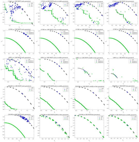
Figure 4.
Population distribution of five CMOEAs on LIRCMOP3 in different generations, where the grey line is CPF, and infeasible regions are represented by the white regions.
CTAEA: CTAEA [8] includes a Convergence Oriented Archive (CA) and a Diversity Oriented (DA). Most of the parents in this algorithm are from CA and DA, and DA does not consider any constraints to provide CA with information about feasible regions that it has not explored. Early CA considers both objective and constraint and can partially converge to the feasible region, but most infeasible solutions will still exist in the population. However, the limited mate selection scheme in the middle and late stages affected the evolutionary direction of CA, and most of the offspring were located between CPF and UPF. Therefore, the convergence and diversity of CA are relatively poor.
CCMO: Population 1 considers constraints in the early stages of evolution and quickly converges to the local CPF, while population 2 does not consider constraints at all and converges to UPF. In the middle and late stages, CCMO [7] can obtain a well-distributed population 2. However, population 2 cannot continuously provide effective information for population 1 and cannot help population 1 to jump out of the local optimum, resulting in poor distribution.
cDPEA: cDPEA has better distribution in the early stage, thanks to adopting a self-adaptive penalty function. Then, the main population converges to the local CPF, and the auxiliary population converges to the UPF. In the middle-to-later stage, the auxiliary population starts to search between CPF and UPF, and some individuals come to the vicinity of the feasible region. However, the diversity of the auxiliary population is too poor to help the main population effectively. Finally, the main population is still limited to part of the CPF.
EMCMO: In this algorithm, CMOP is modeled as a multi-task optimization problem, the first task considers both constraints and objectives (i.e., CPF), and the auxiliary task is to find a well-distributed UPF. Its early stage is the same as CCMO [7]. In the early-to-middle and middle-to-later generations, the second task can better converge to the UPF. Furthermore, the designed heuristic method finds valuable knowledge and carries out knowledge transfer. Nevertheless, the CPF of LIRCMOP3 is far away from the UPF, which reduces the effect of knowledge transfer. This also makes the distribution of the main tasks between the middle and late generation and the previous generation the same, and neither can jump out of the local optimal area.
CDCBM: In the early stage, P2 converges to the UPF regardless of constraints, and the generated descendants help P1 converge to the feasible region. In the early-to-middle generation, as the gradually decreases, P2 gradually comes to the boundary of the feasible region. In the process of searching from UPF to CPF, P2 retains many potential infeasible solutions. These solutions help P1 find most of the CPFs, but some CPFs are still ignored during evolution. Therefore, in the middle-to-later generation, increases to a (a constraint tolerance value that gradually decreases with the evolutionary algebra), and P2 returns to the feasible region boundary to repeat the search. In this process, we will also judge the success rate of the parent and the offspring to more effectively provide a complementary evolutionary direction for P1. In the final generation, P1 finds all feasible regions and has a relatively good distribution.
5. Conclusions
We have proposed a MOEA based on the dynamic constraint boundary method. The auxiliary population evolves to the UPF without initially considering the constraints, and as the constraint boundary decreases, the population moves closer to the feasible region. These potentially infeasible solutions can help the main population to overcome obstacles in the infeasible region. In addition, when the auxiliary population reaches the CPF, the constraint boundary changes again, and the population returns to search near the feasible region. This operation preserves some well-distributed infeasible solutions to help the main population find potential unsearched feasible regions. Moreover, in the evolution process, according to the state of the auxiliary population, the effective parent and child individuals will be selected to enter the next generation update, which can effectively reduce the waste of iteration times.
Although the proposed CDCBM performed well on these several test suites, several aspects must be investigated. If all initial solutions are feasible, ε always takes infinity. In this case, it is necessary to find a way to set an appropriate initial value because it has a relatively significant impact on the evolution of the auxiliary population. In addition, we will explore our algorithm parameters in more detail to better improve our algorithm.
Author Contributions
Conceptualization, Z.L.; methodology, Q.W.; software, Q.W.; validation, Z.L.; formal analysis, Z.L.; investigation, Z.L.; resources, J.Z.; writing—original draft preparation, Z.L.; writing—review and editing, Z.L.; visualization, Z.L.; supervision, X.Y.; project administration, Y.L., Y.H. and Y.X.; funding acquisition, Q.W. All authors have read and agreed to the published version of the manuscript.
Funding
The authors wish to thank the support of the National Natural Science Foundation of China (Grant No. 61876164), the Natural Science Foundation of Hunan Province (Grant No. 2022JJ40452), Doctoral research start-up project (Grant No. 22QDZ03).
Data Availability Statement
The data presented in this study are available on request from the corresponding author. The data are not publicly available due to the data provider’s request for confidentiality of the data and results.
Acknowledgments
We thank our institute teachers and students for their support in the work of this paper.
Conflicts of Interest
The authors declare no conflict of interest.
References
- Deb, K. Multi-Objective Optimization Using Evolutionary Algorithms; John Wiley & Sons: Chichester, UK, 2001. [Google Scholar]
- Wang, J.; Ren, W.; Zhang, Z.; Huang, H.; Zhou, Y. A hybrid multiobjective memetic algorithm for multiobjective periodic vehicle routing problem with time windows. IEEE Trans. Syst. Man. Cybern. Syst. 2020, 50, 4732–4745. [Google Scholar] [CrossRef]
- Tanabe, R.; Oyama, A. A note on constrained multi-objective optimization benchmark problems. In Proceedings of the IEEE Congress on Evolutionary Computation (CEC), Donostia, Spain, 5–8 June 2017; pp. 1127–1134. [Google Scholar]
- Ma, Z.; Wang, Y. Evolutionary constrained multiobjective optimization: Test suite construction and performance comparisons. IEEE Trans. Evol. Comput. 2019, 23, 972–986. [Google Scholar] [CrossRef]
- Tian, Y.; Zhang, Y.; Su, Y.; Zhang, X.; Tan, K.C.; Jin, Y. Balancing objective optimization and constraint satisfaction in constrained evolutionary multiobjective optimization. IEEE Trans. Cybern. 2021. [Google Scholar] [CrossRef] [PubMed]
- Deb, K.; Pratap, A.; Agarwal, S.; Meyarivan, T.A.M.T. A fast and elitist multiobjective genetic algorithm: NSGA-II. IEEE Trans. Evol. Comput. 2002, 6, 182–197. [Google Scholar] [CrossRef]
- Tian, Y.; Zhang, T.; Xiao, J.; Zhang, X.; Jin, Y. A coevolutionary framework for constrained multiobjective optimization problems. IEEE Trans. Evol. Comput. 2020, 25, 102–116. [Google Scholar] [CrossRef]
- Li, K.; Chen, R.; Fu, G.; Yao, X. Two-archive evolutionary algorithm for constrained multiobjective optimization. IEEE Trans. Evol. Comput. 2018, 23, 303–315. [Google Scholar] [CrossRef]
- Liang, J.; Ban, X.; Yu, K.; Qu, B.; Qiao, K.; Yue, C.; Chen, K.; Tan, K.C. A Survey on Evolutionary Constrained Multi-objective Optimization. IEEE Trans. Evol. Comput. 2022. [Google Scholar] [CrossRef]
- Ma, Z.; Wang, Y.; Song, W. A new fitness function with two rankings for evolutionary constrained multiobjective optimization. IEEE Trans. Syst. Man Cybern. Syst. 2019, 51, 5005–5016. [Google Scholar] [CrossRef]
- Zhang, Q.; Li, H. MOEA/D: A multiobjective evolutionary algorithm based on decomposition. IEEE Trans. Evol. Comput. 2007, 11, 712–731. [Google Scholar] [CrossRef]
- Fan, Z.; Li, W.; Cai, X.; Hu, K.; Lin, H.; Li, H. Angle-based constrained dominance principle in MOEA/D for constrained multi-objective optimization problems. In Proceedings of the 2016 IEEE Congress on Evolutionary Computation (CEC), Vancouver, BC, Canada, 24–29 July 2016; pp. 460–467. [Google Scholar]
- Fan, Z.; Li, W.; Cai, X.; Li, H.; Wei, C.; Zhang, Q.; Deb, K.; Goodman, E. Push and pull search for solving constrained multi-objective optimization problems. Swarm Evol. Comput. 2019, 44, 665–679. [Google Scholar] [CrossRef]
- Liu, Z.Z.; Wang, Y. Handling constrained multiobjective optimization problems with constraints in both the decision and objective spaces. IEEE Trans. Evol. Comput. 2019, 23, 870–884. [Google Scholar] [CrossRef]
- Ma, H.; Wei, H.; Tian, Y.; Cheng, R.; Zhang, X. A multi-stage evolutionary algorithm for multi-objective optimization with complex constraints. Inf. Sci. 2021, 560, 68–91. [Google Scholar] [CrossRef]
- Zhu, Q.; Zhang, Q.; Lin, Q. A constrained multiobjective evolutionary algorithm with detect-and-escape strategy. IEEE Trans. Evol. Comput. 2020, 24, 938–947. [Google Scholar] [CrossRef]
- Ming, M.; Wang, R.; Ishibuchi, H.; Zhang, T. A Novel Dual-Stage Dual-Population Evolutionary Algorithm for Constrained Multi-Objective Optimization. IEEE Trans. Evol. Comput. 2021, 26, 1129–1143. [Google Scholar] [CrossRef]
- Ming, M.; Trivedi, A.; Wang, R.; Srinivasan, D.; Zhang, T. A dual-population-based evolutionary algorithm for constrained multiobjective optimization. IEEE Trans. Evol. Comput. 2021, 25, 739–753. [Google Scholar] [CrossRef]
- Zou, J.; Sun, R.; Yang, S.; Zheng, J. A dual-population algorithm based on alternative evolution and degeneration for solving constrained multi-objective optimization problems. Inf. Sci. 2021, 579, 89–102. [Google Scholar] [CrossRef]
- Qiao, K.; Yu, K.; Qu, B.; Liang, J.; Song, H.; Yue, C. An evolutionary multitasking optimization framework for constrained multiobjective optimization problems. IEEE Trans. Evol. Comput. 2022, 26, 263–277. [Google Scholar] [CrossRef]
- Deb, K.; Agrawal, R.B. Simulated binary crossover for continuous search space. Complex Syst. 1995, 9, 115–148. [Google Scholar]
- Deb, K. An efficient constraint handling method for genetic algorithms. Comput. Methods Appl. Mech. Eng. 2000, 186, 311–338. [Google Scholar] [CrossRef]
- Das, S.; Suganthan, P.N. Differential evolution: A survey of the state-of-the-art. IEEE Trans. Evol. Comput. 2010, 15, 4–31. [Google Scholar] [CrossRef]
- Tian, Y.; Cheng, R.; Zhang, X.; Jin, Y. PlatEMO: A MATLAB platform for evolutionary multi-objective optimization [educational forum. IEEE Comput. Intell. Mag. 2017, 12, 73–87. [Google Scholar] [CrossRef]
- Fan, Z.; Li, W.; Cai, X.; Li, H.; Wei, C.; Zhang, Q.; Deb, K.; Goodman, E. Difficulty adjustable and scalable constrained multiobjective test problem toolkit. Evol. Comput. 2020, 28, 339–378. [Google Scholar] [CrossRef] [PubMed]
- Fan, Z.; Li, W.; Cai, X.; Huang, H.; Fang, Y.; You, Y.; Mo, J.; Wei, C.; Goodman, E. An improved epsilon constraint-handling method in MOEA/D for CMOPs with large infeasible regions. Soft Comput. 2019, 23, 12491–12510. [Google Scholar] [CrossRef]
- Bosman, P.A.N.; Thierens, D. The balance between proximity and diversity in multiobjective evolutionary algorithms. IEEE Trans. Evol. Comput. 2003, 7, 174–188. [Google Scholar] [CrossRef]
- While, L.; Hingston, P.; Barone, L.; Huband, S. A faster algorithm for calculating hypervolume. IEEE Trans. Evol. Comput. 2006, 10, 29–38. [Google Scholar] [CrossRef]
- Zitzler, E.; Knowles, J.; Thiele, L. Quality assessment of pareto set approximations. Multiobject. Optim. 2008, 52, 373–404. [Google Scholar]
- Kannan, B.; Kramer, S.N. An augmented lagrange multiplier based method for mixed integer iscrete continuous optimization and its applications to mechanical design. J. Mech. Des. 1994, 116, 405–411. [Google Scholar] [CrossRef]
- Rathore, A.; Holtz, J.; Boller, T. Optimal pulsewidth modulation of multilevel inverters for low switching frequency control of medium voltage high power industrial ac drives. In Proceedings of the 2010 IEEE Energy Conversion Congress and Exposition, Atlanta, GA, USA, 12–16 September 2010. [Google Scholar] [CrossRef]
- Rathore, A.; Holtz, J.; Boller, T. Synchronous optimal pulsewidth modulation for low-switching-frequency control of medium-voltage multilevel inverters. Ind. Electron. IEEE Trans. 2010, 57, 2374–2381. [Google Scholar] [CrossRef]
Publisher’s Note: MDPI stays neutral with regard to jurisdictional claims in published maps and institutional affiliations. |
© 2022 by the authors. Licensee MDPI, Basel, Switzerland. This article is an open access article distributed under the terms and conditions of the Creative Commons Attribution (CC BY) license (https://creativecommons.org/licenses/by/4.0/).