Abstract
In this work, we design a multi-category inverse design neural network to map ordered periodic structures to physical parameters. The neural network model consists of two parts, a classifier and Structure-Parameter-Mapping (SPM) subnets. The classifier is used to identify structures, and the SPM subnets are used to predict physical parameters for desired structures. We also present an extensible reciprocal-space data augmentation method to guarantee the rotation and translation invariant of periodic structures. We apply the proposed network model and data augmentation method to two-dimensional diblock copolymers based on the Landau–Brazovskii model. Results show that the multi-category inverse design neural network has high accuracy in predicting physical parameters for desired structures. Moreover, the idea of multi-categorization can also be extended to other inverse design problems.
Keywords:
inverse design; multi-category network; reciprocal-space data augmentation method; Landau-Brazovskii model; diblock copolymers; periodic structure MSC:
68T07; 35R30; 35Q68; 74E15; 03C64
1. Introduction
Material properties are mainly determined by microscopic structures. Therefore, to obtain satisfactory properties, how to find desired structures is very important in material design. The formation of ordered structures directly relies on physical conditions, such as temperature, pressure, molecular components, and geometry confinement. However, the relationship between ordered structures and physical conditions is extremely complicated and diversified. A traditional approach is a trial-and-error manner, i.e., passively finding ordered structures for given physical conditions. This approach, in terms of solving the direct problem, is time-consuming and expensive. A wise way is an inverse design that turns to find physical conditions for desired structures.
In this work, we are concerned about the theoretical development of the inverse design method for block copolymers. Block copolymer systems are important materials in industrial applications since they can self-assemble into innumerous ordered structures. There are many approaches for solving the direct problem of block copolymer systems, such as the first principle calculation [1], Monte Carlo simulation [2,3], molecular dynamics [4], dissipative particle dynamics [5,6], self-consistent field simulation [7], and density functional theory [8]. In the past decades, a directed self-assembly (DSA) method has been developed to invert design block copolymers. Liu et al. [9] presented an integration scheme of a block-copolymer-directed assembly with 193 nm immersion lithography, and provided a pattern quality that was comparable with existing double patterning techniques. Suh et al. [10] obtained nanopatterns via DSA of block copolymer films with a vapor-phase-deposited topcoat. Many DSA strategies have been also developed for the fabrication of ordered square patterns to satisfy the demand for lithography in semiconductors [11,12,13,14].
With the rise of data science and machine learning, many deep-learning inverse design methods have been developed to learn the mapping between structures and physical parameters [15,16,17,18]. These new techniques and methods are beginning to be used to study block copolymers. Yao et al. combined machine learning with self-consistent field theory (SCFT) to accelerate the exploration of parameter space for block copolymers [19]. Lin and Yu designed a deep learning solver inspired by physical-informed neural networks to tackle the inverse discovery of the interaction parameters and the embedded chemical potential fields for an observed structure [20]. Based on the idea of classifying first and fitting later, Katsumi et al. estimated Flory–Huggins interaction parameters of diblock copolymers from cross-sectional images of phase-separated structures [21]. The phase diagrams of block copolymers could be predicted by combining the deep learning technique and SCFT [22,23].
In this work, we propose a new neural network to address inverse design problem based on the idea of multi-categorization. We take the AB diblock copolymer system as an example to demonstrate the performance of our network. The training and test datasets are generated from the Landau–Brazovskii (LB) model [24]. The LB model is an effective tool to describe the phases and phase transition of diblock copolymers [25,26,27,28,29]. Let be the order parameter, a function of spatial position , which represents the density distribution of diblock copolymers. The free energy functional of the LB model is
where satisfies the mass conservation and is the system volume. The model parameters in (1) are associated to physical conditions of diblock copolymers. Concretely, is a temperature-like parameter related to the Flory–Huggins interaction parameter, the degree of polymerization N, and the A monomer fraction f of each diblock copolymer chain. can control the onset of the order–disorder spinodal decomposition. The disordered phase becomes unstable at . is associated with f and N; it is nonzero only if the AB diblock copolymers chain is asymmetric. is the bare correlation length. Further relationships can be found in [25,26,27,28,29]. The stationary states of the LB free energy functional correspond to ordered structures.
The rest of the paper is organized as follows. In Section 2, we solve the LB model (1) to obtain datasets. In Section 3, we present the multi-category inverse design neural network and the reciprocal-space data augmentation method for periodic structures. In Section 4, we take the diblock copolymer system confined in two dimensions as an example to test the performance of our proposed inverse design neural network model. In Section 5, we draw a brief summary of this work.
2. Direct Problem
Solving the direct problem involves optimizing the LB free energy functional (1) to obtain stationary states corresponding to ordered structures:
Here, we only consider periodic structures. Therefore, we can apply the Fourier pseudospectral method to discretize the above optimization problem.
2.1. Fourier Pseudospectral Method
For a periodic order parameter , , where is the primitive Bravis lattice. The primitive reciprocal lattice , satisfying the dual relationship
The order parameter can be expanded as
where the Fourier coefficient
is the volume of .
We define the discrete grid set as
where the number of elements of is . Denote the grid periodic function space = {, f is periodic}. For any periodic grid functions , the -inner product is defined as
The discrete reciprocal space is
and the discrete Fourier coefficients of in can be represented as
For and , we have the discrete orthogonality
Therefore, the discrete Fourier transform of is
The -order trigonometric polynomial is
Then, for , we have .
Due to the orthogonality (10), the LB energy functional can be discretized as
where , , and . The convolutions in the above expression can be efficiently calculated through the fast Fourier transform (FFT). Moreover, the mass conservation constraint is discretized as
where . Therefore, (2) reduces to a finite dimensional optimization problem
where and are the discretized interaction and bulk energies
In the work, we employ the adaptive APG method to solve (15).
2.2. Phase Diagram
Given parameters , we can obtain the stationary states by solving the free energy functional . Due to the non-convexity of LB free energy functional, there are many, even infinite stationary states for given parameters. We need to determine the stationary state with the lowest energy, which corresponds to the most probable ordered structure observed in experiments. It requires comparing the energies of stationary states to obtain the stable structure and constructing a phase diagram. In the following, we consider disordered (DIS), cylindrical hexagonal (HEX), lamellar (LAM), body-centered cubic (BCC), and double gyroid (DG) phases as candidate structures. We use the AGPD software [30] to produce a -plane phase diagram, as shown in Figure 1. The obtained phase diagram is consistent with previous work [29,31,32].
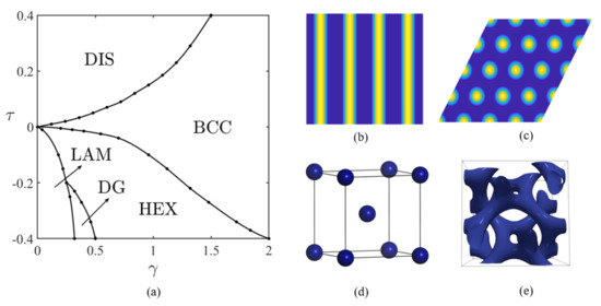
Figure 1.
(a) Phase diagram of the Landau-Brazovskii model. (b) LAM. (c) HEX. (d) BCC. (e) DG.
3. Inverse Design Neural Network
3.1. Multi-Category Inverse Design Network
The architecture of the multi-category inverse design network for predicting physical parameters for the desired periodic structure is shown in Figure 2. The neural network mainly consists of two modules: a classifier and SPM subnets. The former (orange block) identifies and classifies candidate structures, and the latter (blue block) including a family of subnets is a mapping connecting physical parameters and ordered structures.

Figure 2.
Multi-category inverse design network.
According to the characteristics of the problem, we can design corresponding network architectures of classifier and SPM subnets. In this work, the classifier and each SPM subnet use the same network architecture as shown in Figure 3. Concretely, the network contains an input layer, three convolutional layers, three max-pooling layers, four fully connected layers, and an output layer. For the classifier network, the size of the output layer represents the number of categories, while for each subnet, it means the number of predicted physical parameters. The network architecture is a development of the Lenet-5 network [33].

Figure 3.
Network architecture of classifier and each SPM subnet.
3.2. Computational Complexity
In this subsection, we analyze the computational complexity of the network architecture of the classifier and each SPM subnet. As shown in Figure 3, the network consists of three parts:
- Convolution. The computational amount of a convolution layer is , where is the size of the convolution kernel. and represent the number of channels of the previous layer and the current layer. H and W are the height and width of the current layer.
- Max-pooling. The computational amount of a pooling layer is , where is the size of the pooling kernel. and represent the number of channels of the previous layer and the current layer. H and W are the height and width of the current layer.
- Full connection. The computational amount of a fully connected layer is , where and represent the dimensionality of the previous layer and the current layer.
3.3. Reciprocal-Space Data Augmentation (RSDA) Method
Generally, the ability of a network depends not only on its architecture, but also on the amount and properties of data. Due to the rotation and translation invariance of periodic structures, how to make the classifier recognize the invariance is very important. Here, we use a data augmentation method to increase the amount of data. Existing data augmentation methods, such as Swapping, Mixup, Insertion, and Substitution, are often used for classification tasks, see a recent review [34] and the references therein. However, as the dataset increases, these data augmentation approaches might become expensive, and it would be easy to use the wrong labels to train the network. For one-dimensional periodic phases, Yao et al. [19] used a Period-Filling method for data augmentation. However, this approach is difficult to extend to higher dimensions.
In this paper, we propose an extensible data augmentation method implemented in reciprocal space called the RSDA method. For a periodic structure, the primary wave vectors in the reciprocal space can describe the main features of the structure. The RSDA method uses the information of the primary wave vectors for data augmentation. We denote the fundamental domain of periodic structure as . For any translation , ; therefore, we only need to consider the translation in the fundamental domain . From the Fourier expansion , and for rotation matrix , , we have
where is a new reciprocal lattice by rotation transformation and is a new Fourier coefficient associated with translation transformation. Obviously, the RSDA method is easy to implement, and can be suitable for arbitrary dimensional periodic structures.
4. Application
In this section, we apply the multi-category network model to diblock copolymers confined on a two-dimensional plane to obtain the mapping from periodic structure to physical parameters. Besides, we compare the approximation accuracy and computational time of forecasting parameters. All the experiments in this section are conducted on a workstation equipped with two Intel(R) Xeon(R) Silver 4214 CPUs @ 2.20 GHz with 128 GB RAM. As the phase diagram shows, in two dimensions, only LAM and HEX phases are thermodynamic stable. Therefore, the SPM has two subnets, i.e., LAM and HEX subnets. As shown in Figure 4, the classifier is used to distinguish LAM or HEX phase after inputting the order parameter . For desired structures, LAM and HEX subnets are used to predict the physical parameters . The dataset required for the classifier consists of , where is the label, and for each SPM subnet, consists of ; N is the size of training data.

Figure 4.
Network of the two-dimensional diblock copolymer system.
Table 1 shows the network parameters of the classifier and SPM subnets. In all networks, the size of the output layer is 2. We adopt the ReLU function as the activation function and the Adam optimizer with a learning rate of to train the neural network model. Kaiming_uniform [35] is used to initialize the network parameters both in tje classifier and subnets. We set the maximum epoch to be 20,000 and stop training if the error on the validation set decreases to to prevent overfitting. For the classifier, the loss function is defined as
where represents the label of the sample, LAM phase is 0, and HEX phase is 1. is the probability of identifying HEX phase. For each SPM subnet, the loss function is
where are the targeted parameters and are the predicted parameters.

Table 1.
Network parameters of classifier and each subnet. The notations of parameters in the table are as follows: in channels (i), out channels (o), kernel size (k), stride (s), padding (p), batch size (Nb).
It is well known that the LAM and HEX phases have 2- and 6-fold symmetries, respectively. As shown in Figure 5a,b, the fundamental domain of the LAM phase is a square, while the fundamental domain of the HEX phase is a parallelogram region due to the 6-fold rotational symmetry. Their corresponding primitive Bravis lattice is
Lattice constants and depend on the model parameters.

Figure 5.
Schematic diagram of fundamental domain. (a) LAM phase ; (b) HEX phase . Illustration of rotating primary spectral points of (c) LAM and (d) HEX phases in reciprocal space. Reference state (red); transform state after rotating degree(s) (blue).
Now, we construct the dataset of the LAM phase. We discrete the - phase space of the stable LAM phase with step size to form the dataset for training and validation, and with step size to form for testing. We randomly choose 627 parameter pairs as a group from to construct training and validation sets, and 262 parameter pairs as a group from to build the test set. Then, we generate LAM phases by solving the direct problem with each selected parameter pair in and .
We augment data by rotation and translation. The rotation matrix is
where is the rotation angle. LAM phases have 2-fold rotational symmetry; therefore, . Figure 5c gives a sketch plot of rotating LAM phase in the reciprocal space. Concretely, we rotate 627 LAM phases in with and translate them with . The dataset we obtained includes 188,100 LAM phases. We randomly split these samples into a training set and a validation set at a ratio of 4:1. In the group , 262 LAM phases are rotated by , 7°, 19°, 20°, 27°, 34°, 78°, 80°, 82°, and translated by , , , , to form the test set.
Similarly, we construct a dataset of the HEX phase. The - domain of the stable HEX phase is discretized with step size to form for training and validation, and with step size to form for testing. We randomly choose 1600 parameter pairs as a group from to construct training and validation sets, and 300 parameter pairs as a group from to build the test set. We still obtain HEX phases by solving the direct problem for selected parameters.
Then, we augment the dataset by rotation and translation operators. The HEX phase has 6-fold rotational symmetry; therefore, the rotation angle in (20) belongs to . An illustration of rotating HEX phase in the reciprocal space is shown in Figure 5d. Concretely, we discretize rotation angle and select translation vector in , , for processing each sample in . This results in 16,000 HEX phases. We randomly divide them into a training set and a validation set with a ratio of 4:1. The generated dataset of 300 in is rotated by , 11°, 24°, 27°, 38°, 40°, 52°, 54°, and translated by , , , , , to form the test set.
Some LAM and HEX phases under rotation and translation transformation are visually illustrated in Figure 6. The sizes of training, validation, and test sets for the classifier are given in Table 2.
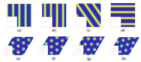
Figure 6.
Density and spectral pattern of LAM and HEX phases under rotation and translation transformation. LAM phases at : (a) = 0, ; (b) = 0, ; (c) = , ; (d) = , . HEX phases : (e) = 0, ; (f) = 0, ; (g) = , ; (h) = , .

Table 2.
Amount of training, validation, and test data for the classifier.
Figure 7 shows the training and validation loss of the classifier. One can find that the training and validation losses reach and at epoch = 5, respectively. The accuracy is defined as , where is the confusion matrix [21]—a visual table layout that reflects the predictions of the network. As shown in Table 3, denotes the number of i identified to be j, and . These results show that the classifier can identify structures with 100% success.
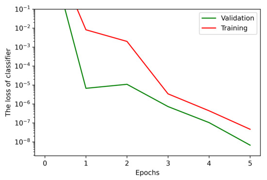
Figure 7.
Training and validation losses of classifier.

Table 3.
The confusion matrix of classifier at epoch = 5.
We classify the training and validation data by the classifier and obtain 188,100 LAM and 160,000 HEX phases. Then, we adopt them as the training and validation data for each subnet. For the test data onto each subnet, we only consider the data translated by in the test set. Table 4 indicates the size of the dataset for each SPM subnet.

Table 4.
Amount of training, validation, and test data for LAM and HEX subnets.
Figure 8 presents the training and validation losses of SPM networks. We can see that the training loss of the LAM (HEX) subnet is () and the validation loss is () at epoch = 700 (1200).
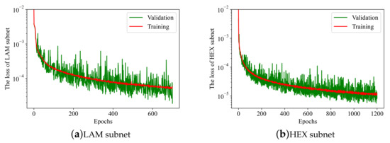
Figure 8.
The training and validation losses of SPM subnets: (a) LAM and (b) HEX.
We define the relative error
and the average relative error
where is the size of test data. The predicted accuracy of single sample is , while the average accuracy is . Figure 9 illustrates the test accuracy of the LAM and HEX subnets. Results indicate that the accuracy of parameters prediction for a single sample can achieve , and the average prediction accuracy of LAM subnet (blue dashed line) is 84%. For the HEX subnet (pink dashed line), the average prediction accuracy can reach 91%.
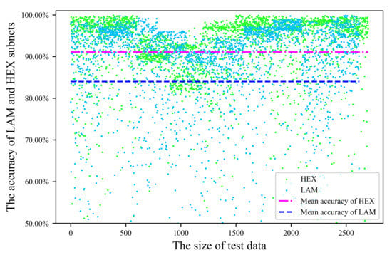
Figure 9.
The test accuracy of LAM (blue) and HEX (green) subnets. Scatter plots demonstrate the parameter prediction accuracy of HEX and LAM subnets. The average test accuracy of the two subnets is shown by two dashed lines.
We randomly select two test samples in the test set and input them into the network to predict the corresponding parameters. Next, we obtain structures corresponding to the predicted parameters by solving the direct problem. Figure 10 shows LAM and HEX phases with targeted and predicted parameters, and the absolute errors between the targeted and predicted phases. From Figure 10c,f, we can see that the absolute error of the LAM phase is and of the HEX phase is . This also reflects a good fitting effect of SPM subnets.
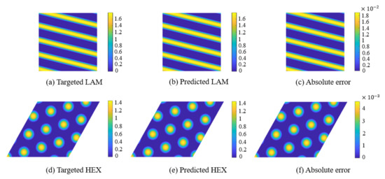
Figure 10.
The phases with targeted and predicted parameters are obtained by solving the direct problem (15). LAM phase: (a) [,] = [−0.4, 0.2], and ; (b) [,] = [−0.3914, 0.2067], and . HEX phase: (d) [,] = [−0.08, 0.28], and ; (e) [,] = [−0.0807, 0.2744], and . Absolute errors between targeted and predicted LAM (c) and HEX (f) phases.
Table 5 shows the training time of the classifier and each SPM subnet, and the online calculation time of these networks when identifying structures or predicting parameters with one sample in the test set.

Table 5.
Training and test time for the classifier and each SPM subnet.
5. Conclusions
In this paper, we propose a multi-category neural network for the inverse design of ordered periodic structures. The proposed network can construct the mapping between phases and physical parameters. For periodic phases, we provide an extensible RSDA approach to augment data. Then, we apply these methods to the two-dimensional diblock copolymer system. The dataset is produced by the LB free energy functional. Experimental results show that the structure recognition accuracy of the classifier can reach 100% based on 26,600 randomly selected test data. Moreover, on a dataset consisting of 5320 randomly selected test data, the parameter prediction accuracy of the LAM phase reaches 84% and the accuracy of the HEX phase reaches 91%. The network model and RSDA method are applied to a two-dimensional problem; however, they can be extended to higher-dimensional inverse design problems.
Author Contributions
Conceptualization, Y.H., K.J., D.W. and T.Z.; methodology, Y.H., K.J., D.W. and T.Z.; software, D.W. and T.Z.; validation, K.J., D.W. and T.Z.; formal analysis, K.J., D.W. and T.Z.; investigation, K.J., D.W. and T.Z.; resources, K.J., D.W. and T.Z.; data curation, D.W. and T.Z.; writing—original draft preparation, K.J., D.W. and T.Z.; writing—review and editing, K.J., D.W. and T.Z.; visualization, K.J., D.W. and T.Z.; supervision, Y.H. and K.J. All authors have read and agreed to the published version of the manuscript.
Funding
This research was funded by NSFC Project (12171412, 11971410). K.J. is partially supported by the Natural Science Foundation for Distinguished Young Scholars of Hunan Province (2021JJ10037). Y.H. is partially supported by China’s National Key R&D Programs (2020YFA0713500).
Institutional Review Board Statement
Not applicable.
Informed Consent Statement
Not applicable.
Data Availability Statement
Not applicable.
Acknowledgments
The authors would like to thank Chen Cui and Liwei Tan for useful discussion.
Conflicts of Interest
The authors declare no conflict of interest.
References
- Beu, T.A.; Onoe, J.; Hida, A. First-principles calculations of the electronic structure of one-dimensional C60 polymers. Phys. Rev. B 2005, 72, 155416. [Google Scholar] [CrossRef]
- He, X.; Song, M.; Liang, H.; Pan, C. Self-assembly of the symmetric diblock copolymer in a confined state: Monte Carlo simulation. J. Chem. Phys. 2001, 114, 10510–10513. [Google Scholar] [CrossRef]
- Sugimura, N.; Ohno, K. A Monte Carlo simulation of water + oil + ABA block copolymer ternary system. I. Patterns in thermal equilibrium. AIP Adv. 2021, 11, 055312. [Google Scholar] [CrossRef]
- Lemak, A.S.; Lepock, J.R.; Chen, J.Z. Molecular dynamics simulations of a protein model in uniform and elongational flows. Proteins Struct. Funct. Bioinform. 2003, 51, 224–235. [Google Scholar] [CrossRef] [PubMed]
- Ortiz, V.; Nielsen, S.O.; Discher, D.E.; Klein, M.L.; Lipowsky, R.; Shillcock, J. Dissipative particle dynamics simulations of polymersomes. J. Phys. Chem. B 2005, 109, 17708–17714. [Google Scholar] [CrossRef][Green Version]
- Gavrilov, A.A.; Kudryavtsev, Y.V.; Chertovich, A.V. Phase diagrams of block copolymer melts by dissipative particle dynamics simulations. J. Chem. Phys. 2013, 139, 224901. [Google Scholar] [CrossRef]
- Fredrickson, G.; Fredrickson, D. The Equilibrium Theory of Inhomogeneous Polymers; International Series of Monographs on Physics; OUP Oxford: Oxford, UK, 2006. [Google Scholar]
- Fraaije, J. Dynamic density functional theory for microphase separation kinetics of block copolymer melts. J. Chem. Phys. 1993, 99, 9202–9212. [Google Scholar] [CrossRef]
- Liu, C.C.; Nealey, P.F.; Raub, A.K.; Hakeem, P.J.; Brueck, S.R.J.; Han, E.; Gopalan, P. Integration of block copolymer directed assembly with 193 immersion lithography. J. Vac. Sci. Technol. B 2010, 28, C6B30. [Google Scholar] [CrossRef]
- Suh, H.S.; Kim, D.H.; Moni, P.; Xiong, S.; Ocola, L.E.; Zaluzec, N.J.; Gleason, K.K.; Nealey, P.F. Sub-10-nm patterning via directed self-assembly of block copolymer films with a vapour-phase deposited topcoat. Nat. Nanotechnol. 2017, 12, 575–581. [Google Scholar] [CrossRef]
- Li, W.; Gu, X. Square patterns formed from the directed self-assembly of block copolymers. Mol. Syst. Des. Eng. 2021, 6, 355–367. [Google Scholar] [CrossRef]
- Ouk Kim, S.; Solak, H.H.; Stoykovich, M.P.; Ferrier, N.J.; De Pablo, J.J.; Nealey, P.F. Epitaxial self-assembly of block copolymers on lithographically defined nanopatterned substrates. Nature 2003, 424, 411–414. [Google Scholar] [CrossRef] [PubMed]
- Ji, S.; Nagpal, U.; Liao, W.; Liu, C.C.; de Pablo, J.J.; Nealey, P.F. Three-dimensional directed assembly of block copolymers together with two-dimensional square and rectangular nanolithography. Adv. Mater. 2011, 23, 3692–3697. [Google Scholar] [CrossRef] [PubMed]
- Chuang, V.P.; Gwyther, J.; Mickiewicz, R.A.; Manners, I.; Ross, C.A. Templated self-assembly of square symmetry arrays from an ABC triblock terpolymer. Nano Lett. 2009, 9, 4364–4369. [Google Scholar] [CrossRef]
- Malkiel, I.; Nagler, A.; Mrejen, M.; Arieli, U.; Wolf, L.; Suchowski, H. Deep learning for design and retrieval of nano-photonic structures. arXiv 2017, arXiv:1702.07949. [Google Scholar]
- Gahlmann, T.; Tassin, P. Deep neural networks for the prediction of the optical properties and the free-form inverse design of metamaterials. arXiv 2022, arXiv:2201.10387. [Google Scholar] [CrossRef]
- Liu, D.; Tan, Y.; Khoram, E.; Yu, Z. Training deep neural networks for the inverse design of nanophotonic structures. ACS Photonics 2018, 5, 1365–1369. [Google Scholar] [CrossRef]
- Peurifoy, J.; Shen, Y.; Jing, L.; Yang, Y.; Cano-Renteria, F.; DeLacy, B.G.; Tegmark, M.; Joannopoulos, J.D.; Soljacic, M. Nanophotonic particle simulation and inverse design using artificial neural networks. Sci. Adv. 2018, 4, eaar4206. [Google Scholar] [CrossRef] [PubMed]
- Xuan, Y.; Delaney, K.T.; Ceniceros, H.D.; Fredrickson, G.H. Deep learning and self-consistent field theory: A path towards accelerating polymer phase discovery. J. Comput. Phys. 2021, 443, 110519. [Google Scholar] [CrossRef]
- Lin, D.; Yu, H.Y. Deep learning and inverse discovery of polymer self-consistent field theory inspired by physics-informed neural networks. Phys. Rev. E 2022, 106, 014503. [Google Scholar] [CrossRef]
- Hagita, K.; Aoyagi, T.; Abe, Y.; Genda, S.; Honda, T. Deep learning-based estimation of Flory–Huggins parameter of A–B block copolymers from cross-sectional images of phase-separated structures. Sci. Rep. 2021, 11, 1–16. [Google Scholar] [CrossRef]
- Nakamura, I. Phase diagrams of polymer-containing liquid mixtures with a theory-embedded neural network. New J. Phys. 2020, 22, 015001. [Google Scholar] [CrossRef]
- Aoyagi, T. Deep learning model for predicting phase diagrams of block copolymers. Comput. Mater. Sci. 2021, 188, 110224. [Google Scholar] [CrossRef]
- Brazovskiĭ, S.A. Phase transition of an isotropic system to a nonuniform state. J. Exp. Theor. Phys. 1975, 41, 85–89. [Google Scholar]
- Leibler, L. Theory of microphase separation in block copolymers. Macromolecules 1980, 13, 1602–1617. [Google Scholar] [CrossRef]
- Fredrickson, G.; Helfand, E. Fluctuation effects in the theory of microphase separation in block copolymers. J. Chem. Phys. 1987, 87, 697. [Google Scholar] [CrossRef]
- Shi, A.C.; Noolandi, J.; Desai, R.C. Theory of anisotropic fluctuations in ordered block copolymer phases. Macromolecules 1996, 29, 6487–6504. [Google Scholar] [CrossRef]
- Miao, B.; Wickham, R.A. Fluctuation effects and the stability of the Fddd network phase in diblock copolymer melts. J. Chem. Phys. 2008, 128, 054902. [Google Scholar] [CrossRef]
- McClenagan, D. Landau Theory of Complex Ordered Phases. Ph.D. Thesis, McMaster University, Hamilton, ON, Canada, 2019. [Google Scholar]
- Jiang, K.; Si, W. AGPD: Automatically Generating Phase Diagram; National Copyright Administration: Beijing, China, 2022. [Google Scholar]
- Shi, A.C. Nature of anisotropic fluctuation modes in ordered systems. J. Phys. Condens. Matter 1999, 11, 10183–10197. [Google Scholar] [CrossRef]
- Zhang, P.; Zhang, X. An efficient numerical method of Landau–Brazovskii model. J. Comput. Phys. 2008, 227, 5859–5870. [Google Scholar] [CrossRef]
- LeCun, Y.; Bottou, L.; Bengio, Y.; Haffner, P. Gradient-based learning applied to document recognition. Proc. IEEE 1998, 86, 2278–2324. [Google Scholar] [CrossRef]
- Li, B.; Hou, Y.; Che, W. Data augmentation approaches in natural language processing: A survey. AI Open 2021, 3, 71–90. [Google Scholar] [CrossRef]
- He, K.; Zhang, X.; Ren, S.; Sun, J. Delving deep into rectifiers: Surpassing human-level performance on imagenet classification. In Proceedings of the IEEE International Conference on Computer Vision, Santiago, Chile, 7–13 December 2015; pp. 1026–1034. [Google Scholar]
Publisher’s Note: MDPI stays neutral with regard to jurisdictional claims in published maps and institutional affiliations. |
© 2022 by the authors. Licensee MDPI, Basel, Switzerland. This article is an open access article distributed under the terms and conditions of the Creative Commons Attribution (CC BY) license (https://creativecommons.org/licenses/by/4.0/).