A Many-Objective Evolutionary Algorithm Based on Indicator and Decomposition

Abstract

In the field of many-objective evolutionary optimization algorithms (MaOEAs), how to maintain the balance between convergence and diversity has been a significant research problem. With the increase of the number of objectives, the number of mutually nondominated solutions increases rapidly, and multi-objective evolutionary optimization algorithms, based on Pareto-dominated relations, become invalid because of the loss of selection pressure in environmental selection. In order to solve this problem, indicator-based many-objective evolutionary algorithms have been proposed; however, they are not good enough at maintaining diversity. Decomposition-based methods have achieved promising performance in keeping diversity. In this paper, we propose a MaOEA based on indicator and decomposition (IDEA) to keep the convergence and diversity simultaneously. Moreover, decomposition-based algorithms do not work well on irregular PFs. To tackle this problem, this paper develops a reference-points adjustment method based on the learning population. Experimental studies of several well-known benchmark problems show that IDEA is very effective compared to ten state-of-the-art many-objective algorithms.

1. Introduction

Mathematically, we define multiobjective optimization problems (MOPs) as [1]:

$$\left\{\begin{array}{c}minF\left(X\right)=(f_1\left(X\right),f_2\left(X\right),\dots ,f_m\left(X\right)),\hfill \\ subjecttoX\in \Omega .\hfill \end{array}\right.$$

(1)

where $X=(x_1,x_2,\dots ,x_n)$ is an n-dimensional decision variable vector in the decision space $\Omega$; $F\left(X\right)$ is an objective function vector that is composed of m conflicting objective functions.

For multi-objective optimization, it is expected to find a set of trade-off solutions for MOPs, called Pareto optimal solutions. Let $X_1$, $X_2$$\in \Omega$; $X_1$ is said to dominate $X_2$, denoted by $X_1\prec X_2$, if and only if $f_i\left(X_1\right)\le f_i\left(X_2\right)$ for each $i\in \{1,\dots ,m\}$ and $f_j\left(X_1\right)<f_j\left(X_2\right)$ for at least one index $j\in \{1,\dots ,m\}$; if none of X in $\Omega$ can dominate $X_1$, we call $X_1$ a nondominated or Pareto optimal solution. We call the set of all Pareto optimal solution points a Pareto set (PS), and call the set of all the Pareto optimal objective vector a Pareto optimal front (PF).

In recent years, with the development of multi-objective evolutionary optimization algorithms, a large number of algorithms have been proposed and made progress [2,3,4]. The MOPs with more than three objectives (i.e., m > 3) are called many-objective optimization problems (MaOPs) [5,6,7]. However, in MaOPs, with the increase of the number of objectives, most of the evolving individuals become mutually nondominated, so that the algorithms lose selection pressure [8]. To address this problem, researchers have proposed improved methods. The existing MaOEAs fall roughly into three categories: modified dominance-based, indicator-based and decomposition-based methods [6].

The first category is the modified dominance-based algorithms. These revise the dominance relationship to distinguish and select elite individuals. There are many techniques for developing new dominance relations, such as expanding the dominance area, gridding the objective space, and adopting fuzzy logic. ε-dominance [9], by introducing the parameter $\epsilon$ that extends the individual’s Pareto-dominated region, makes non-dominant individuals distinguishable. The Grid-dominance [10] distinguishes individuals by dividing the objective space into multiple grids. In order to further improve the search ability of the algorithm, a series of work has been proposed, such as Rotated-grid [11], RP-dominance [12], θ-dominance [13], fuzzy-based Pareto dominance [14] and rank-dominance [15]. They have been proved to be more effective than the traditional Pareto-dominance-based algorithms in terms of convergence.

The second category is indicator-based algorithms that use the indicator value of each individual as the selection criterion in environment selection. Many MaOEA performance indicators have been developed by researchers over the past few years, such as the hypervolume $HV$ [16], inverted GD ($IGD$) [17] and $I_{\infty }^r$ [18]. Although, as the number of objectives m increases, the computation time of the HV-based methods increases dramatically [19], but due to their good theoretical and Pareto compatible properties, they are very effective for solving MaOPs. The representative methods include HyPE [20] and MO-CMA-ES [21]. The IGD-like indicators such as $GD$, $IGD$ and $IG{D}^{+}$ estimate the distance between a population and the true PF. Specifically, Tian et al. [22] propose an adaptive reference-set method, $I_{{\epsilon }^{+}}$ indicator measures how far the PF is from the solution population, the IBEA [23] provides a general framework for indicator-based approaches and Yuan et al. propose a ratio-based indicator. These algorithms are challenging to evaluate the individual quality by building a subset of the true PF [19]. Although they perform well in convergence, the population diversity tends to be poor.

The third category is based on decomposition, which achieves the final effect by decomposing the MaOP into multiple single-objective subproblems and optimizing the subproblems simultaneously. MOEA/D [24] is a typical algorithm that decomposes a many-objective optimization problem into a set of sub-problems, and then optimizes the whole problem through the cooperation of neighbor sub-problems. There are many classic algorithms with similar ideal, such as NSGA-III [25], MOEA/DD [26], RVEA [27], and so on [28,29,30,31]. They have achieved promising performance on MaOPs with regular PFs, but some of them are not work well on irregular PFs [32,33]. To tackle this issue, reference-point-adjustment methods have been proposed, for instance, MOEA/D-AWA [34], NSGA-III [35], RVEA* [27], BCE [33], and so on [36,37,38,39]. In addition, there are algorithms [40,41] that are designed for specific problems and have excellent performance on specific problems. However, decomposition-only methods do not work well for problems with regular PFs.

The Pareto dominance sometimes fails due to over-reliance on maintaining diversity. Indicator-based methods can distinguish individuals in MaOPs, but they are poor in maintaining diversity [19]. In this paper, indicator-based and decomposition-based mechanisms are integrated into an algorithm, and IDEA is proposed. We use the $I_{\infty }^r$ [18] indicator to achieve population convergence and distinguish individuals, and employ the decomposition-based method to ensure population diversity. The contributions of this paper are summarized as follows:

1.

We use the $I_{\infty }^r$ indicator to achieve population convergence in the early stage so that the population can obtain the approximate PF. The maintenance of diversity is made for the obtained population through uniformly generated reference points, which make the final population possess good diversity.

2.

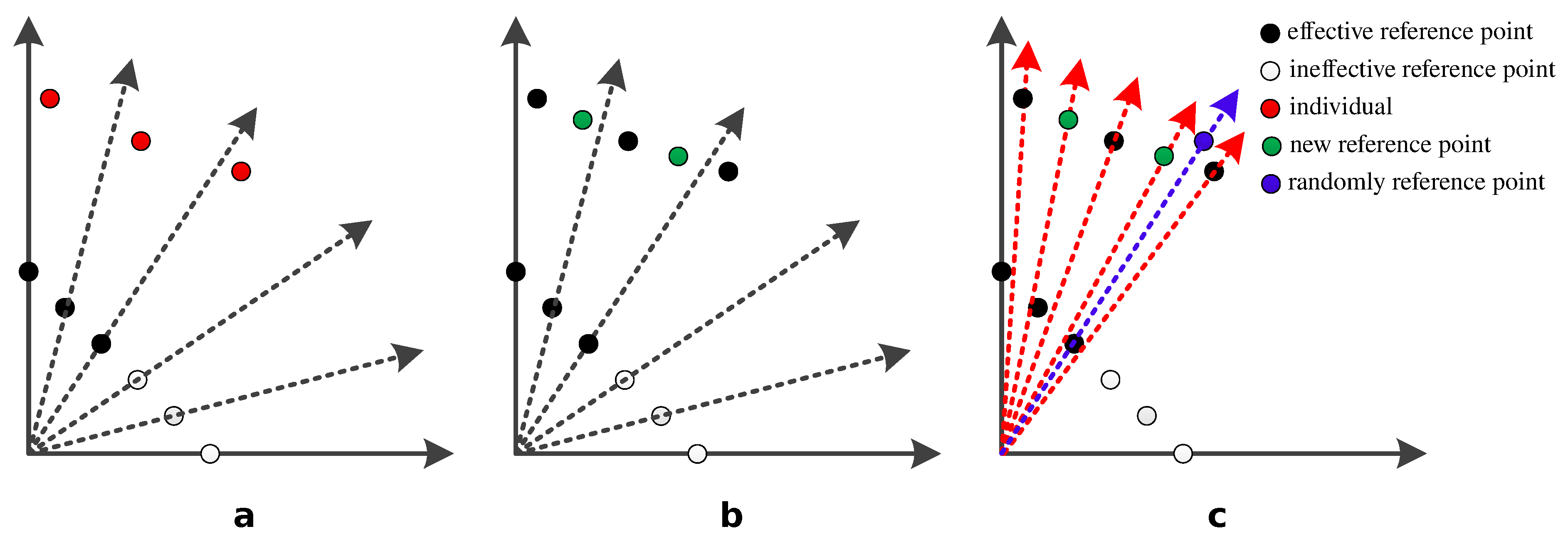
We propose an adaptive reference-point adjustment strategy based on the learning population for irregular PFs. A new reference-point set is generated through learning the population selected by the environment, and then the newly generated reference point set is used to select individuals for the next evolution.

3.

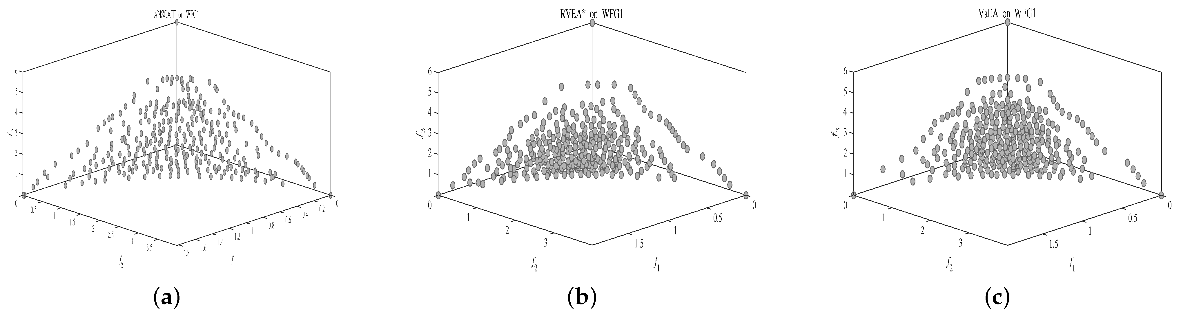
In order to maintain the diversity of the final solutions, we introduce a diversity-maintenance mechanism based on the vertical distance to the normal vector. Compared with other methods, this method is good at sharp tail PF shapes. Simulation experiments are carried out to verify the effectiveness of the proposed algorithm.

The rest of this article is organized as follows. Section 2 provides the background to this work. Section 3 covers the details of IDEA. Section 4 presents and analyzes a series of experiments. Finally, Section 5 summarizes this paper.

2. Preliminaries

In this section, the PREA algorithm is briefly introduced firstly, and then the penalty boundary intersection (PBI) [24] method is presented. Finally, the motivation of this paper is discussed.

2.1. $I_{\infty }^r$ Indicator

Let x, y$\in R_{+}^m$, the ratio-based-indicator value is defined as follows:

$$I_{\infty }^r\left(x\right|y)=\left\{\begin{array}{c}{\parallel \mathbb{R}(x,y)\parallel }_p,if\exists x_i>y_i;\hfill \\ -{\parallel \mathbb{R}(x,y)\parallel }_p,otherwise.\hfill \end{array}\right.$$

(2)

where $\mathbb{R}(x,y)$ = (max(0,$\frac{y_i}{x_i}-1$), …, max(0,$\frac{y_m}{x_m}-1$)) and ${\parallel \ast \parallel }_p$ stands for ${\ell }_p$-norm. $I_{\infty }^r\left(x\right|y)$ > $I_{\infty }^r\left(y\right|x)$ means x is better than y under this indicator. In PREA [18], the author proves that $I_{\infty }^r$ is a good form for eliminating outliers and protecting the PFs boundary points, and show that if this indicator value of an individual is greater than or equal to 0, the individual is a sufficient and necessary condition for the nondominated solution of the current population. The larger the indicator value is, the more important $x_i$ is in the current population.

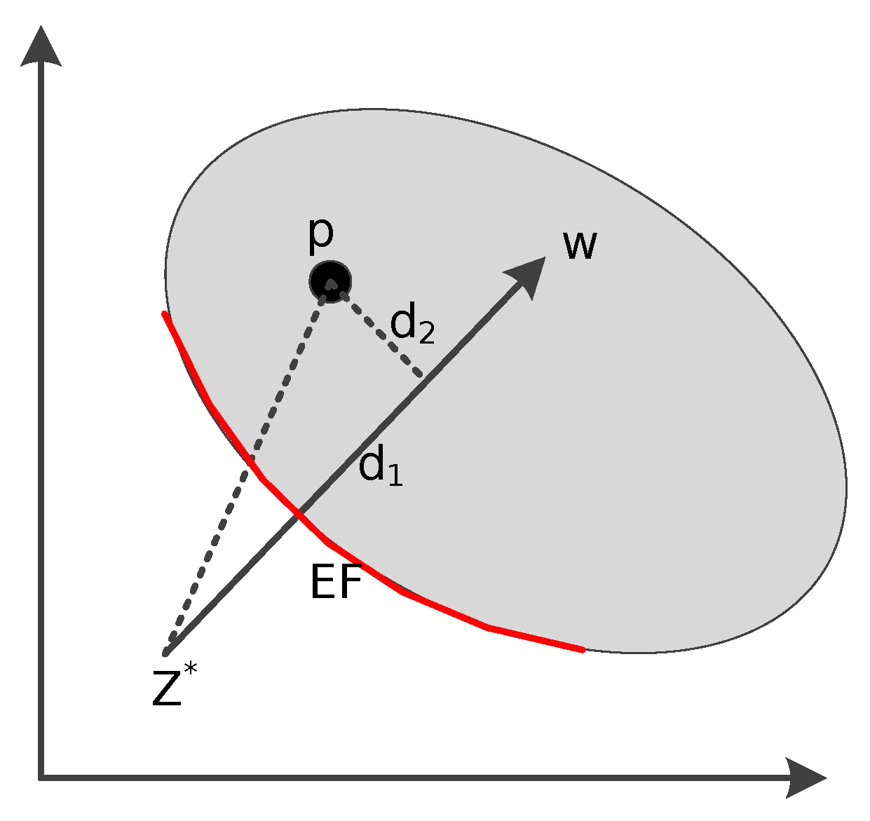
2.2. Penalty Boundary Intersection (PBI) Method

In our work, the penalty boundary intersection (PBI) [24] method is used as the individuals selection method. The optimization problem of the PBI approach is defined as:

$$\left\{\begin{array}{c}min{g}^{p}bi\left(x\right|w,z^{\ast })=d_1+\theta d_2,\hfill \\ subjecttox\in \Omega .\hfill \end{array}\right.$$

(3)

where

$$d_1=\frac{\parallel {(F\left(x\right)-z^{\ast })}^{T}w\parallel }{\parallel w\parallel }$$

(4)

$$d_2=\parallel F\left(x\right)-(z^{\ast }+d_1\frac{w}{\parallel w\parallel })\parallel$$

(5)

$z^{\ast }$ = ${(z_1^{\ast },\dots ,z_m^{\ast })}^T$ is the ideal point of objective space. Normally, we define $\theta \ge 0$ as the penalty parameter. Figure 1 gives a simple schematic illustrating $d_1$ and $d_2$ of a solution x with respect to the weight vector w. In the PBI approach, $d_1$ is used to evaluate the convergence from x to $EF$, and $d_2$ to evaluate the population diversity. By adding the value of $d_2$ multiplied by $\theta$ to $d_1$, $g^{pbi}\left(x\right|w,z^{\ast })$ plays as a composite measure of x for both convergence and diversity.

2.3. Motivation

In the research field of many-objective evolutionary optimization algorithm, as summarized above, they can basically be classified into the above three types. The three types of algorithms have their advantages, but they basically have no intersection. Indicator-based algorithms have good convergence, but they can only rely on other ways to maintain diversity. For example, in PREA, the parallel distance is adopted to improve the population diversity, which makes PREA excellent in solving the problem of irregular PFs. However, because the parallel distance has been used to screen the population throughout the evolutionary process, the final solution may not necessarily be the solution that makes the entire population have the best diversity. This also makes the diversity performance of PREA not as good as that of decomposition-based algorithms when facing regular PFs. Therefore, this paper proposes IDEA to merge indicator-based and decomposition-based algorithms.

As the performance of decomposition-based algorithms sharply drops when solving problems with irregular PFs, an effective reference point adjustment mechanism is needed to ensure the population diversity. The representative method is to adjust the reference point according to the distribution of candidate solutions in each generation of the current population, such as A-NSGA-III and RVEA* [27]. The two groups of reference vectors of RVEA* are adjusted to maintain uniform distribution and to adapt themselves. Reference-vector adaptation involves two operations: (1) deleting each reference vector in the specified empty subspace, and (2) randomly adding new reference vectors to the hyperbox specified by the lowest and ideal point of the current population. Figure 2a presents an example to illustrate this mechanism. The random reference points generated by this method have great randomness and cannot keep uniform distribution on the PFs of MaOPs. This paper improves this method by making the individuals with good distribution become new reference points, which are called anchor points, and its schematic diagram is shown in Figure 2b. The details are introduced in Section 3.

In general, the reference point is also called a reference vector or weight vector in some decomposition-based MOEAs, and in this article, we only use the term reference points.

3. Proposed Algorithm

3.1. Framework

The framework of the IDEA is shown in Algorithm 1. IDEA starts by generating a set of uniformly distributed reference points (To promote diversity in the obtained solutions, Das and Dennis’s systematic approach [42] is adopted to generate structured reference points.); in the meantime, an initial population $P_0$ with size N from the uniform distribution is randomly generated in the objective space. Then, calculate $I_{\infty }^r\left(p_x\right|p_y)$ between any two solutions in $P_t$ by using Equation (2) and save the result in matrix $I_M$; Simultaneously, the individual closest to x is also determined by the indicator $I_{\infty }^r$. The simulated binary crossover and the polynomial mutation are employed on adjacent neighbor solutions to generate an offspring set $Q_t$. After merging $P_t$ and $Q_t$, the environmental selection is implemented. Only when the algorithm determines that the problem is irregular will the reference point adjust by learning population, and the details will be described in the latter.

Algorithm 1 The framework of IDEA.

Input: Population size N, objectives M, the termination criterion; Output: Final population;    1: Generate uniformly distributed reference points $RP$ and an initial population $P_0$;    2: while the termination criterion is not satisfied do    3:     Calculate $I_{\infty }^r\left(p_x\right|p_y)$ between any two solutions by Equation(2) and save the result to matrix $I_M$;    4:     Find neighbor solutions into $S_n$ by using $I_M$;    5:     Crossover and mutation to generate offspring $Q_t$ by using $S_n$;    6:     $P_{(t+1)}$ = EnvironmentalSelection($P_t\bigcup Q_t$, $I_M$, $RP$);    7:     if the problem is irregular then    8:         $RP$ = LearningPopulation($P_{(t+1)}$, N);    9:     end if  10:     t = t+1;  11: end while  12: Return $P_t$;

3.2. Learning Population

After the population has evolved to a certain extent, the individuals obtained through environmental selection have good convergence and distribution. Still, after crossover and mutation, these individuals may be eliminated and selected by the next generation. This problem is even more severe when dealing with irregular PFs. However, we can make the next population better by letting the reference points learn from these individuals. Therefore, we propose a reference point adaptive adjustment method based on the learning population.

The whole process of reference point learning population is given by Algorithm 2. First, the objective values of the selected individuals in the population are taken as a part of the new reference-point set; these are called anchor points. If the number of anchor points multiplied by two is not larger than N, neighbor points are found, and include the generated midpoints into the anchor points. When the condition is not satisfied, the interference reference point is generated. The difference between the maximum value and the minimum value in each dimension is set as the interference factor $\overrightarrow{\delta }$, and then a random number in $[0,{\delta }_i]$ is generated. Then, a point is randomly selected in the anchor set, and the two are added to create an interference-reference point. The interference factor $\overrightarrow{\delta }$ is determined by the following formula:

$$\overrightarrow{\delta }=((f_1^{max}-f_1^{min}),\dots ,(f_m^{max}-f_m^{min})).$$

(6)

When the number of anchor points is greater than N, the Minkowski distance between anchor points is calculated. In order to keep the boundary points better, the Minkowski parameter p is $\frac{1}{m}$, where the m is objectives. The closest points are deleted in sequence until the number of anchor points reaches N.

Algorithm 2 Learning Population.

Input: Population $P_t$, population size N, objectives M; Output: The new reference points $RP$;    1: The objective value of individual in $P_t$ is taken as anchor points $AP$;    2: if the size of $AP$ is smaller than N then    3:     while the size of $AP$ multiplied by 2 is smaller than N do    4:         Calculate the Euclidean distance between $A{P}_i$ and $A{P}_j$;    5:         Find the closest points and calculate their midpoint $M_p$;    6:         $AP$ = $AP\bigcup M_p$;    7:     end while    8:     if the size of $AP$ is smaller than N then    9:         Calculate the interference factor $\overrightarrow{\delta }\in R^M$;  10:         Randomly generate the interference reference point $\overrightarrow{R}\in {[0,\delta ]}^M$;  11:         Randomly select a reference point $P_s\in AP$;  12:         $P_{ir}$ = $P_s+\overrightarrow{R}$;  13:         $AP$ = $AP\bigcup P_{ir}$;  14:     end if  15: else  16:     Delete the nearest point by calculating their Minkowski distance until the number of $AP$ is N;  17: end if  18: Return $AP$

Figure 3 shows a simple example of this procedure. Assuming that the reference points are $N=6$, the black reference points are valid reference points, the gray reference points are invalid reference points, and the red points are individuals bound to the valid reference points, as shown in Figure 3a. First, the objective values of individuals, i.e., red points, are taken as anchor points. Then, the neighbor point is found for every point in anchors, and the midpoints are generated, as shown by the green dots in Figure 3b.

In this case, there are five anchors. Then, the interference-reference points are generated to fill the anchor points. As shown in Figure 3c, the blue point is the interference-reference point.

3.3. Environmental Selection

To maintain population convergence, many decomposition-based algorithms use the traditional Pareto-dominance relationship to exert selection pressure. However, with an increase of objectives, the Pareto-dominance relationship gradually loses selection pressure. This paper uses the $I_{\infty }^r$ indicator introduced above to put selection pressure on the population. When the number of individuals is not larger than N, the population can reproduce through neighbor mating. When the number of individuals exceeds N, environmental selection based on reference points begins.

Algorithm 3 introduces the environmental selection process used in this paper. First, $I_{\infty }^r$ indicator value of individuals is calculated, and individuals whose indicator value is greater than 0 are selected as the nondominant level. If the number of individuals selected in the nondominant level is smaller than N, the population will continue to evolve based on this indicator values. When the number of individuals in the first level is greater than N, the individuals with poor $I_{\infty }^r$ indicator values are deleted, and then bound with the reference points by using the cosine distance. For each effectively bound reference point, the PBI method mentioned above is used to select the individuals with the minimum PBI value of each reference point. It is worth noting that the value of $\theta$ is generally 5, but this paper adopts the following formula to assign value to $\theta$:

$$\theta =k\times \lceil M\times t\rceil$$

(7)

where t is the ratio of the current generation to the maximum generation; M represents the objectives; k is a coefficient and in order to maintain better performance in low-dimensional space, the value of k is 5.

If the proportion of effective reference points is less than 0.8, the problem is considered to be an irregular problem, and a solution to the irregular problems will be implemented. The detail of this part will be introduced in the latter. If the number of selected individuals is greater than N, the operation of deleting individuals introduced in Algorithm 2 is performed until the number of individuals is N.

Algorithm 3 Environmental selection.

Input: Population $P_t$, reference points $RP$, current generation ratio t; Output: The next population $P_{t+1}$;    1: Calculate the matrix of $I_{\infty }^r\left(p_x\right|p_y)$ where $p_x$ and $p_y$ belong to $P_t$, save the result in $I_M$;    2: Find the individuals in the first level by using $I_M$, and save them to $P_{t+1}$;    3: if the size of $P_{t+1}$ is larger than N then    4:     Eliminate the worst individuals by using $I_M$ and create the promising region;    5:     Associate individuals of $P_{t+1}$ with the reference points $RP$ by cosine distance;    6:     for each effective $R{P}_i$ of $RP$ do    7:         Select individuals into $P_{t+1}$ by PBI method and ignore other individuals associated with the same reference point;    8:     end for    9:     if the proportion of effective reference points is smaller than 0.8 then  10:         Implement the procedure of irregular problems and select individuals which aren’t in $P_{t+1}$ into $P_{t+1}$;  11:     end if  12:     if the size of $P_{t+1}$ is larger than N then  13:         Truncate the individuals in $P_{t+1}$ until the number of $P_{t+1}$ is N;  14:     end if  15: end if  16: Return $P_{t+1}$;

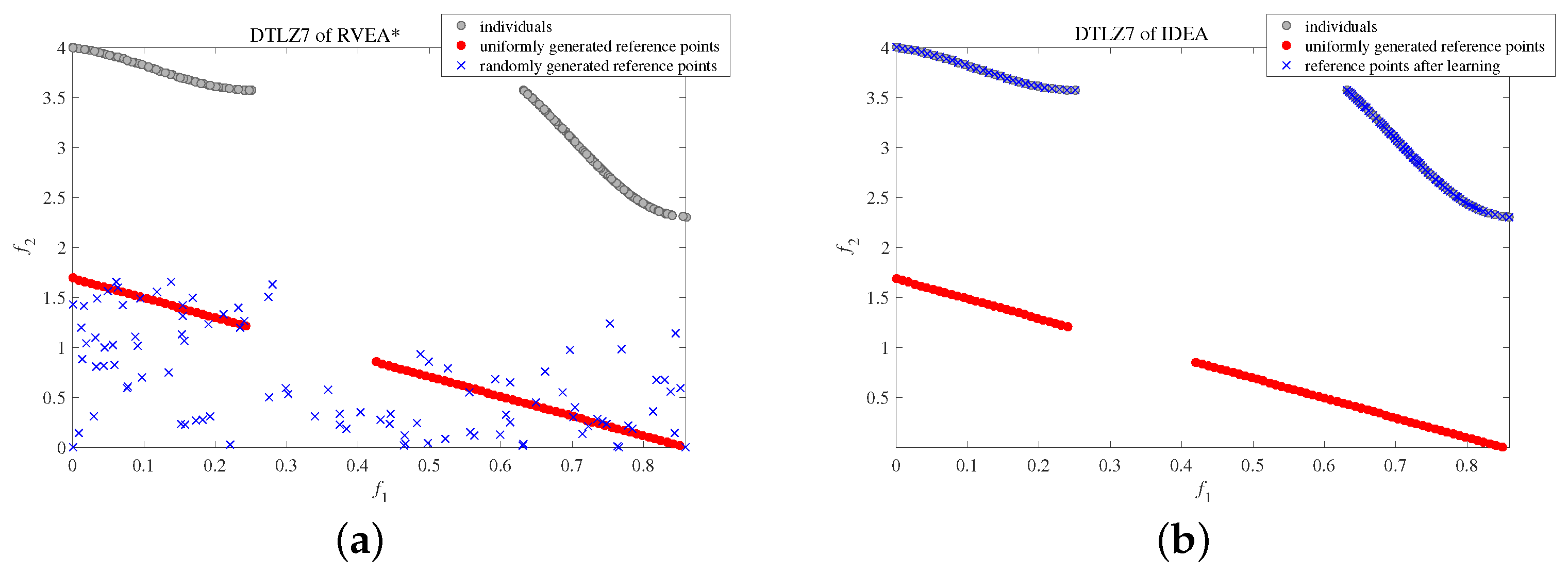
3.4. Handling Irregular Problem

The populations are bound to the reference point by Minkowski distance (This distance has the advantage of keeping the boundary solution of the population, which has been proved in [19]). For each effective binding reference point, the extension distance of the individuals bound on this point is calculated. The individual with the smallest extension distance is taken as the candidate solution. The nearest neighbor of this candidate solution is compared with itself by the $I_{\infty }^r$ indicator, and the individual with a smaller value is selected for the next evolution. The extension distance is determined by the following formula:

$$D_e=\frac{d_2}{d_{\overrightarrow{n}}}$$

(8)

where $d_2$ is the vertical distance of the individual to the vector of the binding reference point; $\overrightarrow{n}$ is the normal vector of the hyperplane specified by ${\sum }_{i=1}^m{f}_i=1$, and $d_n$ is the vertical distance of the individual to $\overrightarrow{n}$.

Figure 4 is an illustration of the extension distance. The red points represent individuals, and the black point is the reference point. The $d_2$ and $d_n$ distance of individual 3 are shown in Figure 4 above. The experiment shows that the population can expand the search boundary on the sharp-tail PFs through the selection of the extended distance.

3.5. Computational Complexity of One Generation of IDEA

The computational complexity of the proposed IDEA approach is mainly contained in lines 3, 6, and 8 of Algorithm 1. Specifically, consider an MaOP with m objectives. Let N be the population size. The computational complexity of constructing the matrix $I_M$ is obviously O($m{N}^2$) in line 3 of Algorithm 1. The strategy of LearningPopulation mainly consists of calculating the midpoint, generating the interference reference point and deleting the nearest point. Calculating the midpoint in line 8 of Algorithm 2 requires O(mN) computations, the computational complexity of generating the interference is O(MN), and then Line 16 in the worst case requires O($N^2$). In environmental selection, the operation of associating a maximum of 2N population members to $H=\left|RP\right|$ reference points would require O($mNH$) computations in line 5 of Algorithm 3. Assuming that L represents the number of individuals associated with a reference point, there are H reference points in the worst cases, thereby requiring larger of O($LH$) computations. Then, the procedure of handling irregular PFs in line 10 of Algorithm 4 mainly consists of operations of associating individuals to reference points and select individuals from promising region. The computational complexity of associating individuals to reference points is O(mNH), the worst case requires O(LH) computations in selecting individuals from promising region formed by H reference points. In practice, the L is far less than M*N, so the computational complexity of environmental selection is O(mNH). Taking into account all the above considerations and calculations, the overall worst-case computational complexity of a generation IDEA is limited by O($m{N}^2$).

Algorithm 4 The procedure of handling irregular PFs.

Input: Population $P_t$, reference points $RP$, objectives M, current generation ratio t; Output: The chosen population $P_c$;    1: Associate individuals of $P_t$ with the reference points $RP$ by Minkowski distance;    2: for each effective $R{P}_i$ of $RP$ do    3:     Select individuals into $P_c$ by the extension distance and ignore other individuals associated with the same reference point;    4: end for    5: Return $P_c$;

4. Experimental Design and Analysis

To study the performance of the proposed IDEA approach, we carried out a series of simulation experiments and compared it with seven EMO algorithms: GrEA, MOEA/DD, MOMBI-II, NSGA-III, RVEA, onebyoneEA [43], VaEA [44], PICEAg [45], KnEA [46] and ENSMOEAD [47]. Among the algorithms compared, MOEA/DD, NSGA-III, RVEA and ENSMOEAD are popular decomposition-based MOEAs, which all showed competitive performance on MOPs and MaOPs with regular PFs; onebyoneEA uses a one-by-one selection strategy that uses three archives to temporarily store individuals. MOMBI-II is an indicator-based MOEA, in which a uniformly distributed set of reference points are used to calculate the $R2$ indicator.

4.1. Experimental Settings

In the experiments, we selected 17 test problems, namely DTLZ1–DTLZ4 [48], IDTLZ1, IDTLZ2 [35], MaF6, MaF7 [49] and WFG1–WFG9 [50] problems, where the specific settings are shown in

Table 1. Settings of the number of objectives, variables and maximum generation for each test problems.

Problem	Number of Objectives (M)	Number of Variables (D)	Number of Generations (${\mathit{G}}_{\mathbf{max}}$)	Pareto Front
Regular Pareto front
DTLZ1	5, 8, 10, 15	M-1 + 5	500	Linear
DTLZ2, 3, 4	5, 8, 10, 15	M-1 + 10	500	Concave
WFG4–9	5, 8, 10, 15	M-1 + 10	1000	Concave
Irregular Pareto front
IDTLZ1	5, 8, 10, 15	M-1 + 5	500	Inverted, Linear
IDTLZ2	5, 8, 10, 15	M-1 + 10	500	Inverted, Concave
MaF6	5, 8, 10, 15	M-1 + 10	500	Degenerate
MaF7	5, 8, 10, 15	M-1 + 20	500	Disconnected
WFG1	5, 8, 10, 15	M-1 + 10	1000	Sharp tails
WFG2	5, 8, 10, 15	M-1 + 10	1000	Disconnected, Sharp tails
WFG3	5, 8, 10, 15	M-1 + 10	1000	Mostly degenerate

The Pareto fronts of WFG3 is also not completely degenerate.

. DTLZ1–DTLZ4 and WFG1– WFG9 are used to test the performance of MOEAs on MOPs and MaOPs since their objective number is flexible. IDTLZ1 and IDTLZ2 represent the problems of inverted DTLZ1 and DTLZ2, respectively, where the regular PFs of DTLZ1 and DTLZ2 are inverted and therefore become irregular [32]. Table 1 indicates the maximum number of generations used for each test problem, and the number of function evaluations for each test problem is population sizes N multiplied by maximum number of generations. As a conclusion, the test problems with irregular PFs include IDTLZ1, IDTLZ2, MaF6, MaF7 and WFG1–WFG3, and the others are with regular PFs.

(1) Reference Points: All algorithms employ the same uniformly distributed reference points with two layers generated by Das and Dennis methods. The

Table 2. The settings of each objective number and relative reference points number, where $p_1$ and $p_2$ denote the number of divisions on each objective in the boundary layer and inner layer.

Number of Objectives (M)	Parameter (${\mathit{p}}_1$, ${\mathit{p}}_2$)	Number of Reference Points
5	5, 0	126
8	3, 2	156
10	2, 2	110
15	2, 1	135

lists the number of reference points for each objectives number, where $p_1$ and $p_2$ represent the numbers of divisions on each objective in the boundary layer and the inner layer, respectively, and the population size of the MOEA for each comparison is the same as the number of reference points.

(2) Parameters in the Compared MOEAs: For MOEA/DD, the size of the neighborhood T is set to $0.1\times N$ where N is the population size, and the neighborhood selection probability $\delta$ was set to 0.9. For RVEA and RVEA*, the penalty parameter $\alpha$ was set to 2, and the reference point adaptive frequency $f_r$ was set to 0.1. For MOMBI-II, the recorded sizes of the variance threshold $\alpha$, tolerance threshold, and nadir vectors were set to 0.5, 0.001, and 5, respectively. However, no additional parameters need to be specified NSGA-III, A-NSGA-III, GrEA, onebyoneEA, and IDEA.

(3) Genetic Operators: The simulated binary crossover (SBX) [51] and polynomial mutation [52] are applied to all MOEAs. The crossover and mutation probabilities were 1.0 and $1/D$ where D is the number of decision variables, and the distribution indexes of both SBX and polynomial mutation were 20.

(4) Performance Metrics: To compare the performance of the algorithms, we considered two widely used quality indicators, such as the inverted generational distance (IGD) [33] and the Hypervolume (HV) [16]. They can evaluate the combined performance of population convergence and diversification. IGD measures the average Euclidean distance from a point evenly distributed along the entire Pareto front to its closet, and smaller values are preferred. The HV is used as an evaluation method to compare the quality of different algorithms. The HV can provide information about both the convergence and distribution of an algorithm, and has been used as a common measure of algorithm performance. It can be expressed as Equation (9), where $S\left(X_i\right)$ is the hypercube qualified by the solution $X_i$ and the reference point r in PF provided by the algorithm. The higher the HV value, the better the result.

$$HV={\cup }_{X_i\in P{F}^{\ast }}S\left(X_i\right).$$

(9)

Before HV calculation, all target values are normalized by the ideal point and the lowest point of the Pareto optimal frontier, and then the reference point r$(1.25,1.25,\dots ,1.25)$ calculates the normalized HV value of the solution set. All the tests were run 20 times independently, and the mean and standard deviation of the IGD and HV metric values were recorded, respectively. The best performing algorithm is highlighted in dark color. The results of the experiment were statistically analyzed using Friedman’s test [53], where the symbols “+”, “−” and ”=” indicate that the results produced by another MOEA are significantly better, significantly worse, or statistically similar to those produced by IDEA.

4.2. Comparisons between IDEA and Existing MOEAs

The statistical results of the IGD and HV values obtained by the ten algorithms over 20 independent runs on regular Pareto front problems are summarized in

Table 3. The statistics of IGD results (mean and standard deviation) on regular Pareto front problems.

Problem	M	NSGA-III	RVEA	MOEA/DD	GrEA	VaEA	onebyoneEA	MOMBI-II	PICEAg	KnEA	ENSMOEAD	IDEA
DTLZ1	5	6.3579e-2 (3.85e-4) =	6.3294e-2 (1.15e-4) =	6.3401e-2 (8.52e-5) =	1.6229e-1 (9.18e-2) -	1.2004e-1 (3.17e-2) -	6.8153e-2 (1.64e-3) -	6.3953e-2 (6.33e-4) =	1.2236e-1 (1.59e-2) -	1.7083e-1 (6.03e-2) -	3.1108e-1 (1.90e-1) -	6.3303e-2 (5.15e-4)
	8	1.2970e-1 (3.44e-2) =	9.7347e-2 (1.06e-3) =	9.5979e-2 (4.47e-4) =	3.3146e-1 (7.39e-2) -	2.7398e-1 (1.60e-1) -	1.1343e-1 (1.35e-3) =	2.1015e-1 (5.20e-2) -	2.3577e-1 (2.64e-2) -	1.3277e+0 (1.39e+0) -	1.7338e-1 (7.83e-2) =	1.0871e-1 (1.21e-2)
	10	2.3492e-1 (1.64e-1) =	1.2014e-1 (1.47e-2) =	1.1358e-1 (7.29e-4) =	1.2515e+0 (3.79e+0) -	4.1036e-1 (1.95e-1) -	1.2826e-1 (1.45e-3) =	2.7082e-1 (1.55e-2) =	3.1488e-1 (1.99e-2) -	8.2622e+0 (5.80e+0) -	3.0006e-1 (3.21e-1) =	1.4973e-1 (2.56e-2)
	15	2.3085e-1 (8.85e-2) =	1.5755e-1 (7.94e-3) +	1.4322e-1 (6.16e-3) =	8.6720e+0 (1.35e+1) -	3.7561e-1 (1.46e-1) -	1.4197e-1 (9.94e-4) =	2.9004e-1 (4.07e-2) =	3.4474e-1 (2.27e-2) -	1.1018e+1 (1.18e+1) -	3.4853e-1 (2.17e-1) -	1.6428e-1 (2.86e-2)
DTLZ2	5	1.9490e-1 (1.90e-5) =	1.9489e-1 (1.30e-5) =	1.9489e-1 (4.15e-6) =	1.9783e-1 (1.14e-3) -	1.9372e-1 (1.21e-3) =	1.9012e-1 (1.66e-3) =	1.9612e-1 (7.66e-4) -	1.9555e-1 (1.28e-3) =	2.1219e-1 (4.55e-3) -	3.2430e-1 (1.63e-3) -	1.9488e-1 (9.50e-6)
	8	3.1627e-1 (7.14e-4) =	3.1545e-1 (1.06e-4) =	3.1507e-1 (4.20e-5) =	3.5079e-1 (1.19e-3) =	3.6360e-1 (2.22e-3) -	3.5058e-1 (2.68e-3) =	3.3129e-1 (1.65e-2) =	3.6333e-1 (1.81e-2) -	3.8349e-1 (6.64e-3) -	5.8962e-1 (1.01e-2) -	3.1652e-1 (3.99e-4)
	10	4.8207e-1 (5.61e-2) -	4.3697e-1 (3.08e-4) =	4.4032e-1 (1.85e-3) =	5.0437e-1 (4.30e-2) -	4.8172e-1 (2.29e-3) -	4.5902e-1 (2.55e-3) -	6.8130e-1 (1.29e-1) -	6.0955e-1 (7.07e-2) -	5.1013e-1 (1.11e-2) -	7.0965e-1 (3.70e-2) -	4.3528e-1 (1.12e-3)
	15	6.4932e-1 (1.56e-2) =	6.2480e-1 (1.76e-3) =	6.2372e-1 (1.36e-3) =	5.9445e-1 (3.01e-2) =	6.0788e-1 (1.43e-2) =	5.5700e-1 (2.97e-3) +	8.5524e-1 (7.99e-2) -	8.3260e-1 (6.06e-2) =	6.1970e-1 (2.23e-2) =	8.8875e-1 (5.53e-2) -	6.2637e-1 (2.11e-3)
DTLZ3	5	1.9490e-1 (1.90e-5) =	1.9489e-1 (1.30e-5) =	1.9489e-1 (4.15e-6) =	1.9783e-1 (1.14e-3) -	1.9372e-1 (1.21e-3) =	1.9012e-1 (1.66e-3) =	1.9612e-1 (7.66e-4) -	1.9555e-1 (1.28e-3) =	2.1219e-1 (4.55e-3) -	3.2430e-1 (1.63e-3) -	1.9488e-1 (9.50e-6)
	8	1.9608e+0 (1.94e+0) =	3.3151e-1 (1.10e-2) +	3.2659e-1 (1.99e-2) +	4.0806e+0 (2.26e+0) =	8.6398e+0 (4.63e+0) =	3.5423e-1 (3.45e-3) +	4.2977e-1 (1.19e-1) +	8.1213e-1 (4.77e-2) =	9.3434e+1 (2.44e+1) -	2.2638e+0 (3.15e+0) =	2.8971e+0 (2.57e+0)
	10	4.6146e+0 (3.53e+0) =	6.8382e-1 (4.15e-1) +	5.6509e-1 (2.48e-1) +	9.2386e+0 (7.11e+0) =	1.8796e+1 (1.39e+1) =	4.6564e-1 (5.15e-3) +	9.9538e-1 (3.58e-2) +	1.0152e+0 (6.17e-2) =	3.3320e+2 (6.58e+1) =	8.1495e+0 (2.37e+1) =	5.8166e+0 (3.01e+0)
	15	6.0731e+0 (3.14e+0) =	8.4420e-1 (3.28e-1) +	6.9215e-1 (2.23e-1) +	1.6914e+2 (6.44e+1) =	1.8080e+1 (7.81e+0) =	5.6388e-1 (5.63e-3) +	1.1035e+0 (9.91e-3) =	1.1634e+0 (3.86e-2) =	5.6540e+2 (1.47e+2) -	1.2181e+1 (3.32e+1) =	7.6826e+0 (1.25e+1)
DTLZ4	5	2.5650e-1 (1.10e-1) =	2.0620e-1 (5.05e-2) +	1.9490e-1 (1.56e-5) +	2.2107e-1 (6.74e-2) =	1.9648e-1 (1.24e-3) =	2.2626e-1 (7.90e-2) +	2.0972e-1 (5.00e-2) =	2.9342e-1 (1.48e-1) =	2.0989e-1 (4.41e-3) +	3.8789e-1 (2.73e-2) =	4.6090e-1 (2.24e-1)
	8	3.6745e-1 (9.41e-2) =	3.2211e-1 (2.49e-2) +	3.2752e-1 (3.64e-2) +	3.5110e-1 (1.30e-3) =	3.6562e-1 (4.41e-3) =	3.6388e-1 (3.11e-2) +	3.6858e-1 (4.53e-2) =	4.2356e-1 (6.31e-2) =	3.7331e-1 (3.71e-3) =	6.5963e-1 (3.73e-2) -	3.9988e-1 (1.11e-1)
	10	4.9913e-1 (7.82e-2) =	4.5270e-1 (2.76e-2) +	4.4793e-1 (2.71e-2) +	4.8914e-1 (1.71e-2) =	4.8594e-1 (3.67e-3) =	4.9508e-1 (5.79e-2) =	5.6311e-1 (6.31e-2) =	6.0235e-1 (5.33e-2) =	5.0342e-1 (7.96e-3) =	8.3599e-1 (5.70e-2) -	5.1001e-1 (5.53e-2)
	15	6.4779e-1 (1.99e-2) =	6.3015e-1 (4.32e-3) =	6.4057e-1 (1.65e-2) =	5.8066e-1 (5.86e-3) +	6.0096e-1 (4.75e-3) +	5.8340e-1 (1.92e-2) +	6.5943e-1 (1.79e-2) =	6.9469e-1 (3.12e-2) =	6.1132e-1 (3.13e-3) =	9.5200e-1 (3.77e-2) -	6.3722e-1 (1.07e-2)
WFG4	5	1.1776e+0 (7.09e-4) =	1.1783e+0 (7.23e-4) =	1.2413e+0 (4.71e-3) =	1.1219e+0 (8.71e-3) =	1.1078e+0 (8.19e-3) +	1.7681e+0 (1.45e-1) -	1.1891e+0 (2.24e-2) =	1.0771e+0 (8.48e-3) +	1.2237e+0 (1.69e-2) =	2.9708e+0 (2.80e-1) -	1.1797e+0 (9.17e-4)
	8	2.9601e+0 (2.83e-3) +	2.9641e+0 (7.53e-3) +	4.1537e+0 (1.44e-1) =	2.8928e+0 (1.18e-2) +	3.0197e+0 (3.82e-2) =	4.3998e+0 (1.78e-1) =	3.3146e+0 (4.04e-1) =	3.4721e+0 (3.76e-1) =	3.3876e+0 (4.15e-2) =	4.6295e+0 (4.73e-1) =	3.6083e+0 (7.19e-2)
	10	5.1162e+0 (5.68e-2) =	4.8764e+0 (3.79e-2) +	6.9056e+0 (2.30e-1) =	5.9090e+0 (3.34e-1) =	4.8985e+0 (3.79e-2) +	6.7965e+0 (2.32e-1) =	8.8996e+0 (1.17e+0) -	7.4339e+0 (5.58e-1) =	5.4820e+0 (5.95e-2) =	7.6371e+0 (5.04e-1) -	6.2367e+0 (2.62e-1)
	15	9.3505e+0 (6.06e-2) =	9.2657e+0 (9.13e-2) =	1.3658e+1 (2.95e-1) =	9.8444e+0 (4.03e-1) =	8.2096e+0 (1.07e-1) +	1.1598e+1 (3.42e-1) =	1.8664e+1 (1.44e+0) -	1.5959e+1 (1.15e+0) -	9.0052e+0 (1.50e-1) +	1.3051e+1 (9.38e-1) =	1.0986e+1 (6.17e-1)
WFG5	5	1.1650e+0 (2.21e-4) =	1.1659e+0 (3.25e-4) =	1.2127e+0 (1.69e-3) =	1.1133e+0 (8.64e-3) =	1.1069e+0 (7.42e-3) =	1.6716e+0 (1.15e-1) -	1.2755e+0 (2.21e-2) -	1.0693e+0 (5.96e-3) +	1.2110e+0 (1.74e-2) =	2.9120e+0 (1.54e-1) -	1.1658e+0 (5.57e-4)
	8	2.9413e+0 (1.83e-3) +	2.9496e+0 (7.27e-3) +	3.9169e+0 (7.34e-2) =	2.8884e+0 (2.00e-2) +	3.0307e+0 (3.74e-2) =	4.2639e+0 (1.90e-1) =	3.5204e+0 (7.06e-2) =	2.9082e+0 (1.73e-2) +	3.3420e+0 (2.50e-2) =	4.8479e+0 (1.27e-1) =	3.6124e+0 (7.47e-2)
	10	5.0775e+0 (7.09e-3) +	4.8100e+0 (2.73e-2) +	6.0792e+0 (1.33e-1) =	6.0173e+0 (6.14e-1) =	4.9262e+0 (4.02e-2) +	6.7113e+0 (1.45e-1) =	1.0592e+1 (4.42e+0) =	6.2535e+0 (2.78e-1) =	5.4942e+0 (5.02e-2) =	7.3569e+0 (2.32e-1) =	6.3355e+0 (8.78e-2)
	15	9.2827e+0 (1.22e-2) =	9.1763e+0 (5.79e-2) +	1.2946e+1 (2.39e-1) =	1.0056e+1 (3.01e-1) =	8.0298e+0 (7.27e-2) +	1.1416e+1 (1.97e-1) =	2.4739e+1 (2.15e+0) -	1.3123e+1 (6.29e-1) =	8.9083e+0 (1.09e-1) +	1.3049e+1 (1.03e+0) =	1.2106e+1 (8.28e-1)
WFG6	5	1.1626e+0 (1.22e-3) =	1.1648e+0 (2.73e-3) +	1.2146e+0 (6.05e-3) =	1.1259e+0 (7.55e-3) =	1.1241e+0 (7.24e-3) =	2.0860e+0 (1.15e-1) -	1.2307e+0 (1.04e-1) =	1.0853e+0 (6.18e-3) +	1.2409e+0 (3.27e-2) =	2.5458e+0 (4.10e-1) -	1.1651e+0 (3.03e-3)
	8	2.9460e+0 (3.14e-3) +	2.9745e+0 (1.33e-2) =	4.0810e+0 (6.91e-2) =	2.9173e+0 (2.24e-2) +	3.1392e+0 (5.51e-2) =	4.9472e+0 (1.21e-1) =	3.0881e+0 (1.91e-1) =	2.9572e+0 (2.51e-2) +	3.4861e+0 (6.04e-2) =	5.5914e+0 (4.23e-1) -	3.4471e+0 (1.34e-1)
	10	5.0931e+0 (8.70e-3) +	5.1861e+0 (1.96e-1) +	6.4001e+0 (3.37e-1) =	5.4470e+0 (3.92e-1) +	4.9780e+0 (5.20e-2) +	7.3785e+0 (1.33e-1) =	6.4436e+0 (1.25e+0) =	5.8329e+0 (3.57e-1) =	5.9158e+0 (3.07e-1) =	8.1136e+0 (4.51e-1) =	6.4897e+0 (2.79e-1)
	15	9.5190e+0 (6.29e-1) +	9.5031e+0 (3.10e-1) =	1.2851e+1 (3.43e-1) =	8.9668e+0 (2.97e-1) +	7.9192e+0 (6.76e-2) +	1.2162e+1 (2.58e-1) =	1.7353e+1 (1.61e+0) -	1.2942e+1 (1.01e+0) =	9.7071e+0 (6.34e-1) =	1.3978e+1 (5.99e-1) =	1.2311e+1 (4.41e-1)
WFG7	5	1.1779e+0 (3.81e-4) =	1.1786e+0 (1.09e-3) =	1.2379e+0 (3.51e-3) =	1.1359e+0 (9.07e-3) =	1.1131e+0 (8.75e-3) +	2.2694e+0 (1.21e-1) -	1.2245e+0 (7.45e-2) =	1.0844e+0 (6.80e-3) +	1.2254e+0 (1.88e-2) =	2.5592e+0 (2.61e-1) -	1.1790e+0 (8.96e-4)
	8	2.9852e+0 (9.46e-2) +	2.9885e+0 (1.73e-2) +	3.6798e+0 (1.36e-1) =	2.9043e+0 (1.41e-2) +	3.0784e+0 (6.18e-2) =	4.7805e+0 (1.97e-1) =	3.0601e+0 (9.20e-2) +	2.9893e+0 (1.36e-1) +	3.3033e+0 (3.71e-2) =	4.8939e+0 (2.67e-1) =	3.6564e+0 (1.02e-1)
	10	5.2801e+0 (2.80e-1) =	4.9728e+0 (8.57e-2) +	6.1055e+0 (1.52e-1) =	5.3889e+0 (3.53e-1) =	4.8913e+0 (4.64e-2) +	7.0929e+0 (2.82e-1) =	7.0331e+0 (1.26e+0) =	5.8424e+0 (6.40e-1) =	5.3193e+0 (1.14e-1) =	7.8188e+0 (1.82e-1) -	6.1075e+0 (2.30e-1)
	15	9.2938e+0 (1.68e-1) =	9.3590e+0 (8.87e-2) =	1.3230e+1 (3.87e-1) =	9.2634e+0 (4.00e-1) =	8.0336e+0 (6.99e-2) +	1.1447e+1 (5.49e-1) =	1.6107e+1 (2.10e+0) -	1.2709e+1 (1.49e+0) =	8.6518e+0 (2.79e-1) +	1.4471e+1 (1.06e+0) -	1.0748e+1 (6.52e-1)
WFG8	5	1.1472e+0 (1.02e-3) =	1.1661e+0 (1.10e-3) =	1.2162e+0 (5.84e-3) =	1.1400e+0 (1.09e-2) =	1.2054e+0 (1.74e-2) =	1.8335e+0 (8.53e-2) -	2.9663e+0 (2.33e-2) -	1.1592e+0 (9.69e-3) =	1.2972e+0 (1.82e-2) -	3.3784e+0 (1.37e-1) -	1.1650e+0 (7.49e-3)
	8	3.3276e+0 (2.49e-1) =	3.0507e+0 (2.76e-2) =	3.7669e+0 (2.90e-1) -	3.0518e+0 (5.11e-2) =	3.2510e+0 (3.13e-2) =	4.5738e+0 (2.91e-1) -	3.9781e+0 (2.19e-1) -	3.6896e+0 (1.75e-1) -	3.5565e+0 (5.96e-2) =	5.5816e+0 (1.52e-1) -	3.1320e+0 (4.87e-2)
	10	5.2787e+0 (2.05e-1) =	5.4241e+0 (1.50e-1) =	6.2102e+0 (3.92e-1) =	6.1006e+0 (5.27e-2) =	5.1295e+0 (3.59e-2) =	6.9828e+0 (3.19e-1) -	9.8525e+0 (8.61e-1) -	6.5333e+0 (3.65e-1) -	5.6690e+0 (3.30e-1) =	7.7547e+0 (3.17e-1) -	5.4545e+0 (1.98e-1)
	15	9.2269e+0 (3.50e-1) =	9.3722e+0 (4.12e-1) =	1.0130e+1 (1.41e+0) =	1.0471e+1 (9.74e-2) =	8.5626e+0 (1.43e-1) =	1.1563e+1 (6.16e-1) =	2.0496e+1 (1.31e+0) -	1.3563e+1 (7.97e-1) -	9.9974e+0 (6.57e-1) =	1.6032e+1 (1.23e+0) -	9.6539e+0 (4.88e-1)
WFG9	5	1.1341e+0 (4.81e-3) =	1.1516e+0 (2.23e-3) =	1.2059e+0 (7.03e-3) =	1.0822e+0 (7.74e-3) +	1.0869e+0 (1.39e-2) =	1.6886e+0 (1.23e-1) =	2.3146e+0 (2.54e-1) -	1.0572e+0 (8.93e-3) +	1.1729e+0 (1.62e-2) =	2.9145e+0 (1.98e-1) -	1.1538e+0 (2.79e-3)
	8	2.9247e+0 (7.03e-3) +	2.9414e+0 (1.35e-2) +	3.9840e+0 (1.80e-1) =	2.9086e+0 (1.09e-2) +	3.0113e+0 (3.37e-2) =	4.2097e+0 (1.56e-1) =	3.7008e+0 (2.65e-2) =	2.9851e+0 (1.68e-1) +	3.2511e+0 (1.97e-2) =	5.1840e+0 (3.02e-1) -	3.7019e+0 (1.40e-1)
	10	5.0369e+0 (6.00e-2) +	4.8586e+0 (4.37e-2) +	5.8592e+0 (1.71e-1) =	5.8720e+0 (3.64e-1) =	4.8288e+0 (4.52e-2) +	6.2180e+0 (2.16e-1) =	9.4215e+0 (4.85e+0) -	6.0315e+0 (4.38e-1) =	5.2228e+0 (6.75e-2) +	7.3969e+0 (5.36e-1) -	6.1223e+0 (2.84e-1)
	15	8.8033e+0 (1.31e-1) +	9.1527e+0 (1.13e-1) =	1.1313e+1 (2.56e-1) =	9.4323e+0 (3.35e-1) =	7.7558e+0 (6.43e-2) +	1.0228e+1 (3.92e-1) =	2.5788e+1 (2.36e+0) -	1.3614e+1 (5.47e-1) =	8.2391e+0 (1.93e-1) +	1.3847e+1 (1.03e+0) =	1.1519e+1 (1.06e+0)
+/−/=		10/1/29	18/0/22	6/1/33	9/7/24	13/7/20	6/9/23	3/17/20	9/10/21	6/10/24	0/25/15

Values with a gray background and bold indicate the highest performing values.

and

Table 4. The statistics of HV results (mean and standard deviation) on regular Pareto front problems.

Problem	M	NSGA-III	RVEA	MOEA/DD	GrEA	VaEA	onebyoneEA	MOMBI-II	PICEAg	KnEA	ENSMOEAD	IDEA
DTLZ1	5	9.7445e-1 (6.83e-4) =	9.7474e-1 (1.99e-4) =	9.7480e-1 (1.78e-4) =	7.2922e-1 (1.94e-1) -	8.7340e-1 (5.27e-2) -	9.1956e-1 (6.91e-3) -	9.7386e-1 (1.41e-3) =	9.2996e-1 (2.24e-2) -	6.8276e-1 (1.34e-1) -	4.4217e-1 (3.72e-1) -	9.7449e-1 (1.06e-3)
	8	9.7859e-1 (3.44e-2) =	9.9749e-1 (1.30e-4) =	9.9723e-1 (1.64e-4) =	5.3977e-1 (2.04e-1) -	7.2531e-1 (3.36e-1) -	9.7544e-1 (4.21e-3) =	9.1470e-1 (6.96e-2) -	9.0165e-1 (4.62e-2) -	1.5301e-1 (3.15e-1) -	8.8629e-1 (2.08e-1) -	9.9651e-1 (1.42e-3)
	10	7.9573e-1 (3.40e-1) =	9.9041e-1 (9.60e-3) -	9.5904e-1 (1.28e-2) =	3.6111e-1 (2.14e-1) -	4.5272e-1 (3.88e-1) -	9.7933e-1 (4.65e-3) =	8.1983e-1 (5.88e-2) -	7.7192e-1 (8.24e-2) -	0.0000e+0 (0.00e+0) -	7.2894e-1 (3.40e-1) -	9.9135e-1 (5.89e-3)
	15	8.9601e-1 (2.27e-1) =	9.9864e-1 (8.66e-4) =	9.8946e-1 (8.74e-3) =	1.9429e-1 (2.46e-1) -	5.1852e-1 (3.52e-1) -	9.8989e-1 (2.84e-3) =	7.8704e-1 (1.19e-1) -	7.4953e-1 (8.65e-2) -	0.0000e+0 (0.00e+0) -	5.4963e-1 (3.59e-1) -	9.7005e-1 (1.01e-1)
DTLZ2	5	7.9452e-1 (4.77e-4) =	7.9475e-1 (4.11e-4) =	7.9477e-1 (4.59e-4) =	7.9196e-1 (1.10e-3) -	7.7502e-1 (2.98e-3) -	7.7772e-1 (4.05e-3) -	7.9364e-1 (4.30e-4) =	7.7787e-1 (2.61e-3) -	7.7067e-1 (5.90e-3) -	6.9113e-1 (8.31e-3) -	7.9494e-1 (4.32e-4)
	8	9.2286e-1 (5.93e-4) =	9.2373e-1 (2.45e-4) =	9.2381e-1 (1.95e-4) =	9.0219e-1 (1.77e-3) -	9.0306e-1 (3.26e-3) -	9.0561e-1 (3.79e-3) -	9.2462e-1 (4.94e-3) =	9.0145e-1 (1.63e-2) -	8.8595e-1 (8.16e-3) -	5.4370e-1 (1.93e-2) -	9.2430e-1 (3.58e-4)
	10	9.1759e-1 (3.01e-2) -	9.4299e-1 (5.86e-4) =	8.9676e-1 (3.32e-2) -	9.4257e-1 (1.92e-2) =	9.1212e-1 (4.04e-3) -	9.2510e-1 (3.60e-3) =	7.9448e-1 (9.91e-2) -	8.1240e-1 (5.25e-2) -	9.3591e-1 (1.38e-2) =	3.7185e-1 (2.28e-2) -	9.4411e-1 (2.74e-4)
	15	9.7239e-1 (1.07e-2) -	9.9001e-1 (1.66e-3) =	9.9036e-1 (1.01e-4) =	9.7722e-1 (9.02e-3) =	9.0601e-1 (3.17e-2) -	9.6215e-1 (2.51e-3) -	8.1797e-1 (9.12e-2) -	8.1531e-1 (6.11e-2) -	9.7122e-1 (2.44e-2) =	3.3299e-1 (2.04e-2) -	9.8909e-1 (3.21e-3)
DTLZ3	5	6.7969e-1 (2.16e-1) =	6.9463e-1 (2.38e-1) =	7.7565e-1 (9.61e-3) =	2.5930e-1 (1.28e-1) -	4.0105e-1 (2.12e-1) -	7.3334e-1 (1.73e-1) =	7.7908e-1 (6.79e-3) =	5.6362e-1 (3.88e-2) =	5.8856e-1 (1.53e-1) =	8.1682e-2 (1.31e-1) -	7.2889e-1 (1.68e-1)
	8	1.9320e-1 (3.21e-1) =	9.0302e-1 (1.62e-2) +	9.0340e-1 (2.66e-2) +	2.4037e-3 (1.07e-2) =	0.0000e+0 (0.00e+0) =	8.9914e-1 (3.49e-3) +	8.8245e-1 (6.73e-2) +	3.7344e-1 (5.45e-2) =	0.0000e+0 (0.00e+0) =	3.0866e-1 (2.38e-1) =	1.5318e-1 (2.86e-1)
	10	6.1488e-2 (1.89e-1) =	6.6707e-1 (3.95e-1) +	5.9787e-1 (2.85e-1) +	0.0000e+0 (0.00e+0) =	0.0000e+0 (0.00e+0) =	9.0792e-1 (1.71e-2) +	4.0882e-1 (6.39e-2) +	2.4789e-1 (5.09e-2) +	0.0000e+0 (0.00e+0) =	1.6483e-1 (1.71e-1) =	8.3074e-3 (3.72e-2)
	15	2.6072e-2 (1.17e-1) -	7.1219e-1 (4.32e-1) +	8.8444e-1 (3.03e-1) +	0.0000e+0 (0.00e+0) =	0.0000e+0 (0.00e+0) =	9.5603e-1 (7.09e-3) +	4.1409e-1 (1.40e-2) +	2.0381e-1 (5.24e-2) +	0.0000e+0 (0.00e+0) =	1.6375e-1 (1.61e-1) =	3.3290e-2 (1.49e-1)
DTLZ4	5	7.5819e-1 (6.72e-2) +	7.9009e-1 (2.05e-2) +	7.9489e-1 (3.71e-4) +	7.8263e-1 (2.93e-2) =	7.7286e-1 (2.72e-3) =	7.7485e-1 (3.20e-2) =	7.8840e-1 (1.99e-2) =	7.3467e-1 (7.13e-2) =	7.7713e-1 (4.36e-3) =	6.5731e-1 (2.34e-2) =	6.5151e-1 (1.40e-1)
	8	9.0144e-1 (4.70e-2) =	9.2273e-1 (5.05e-3) =	9.2005e-1 (1.23e-2) =	9.0529e-1 (2.44e-3) =	8.9471e-1 (7.63e-3) -	9.1400e-1 (8.62e-3) =	9.2243e-1 (1.35e-2) =	8.8648e-1 (2.37e-2) =	9.0248e-1 (4.71e-3) =	6.2783e-1 (1.50e-2) -	8.9543e-1 (4.67e-2)
	10	9.1619e-1 (3.44e-2) =	9.3739e-1 (1.04e-2) =	9.3990e-1 (8.71e-3) +	9.5028e-1 (6.66e-3) +	9.1340e-1 (5.26e-3) =	9.2854e-1 (2.45e-2) =	9.0488e-1 (4.29e-2) =	8.7536e-1 (2.80e-2) =	9.3980e-1 (7.57e-3) =	5.0318e-1 (1.71e-2) -	9.0367e-1 (3.34e-2)
	15	9.7878e-1 (1.38e-2) =	9.9006e-1 (1.58e-3) =	9.8737e-1 (5.21e-3) =	9.8316e-1 (1.53e-3) =	9.4736e-1 (6.36e-3) -	9.7632e-1 (3.98e-3) -	9.8177e-1 (6.27e-3) =	9.3833e-1 (1.61e-2) -	9.8405e-1 (1.37e-3) =	4.6594e-1 (2.54e-2) -	9.8540e-1 (6.36e-3)
WFG4	5	7.9181e-1 (9.28e-4) =	7.9117e-1 (7.27e-4) =	7.5901e-1 (3.01e-3) -	7.7689e-1 (2.19e-3) -	7.5984e-1 (3.45e-3) -	6.4131e-1 (1.67e-2) -	7.9177e-1 (4.54e-3) =	7.6781e-1 (3.65e-3) -	7.7018e-1 (2.76e-3) -	5.1390e-1 (3.59e-2) -	7.9441e-1 (3.99e-4)
	8	9.1731e-1 (1.18e-3) =	9.1490e-1 (1.57e-3) =	8.0047e-1 (1.82e-2) -	8.6480e-1 (3.28e-3) =	8.8394e-1 (6.74e-3) =	7.4214e-1 (1.48e-2) -	8.8688e-1 (5.35e-2) =	8.2498e-1 (4.13e-2) =	9.0910e-1 (2.06e-3) =	6.5714e-1 (4.93e-2) -	8.9440e-1 (4.02e-3)
	10	9.2661e-1 (1.43e-2) +	9.2341e-1 (6.36e-3) =	7.8139e-1 (2.12e-2) =	8.5246e-1 (1.86e-2) =	8.9702e-1 (5.20e-3) =	7.5910e-1 (1.44e-2) =	6.1392e-1 (6.58e-2) -	7.1772e-1 (4.83e-2) =	9.4481e-1 (2.19e-3) +	5.0636e-1 (5.61e-2) -	8.2188e-1 (3.36e-2)
	15	9.8426e-1 (3.06e-3) +	9.8066e-1 (2.29e-3) =	6.3829e-1 (3.53e-2) -	9.2764e-1 (9.45e-3) =	9.2742e-1 (6.45e-3) =	8.3187e-1 (9.58e-3) =	5.7310e-1 (7.35e-2) -	7.1063e-1 (5.61e-2) =	9.8284e-1 (1.19e-3) +	5.8568e-1 (9.44e-2) -	8.8006e-1 (1.96e-2)
WFG5	5	7.4401e-1 (2.81e-4) =	7.4369e-1 (4.97e-4) =	7.1779e-1 (9.38e-4) -	7.3684e-1 (2.15e-3) =	7.1999e-1 (3.92e-3) -	6.0838e-1 (1.53e-2) -	7.1703e-1 (7.74e-3) -	7.2217e-1 (2.24e-3) -	7.2455e-1 (4.38e-3) -	4.6665e-1 (3.40e-2) -	7.4382e-1 (4.31e-4)
	8	8.6286e-1 (4.22e-4) +	8.6201e-1 (5.63e-4) =	7.7454e-1 (7.56e-3) =	8.2472e-1 (4.21e-3) =	8.3507e-1 (3.56e-3) =	7.0016e-1 (1.95e-2) -	7.7164e-1 (1.48e-2) =	8.3767e-1 (2.27e-3) =	8.4466e-1 (2.75e-3) =	5.8823e-1 (3.12e-2) -	8.3371e-1 (6.76e-3)
	10	8.7483e-1 (1.11e-3) =	8.7858e-1 (7.04e-4) =	7.6553e-1 (1.54e-2) =	7.9456e-1 (5.63e-2) =	8.3937e-1 (3.76e-3) =	7.0823e-1 (1.10e-2) =	4.5913e-1 (2.33e-1) -	6.8096e-1 (1.96e-2) -	8.8309e-1 (1.84e-3) +	5.1575e-1 (3.29e-2) -	7.8965e-1 (4.23e-3)
	15	9.1576e-1 (2.29e-3) +	9.1693e-1 (1.97e-4) +	6.0793e-1 (1.82e-2) =	8.3840e-1 (7.57e-3) =	8.6302e-1 (3.57e-3) =	7.7648e-1 (8.71e-3) =	2.6015e-1 (8.40e-2) -	6.7442e-1 (3.35e-2) =	9.1170e-1 (9.17e-4) =	5.5500e-1 (2.57e-2) -	8.1591e-1 (1.44e-2)
WFG6	5	7.2318e-1 (1.10e-2) =	7.2920e-1 (1.97e-2) =	6.8940e-1 (1.97e-2) -	7.2182e-1 (1.23e-2) =	7.0264e-1 (1.23e-2) -	5.3602e-1 (2.83e-2) -	7.2550e-1 (1.81e-2) =	7.0845e-1 (1.03e-2) =	7.0327e-1 (1.40e-2) -	4.6102e-1 (6.92e-2) -	7.3274e-1 (1.76e-2)
	8	8.3760e-1 (1.30e-2) =	8.3307e-1 (1.55e-2) =	7.2865e-1 (2.67e-2) =	8.1120e-1 (1.75e-2) =	8.2292e-1 (1.23e-2) =	6.0933e-1 (2.77e-2) -	8.3858e-1 (2.35e-2) =	8.2080e-1 (1.38e-2) =	8.1567e-1 (2.53e-2) =	5.1901e-1 (8.42e-2) -	8.1384e-1 (2.19e-2)
	10	8.4862e-1 (2.08e-2) +	7.1195e-1 (7.33e-2) =	6.8971e-1 (7.31e-2) =	8.1882e-1 (3.61e-2) =	8.3499e-1 (1.90e-2) +	6.0902e-1 (3.15e-2) =	6.6231e-1 (8.72e-2) =	7.1181e-1 (3.15e-2) =	8.5282e-1 (2.58e-2) +	3.7456e-1 (7.60e-2) -	7.2360e-1 (3.88e-2)
	15	8.7959e-1 (2.04e-2) +	7.6000e-1 (6.03e-2) =	5.8484e-1 (3.85e-2) =	8.5613e-1 (3.25e-2) +	8.7018e-1 (2.34e-2) +	6.8213e-1 (3.13e-2) =	4.8279e-1 (9.63e-2) -	7.0208e-1 (6.24e-2) =	8.7608e-1 (3.07e-2) +	3.8271e-1 (1.50e-1) -	7.1964e-1 (3.65e-2)
WFG7	5	7.9232e-1 (5.58e-4) =	7.9020e-1 (5.84e-4) =	7.6258e-1 (3.26e-3) -	7.9198e-1 (1.23e-3) =	7.7048e-1 (3.26e-3) -	5.7933e-1 (1.57e-2) -	7.8755e-1 (1.14e-2) =	7.7235e-1 (2.39e-3) -	7.7682e-1 (3.92e-3) -	5.5536e-1 (5.85e-2) -	7.9267e-1 (7.07e-4)
	8	9.1731e-1 (8.91e-3) +	9.0906e-1 (2.65e-3) +	8.5204e-1 (1.46e-2) =	8.8829e-1 (3.16e-3) =	9.0314e-1 (2.47e-3) =	6.9558e-1 (1.44e-2) -	9.1987e-1 (8.57e-3) +	8.8851e-1 (2.54e-2) =	8.9282e-1 (6.59e-3) =	6.5626e-1 (3.85e-2) -	8.8981e-1 (7.83e-3)
	10	9.1643e-1 (2.66e-2) +	9.1581e-1 (1.48e-2) +	8.4180e-1 (1.91e-2) =	9.0144e-1 (3.72e-2) +	9.1959e-1 (2.29e-3) +	7.1700e-1 (1.20e-2) =	7.0793e-1 (9.88e-2) =	7.9733e-1 (5.99e-2) =	9.4092e-1 (6.13e-3) +	4.9267e-1 (4.28e-2) =	7.8561e-1 (5.93e-2)
	15	9.7867e-1 (8.20e-3) +	9.6776e-1 (1.64e-2) =	7.2921e-1 (2.71e-2) -	9.4505e-1 (1.02e-2) =	9.5253e-1 (3.55e-3) =	8.3546e-1 (1.05e-2) =	6.5207e-1 (1.37e-1) -	8.0399e-1 (7.26e-2) =	9.7224e-1 (2.25e-2) +	5.1957e-1 (4.19e-2) -	9.1922e-1 (2.21e-2)
WFG8	5	6.8384e-1 (1.74e-3) =	6.7482e-1 (1.90e-3) =	6.6150e-1 (5.30e-3) =	6.7519e-1 (3.51e-3) =	6.3141e-1 (1.02e-2) -	4.9476e-1 (2.52e-2) -	3.1729e-1 (5.04e-3) -	6.3802e-1 (7.53e-3) -	6.4122e-1 (3.73e-3) -	2.5469e-1 (2.45e-2) -	6.8862e-1 (1.84e-2)
	8	7.8235e-1 (1.58e-2) =	7.5333e-1 (5.05e-2) =	7.0989e-1 (5.57e-2) -	7.4690e-1 (2.93e-2) -	7.1925e-1 (1.32e-2) -	4.9836e-1 (4.64e-2) -	5.9695e-1 (1.62e-2) -	7.5766e-1 (5.69e-3) =	7.6525e-1 (2.14e-2) =	3.3579e-1 (3.54e-2) -	7.9681e-1 (1.82e-2)
	10	7.7140e-1 (2.08e-2) -	6.7892e-1 (1.03e-1) =	5.4606e-1 (9.19e-2) -	8.3029e-1 (3.51e-3) =	7.6167e-1 (1.31e-2) =	4.4671e-1 (1.05e-1) -	5.0403e-1 (5.99e-2) -	7.4356e-1 (3.18e-2) =	8.3607e-1 (1.61e-2) =	3.3122e-1 (6.65e-2) -	7.8217e-1 (4.05e-2)
	15	8.9846e-1 (3.27e-2) =	6.2231e-1 (1.51e-1) =	7.8402e-1 (1.61e-1) =	8.9771e-1 (3.46e-3) =	8.3930e-1 (1.18e-2) =	4.9365e-1 (1.21e-1) =	3.5405e-1 (2.93e-2) -	7.5496e-1 (4.13e-2) =	9.0642e-1 (3.28e-2) =	3.5295e-1 (4.79e-2) -	7.7807e-1 (9.72e-2)
WFG9	5	7.4945e-1 (3.96e-3) =	7.5331e-1 (2.64e-3) =	7.0773e-1 (1.05e-2) -	7.4748e-1 (4.00e-3) =	7.1279e-1 (3.10e-2) -	6.0632e-1 (2.27e-2) -	5.4358e-1 (6.03e-2) -	7.4085e-1 (1.04e-2) =	7.4861e-1 (4.56e-3) =	4.7813e-1 (7.60e-2) -	7.5359e-1 (6.59e-3)
	8	8.5651e-1 (1.02e-2) =	8.4512e-1 (2.11e-2) =	7.3318e-1 (3.11e-2) -	8.1055e-1 (6.25e-3) =	8.0206e-1 (4.38e-2) =	6.9038e-1 (1.70e-2) -	7.3246e-1 (4.16e-2) =	8.3368e-1 (4.61e-2) =	8.6422e-1 (5.93e-3) +	5.0669e-1 (5.87e-2) -	8.2049e-1 (1.04e-2)
	10	8.1980e-1 (4.00e-2) +	8.3437e-1 (4.86e-2) +	6.8055e-1 (4.60e-2) =	8.0898e-1 (2.22e-2) +	7.2545e-1 (7.49e-2) =	6.9802e-1 (3.01e-2) =	5.4897e-1 (2.51e-1) -	7.2526e-1 (3.28e-2) =	8.4307e-1 (7.94e-2) +	4.7902e-1 (7.68e-2) -	7.3618e-1 (4.35e-2)
	15	8.7522e-1 (6.70e-2) =	8.0448e-1 (8.41e-2) =	5.3211e-1 (6.45e-2) =	8.7297e-1 (7.29e-3) =	7.7153e-1 (7.07e-2) =	7.2418e-1 (3.96e-2) =	2.3669e-1 (8.53e-2) -	7.0360e-1 (2.14e-2) =	8.7984e-1 (6.84e-2) +	3.7213e-1 (5.37e-2) -	7.5320e-1 (6.12e-2)
+/−/=		11/4/25	8/1/31	5/12/23	4/9/27	3/18/19	3/18/19	4/19/17	2/14/24	10/11/19	0/35/5

Values with a gray background and bold indicate the highest performing values.

, where the best results are highlighted. As shown in tables with results of IGD and HV, when solving test problems with regular PFs, IDEA achieved the competitive performance on most test problems. Compared with traditional decomposition-based algorithm, such as NSGA-III, RVEA, MOEA/DD and ENSMOEAD, IDEA shows the best performance on the 10-objective DTLZ2 instance and WFG4 to WFG9 instances in term of the different number of objectives, and it also can be seen that RVEA and MOEA/DD are encouraging, especially on DTLZ instances with regular PFs. For modified dominance-based algorithms, such as GrEA and KnEA, from the result data shown in Table 3 and Table 4, IDEA has a better performance, which is most likely because these algorithms all pay more attentions on the modified Pareto-domination relationship to provide selection pressure, but less consideration of diversity. Additionally, when GrEA solves problems of different dimensions, it gives different numbers of grid divisions. Under these specific grid parameters, the performance of GrEA is greatly improved, and the advantage of IDEA is that there is no need to set specific parameters. For onebyoneEA, it is shown that the algorithm is highly competitive on relatively simple DTLZ test problems, but it can be seen that it is not as good as IDEA when solving the WFG instance with regular PFs, mainly because IDEA has a selection part based on decomposition to expand the diversity of the algorithm when dealing with more complicated problems. Compared with the indicator-based algorithm, such as MOMBI-II, it can be seen that IDEA is more competitive. This is mainly because IDEA introduces reference points to guide the diversity of individuals in the population. AS shown in Table 4, the overall performance is generally good. Specifically, the proposed IDEA is better than all compared algorithms on the DTLZ2 with 5-objective and 10-objective. Specially, as can be observed in Table 4, IDEA shows the competitive performance on the WFG5 to WFG9 with different difficulties in the decision space. By contrast, KnEA shows promising performance on some 10-objective instances. RVEA and MOEA/DD also show generally competitive performance on DTLZ1 to DTLZ4.

The statistical IGD and HV results obtained by the eleven compared algorithms on irregular Pareto front problems are summarized in

Table 5. The statistics of IGD results (mean and standard deviation ) on irregular Pareto front problems.

Problem	M	NSGA-III	RVEA	MOEA/DD	GrEA	VaEA	onebyoneEA	MOMBI-II	PICEAg	KnEA	ENSMOEAD	IDEA
WFG1	5	4.3763e-1 (2.48e-3) =	4.2703e-1 (7.27e-3) =	5.7320e-1 (2.76e-2) -	5.2792e-1 (1.65e-2) -	4.3439e-1 (5.09e-3) =	7.7381e-1 (4.11e-2) -	4.8710e-1 (5.33e-2) =	6.3240e-1 (2.74e-1) -	4.7835e-1 (8.50e-3) =	1.3799e+0 (7.74e-2) -	4.3896e-1 (1.35e-2)
	8	8.5684e-1 (1.70e-2) +	9.9409e-1 (2.61e-2) =	1.2687e+0 (3.09e-2) =	1.2958e+0 (1.05e-1) =	8.5863e-1 (1.80e-2) +	1.6551e+0 (5.31e-2) -	1.0137e+0 (4.70e-2) =	1.2428e+0 (1.67e-1) =	9.1226e-1 (2.05e-2) =	1.9021e+0 (9.12e-2) -	1.0714e+0 (6.72e-2)
	10	1.1045e+0 (4.14e-2) +	1.1803e+0 (5.01e-2) =	1.3073e+0 (4.98e-2) =	1.2322e+0 (3.73e-2) =	1.1649e+0 (3.77e-2) =	1.8378e+0 (4.75e-2) -	1.6505e+0 (2.87e-1) =	1.7124e+0 (1.10e-1) =	1.2300e+0 (5.48e-2) =	2.2529e+0 (1.35e-1) -	1.2659e+0 (7.63e-2)
	15	1.7627e+0 (1.73e-1) =	1.7656e+0 (8.18e-2) =	2.0243e+0 (4.21e-2) -	2.1833e+0 (8.03e-2) =	1.6914e+0 (4.07e-2) +	2.4310e+0 (2.93e-2) -	2.3159e+0 (3.44e-1) =	2.3973e+0 (1.71e-1) -	1.7580e+0 (8.89e-2) =	2.4192e+0 (1.12e-1) -	2.0205e+0 (1.38e-1)
WFG2	5	4.7258e-1 (1.61e-3) =	4.4635e-1 (7.97e-3) +	5.9445e-1 (1.75e-2) -	5.1884e-1 (1.93e-2) =	4.5852e-1 (1.06e-2) =	7.5509e-1 (6.80e-2) -	4.9571e-1 (5.82e-2) =	5.1193e-1 (1.41e-2) =	5.3244e-1 (2.11e-2) =	1.2339e+0 (1.61e-1) -	4.9566e-1 (1.20e-2)
	8	1.0251e+0 (1.49e-1) +	9.8987e-1 (3.76e-2) +	1.3887e+0 (7.41e-3) =	9.9952e-1 (4.00e-2) +	9.3494e-1 (1.36e-2) +	1.7585e+0 (5.83e-2) =	1.1633e+0 (8.18e-2) =	1.1219e+0 (6.75e-2) =	1.0754e+0 (2.65e-2) =	1.6155e+0 (1.45e-1) =	1.2565e+0 (7.91e-2)
	10	1.2731e+0 (1.10e-1) +	1.3391e+0 (5.43e-2) =	1.3921e+0 (2.79e-2) =	1.2425e+0 (3.07e-2) +	1.2704e+0 (2.75e-2) +	1.9548e+0 (3.12e-2) =	3.6023e+0 (1.31e+0) -	1.7745e+0 (1.24e-1) =	1.3538e+0 (5.68e-2) =	1.9002e+0 (1.18e-1) =	1.4900e+0 (7.45e-2)
	15	1.7568e+0 (7.68e-2) +	1.8593e+0 (7.82e-2) =	2.1867e+0 (1.28e-2) =	1.9310e+0 (7.96e-2) =	1.7408e+0 (4.06e-2) +	2.5204e+0 (3.41e-2) =	6.6940e+0 (2.93e+0) -	3.4687e+0 (8.07e-1) -	2.1834e+0 (6.70e-1) =	2.4038e+0 (1.86e-1) =	2.0867e+0 (6.94e-2)
WFG3	5	5.7985e-1 (5.75e-2) =	5.3607e-1 (2.44e-2) =	6.5151e-1 (1.60e-2) -	3.9129e-1 (5.46e-2) =	6.4405e-1 (5.43e-2) -	1.3522e+0 (1.38e-1) -	1.6372e+0 (1.05e-1) -	1.8622e-1 (1.89e-2) =	5.1336e-1 (1.12e-1) =	1.9841e+0 (1.67e-1) -	4.2348e-1 (4.38e-2)
	8	1.8370e+0 (1.69e-1) =	2.1256e+0 (2.26e-1) -	1.9315e+0 (4.52e-2) =	8.7246e-1 (1.54e-1) =	1.4043e+0 (1.42e-1) =	3.5082e+0 (2.44e-1) -	8.1822e+0 (5.24e-1) -	4.2602e-1 (5.06e-2) =	1.0357e+0 (1.28e-1) =	2.5689e+0 (1.38e-1) -	1.2569e+0 (2.44e-1)
	10	2.4770e+0 (6.82e-1) =	3.7778e+0 (8.33e-1) =	3.5789e+0 (8.03e-2) -	1.2130e+0 (3.20e-1) =	2.2790e+0 (1.41e-1) =	5.2499e+0 (3.85e-1) -	1.0781e+1 (1.63e-2) -	7.6424e-1 (6.15e-2) +	1.6473e+0 (4.32e-1) =	3.0888e+0 (2.33e-1) =	2.2771e+0 (2.47e-1)
	15	3.2573e+0 (1.56e+0) =	6.4004e+0 (6.13e-1) =	7.0248e+0 (7.97e-2) =	2.9457e+0 (4.56e-1) =	3.9182e+0 (2.58e-1) =	9.0113e+0 (6.27e-1) -	1.6367e+1 (1.22e-1) -	1.2029e+0 (1.30e-1) +	3.1922e+0 (1.13e+0) =	3.8134e+0 (3.61e-1) =	4.6338e+0 (1.83e+0)
IDTLZ1	5	1.3877e-1 (1.20e-2) =	1.6943e-1 (3.10e-2) =	1.4976e-1 (4.18e-2) =	9.2744e-2 (5.24e-2) +	7.5948e-2 (2.50e-2) +	6.3014e-2 (7.09e-3) +	1.1349e-1 (4.48e-4) =	1.0173e-1 (1.52e-2) =	6.9447e-2 (9.59e-3) +	9.3350e-2 (2.02e-3) +	1.2815e-1 (1.07e-2)
	8	1.3904e-1 (2.55e-3) =	2.5503e-1 (2.12e-2) -	2.1694e-1 (1.26e-2) -	1.4064e-1 (5.80e-2) =	1.0844e-1 (9.80e-3) =	1.4418e-1 (2.55e-2) =	1.7282e-1 (6.49e-3) -	1.1508e-1 (4.10e-3) =	1.0695e-1 (8.29e-3) =	1.2410e-1 (2.63e-3) =	1.1773e-1 (8.75e-3)
	10	1.5184e-1 (3.83e-3) =	3.3838e-1 (2.79e-1) -	2.3764e-1 (1.67e-2) -	1.4594e-1 (3.58e-3) =	1.2986e-1 (2.16e-3) =	2.1874e-1 (2.69e-2) -	1.9732e-1 (9.01e-3) -	1.4482e-1 (2.72e-3) =	1.6989e-1 (2.82e-2) =	1.9992e-1 (1.17e-2) -	1.5090e-1 (2.51e-2)
	15	1.7344e-1 (5.50e-3) =	3.5878e-1 (3.79e-2) -	3.2455e-1 (2.24e-2) -	1.6182e-1 (4.32e-3) +	1.5011e-1 (2.07e-3) +	2.4553e-1 (1.52e-2) =	2.0895e-1 (1.05e-2) =	1.7398e-1 (4.15e-3) =	2.1355e-1 (1.87e-2) =	1.9532e-1 (1.11e-2) =	2.1245e-1 (3.56e-2)
IDTLZ2	5	2.4190e-1 (5.44e-3) -	2.9419e-1 (3.95e-3) -	2.8127e-1 (4.30e-3) -	2.1326e-1 (4.75e-3) =	2.0440e-1 (1.67e-3) =	2.5915e-1 (9.82e-3) -	3.1766e-1 (1.14e-3) -	2.0289e-1 (2.91e-3) =	2.1082e-1 (1.01e-2) =	2.1807e-1 (2.45e-3) -	2.0018e-1 (2.34e-3)
	8	5.0621e-1 (1.72e-2) =	6.1261e-1 (9.08e-3) -	6.4034e-1 (1.50e-2) -	4.1458e-1 (8.78e-3) =	3.7173e-1 (2.22e-3) +	4.6632e-1 (8.31e-3) =	5.8693e-1 (4.95e-3) -	3.9305e-1 (3.81e-3) =	3.7462e-1 (9.16e-3) +	4.0326e-1 (5.43e-3) =	4.1513e-1 (6.97e-3)
	10	6.6693e-1 (1.08e-2) -	7.4191e-1 (2.92e-2) -	7.4320e-1 (7.47e-3) -	7.1634e-1 (6.87e-3) -	4.8555e-1 (2.52e-3) =	5.4783e-1 (9.96e-3) =	7.3122e-1 (4.32e-3) -	4.9761e-1 (8.15e-3) =	5.0793e-1 (1.00e-2) =	6.7932e-1 (2.46e-2) -	5.0341e-1 (3.00e-2)
	15	7.5765e-1 (1.05e-2) =	8.6127e-1 (1.61e-2) -	9.4808e-1 (2.24e-2) -	8.1442e-1 (2.82e-3) =	5.9595e-1 (2.91e-3) =	6.7362e-1 (1.05e-2) =	8.4968e-1 (5.02e-3) -	6.3880e-1 (6.51e-3) =	6.0566e-1 (7.51e-2) =	7.8799e-1 (3.68e-2) =	7.3338e-1 (2.61e-2)
MaF6	5	4.9209e-2 (6.12e-3) -	1.4546e-1 (1.31e-1) -	7.2132e-2 (9.06e-3) -	3.5135e-2 (2.16e-3) =	4.2317e-3 (1.44e-4) =	3.5988e-3 (1.13e-4) =	1.8971e-1 (5.01e-3) -	8.1507e-3 (5.30e-3) =	7.8461e-3 (3.97e-3) =	3.8586e-2 (4.04e-5) -	6.1167e-3 (2.59e-3)
	8	2.0372e-1 (3.12e-1) =	9.4023e-2 (2.31e-2) -	1.1045e-1 (8.81e-3) -	2.3535e-1 (1.59e-1) -	1.9749e-1 (3.36e-1) =	2.8668e-3 (4.66e-5) =	6.5428e-1 (1.14e-1) -	1.1790e-2 (1.12e-2) =	4.5226e-1 (5.92e-1) =	2.2094e-2 (6.17e-5) =	2.0848e-2 (6.50e-2)
	10	4.5421e-1 (2.70e-1) =	4.7214e-1 (2.48e-1) =	1.1834e-1 (7.92e-3) +	3.7700e+0 (3.12e+0) -	4.2887e-1 (1.74e-1) =	4.0812e-3 (8.43e-5) +	7.2602e-1 (3.76e-2) -	1.3724e-1 (2.74e-1) =	6.6445e+0 (8.50e+0) -	2.2695e-2 (1.14e-4) =	2.3084e-1 (1.96e-1)
	15	7.7284e-1 (3.76e-1) =	2.1311e-1 (1.20e-1) =	1.4040e-1 (2.16e-2) =	7.9855e+0 (4.61e+0) -	5.5530e-1 (1.57e-1) =	3.3259e-3 (6.97e-5) +	6.6196e-1 (1.45e-1) =	8.8412e-1 (3.80e-1) =	3.8003e+1 (2.19e+1) -	2.7151e-2 (7.61e-4) =	3.2864e-1 (2.21e-1)
MaF7	5	3.3473e-1 (1.97e-2) =	5.6398e-1 (1.21e-2) -	3.0005e+0 (1.21e-6) -	2.6696e-1 (9.27e-3) =	3.3410e-1 (7.69e-3) =	3.9662e-1 (3.01e-2) -	5.1937e-1 (1.30e-1) -	1.1444e+0 (4.81e-1) -	3.0591e-1 (9.36e-3) =	1.3205e+0 (3.57e-1) -	2.9835e-1 (6.16e-2)
	8	7.9127e-1 (3.08e-2) =	1.5450e+0 (3.72e-1) =	1.7534e+0 (5.71e-1) -	8.0542e-1 (3.94e-2) =	7.1434e-1 (1.18e-2) =	1.1871e+0 (8.97e-2) =	3.2650e+0 (9.64e-1) -	4.0721e+0 (5.54e-2) -	6.5912e-1 (9.45e-2) +	1.3085e+0 (1.77e-1) =	9.5358e-1 (8.11e-2)
	10	1.5092e+0 (3.79e-1) =	1.8784e+0 (3.89e-1) =	2.5362e+0 (2.28e-1) -	3.4870e+0 (7.43e-1) -	1.1072e+0 (1.73e-2) =	2.4877e+0 (3.53e-1) =	5.5595e+0 (7.33e-2) -	5.5731e+0 (9.47e-2) -	1.1574e+0 (3.98e-2) =	1.6219e+0 (1.44e-1) =	1.5823e+0 (5.09e-1)
	15	7.6141e+0 (1.11e+0) =	2.4102e+0 (1.46e-1) =	3.4812e+0 (9.98e-2) =	9.5308e+0 (1.15e+0) -	2.6545e+0 (1.68e-1) =	3.0238e+0 (2.36e-1) +	1.0955e+1 (1.27e-1) -	1.1075e+1 (1.46e-1) -	2.6701e+0 (3.78e-1) =	1.9906e+0 (4.25e-2) +	3.6462e+0 (1.58e+0)
+/−/=		5/3/20	2/11/15	1/17/10	4/7/17	8/1/19	4/12/12	0/19/9	2/7/19	3/2/23	2/12/14

Values with a gray background and bold indicate the highest performing values.

and

Table 6. The statistics of HV results (mean and standard deviation ) on irregular Pareto front problems.

Problem	M	NSGA-III	RVEA	MOEA/DD	GrEA	VaEA	onebyoneEA	MOMBI-II	PICEAg	KnEA	ENSMOEAD	IDEA
WFG1	5	9.9818e-1 (8.37e-5) +	9.9726e-1 (2.92e-4) =	9.7249e-1 (1.08e-2) -	9.6878e-1 (6.47e-3) -	9.9653e-1 (5.19e-4) =	9.8482e-1 (3.68e-3) =	9.9517e-1 (3.20e-3) =	9.9686e-1 (8.52e-4) =	9.9015e-1 (1.62e-3) =	9.3906e-1 (1.77e-2) -	9.9589e-1 (1.35e-3)
	8	9.9956e-1 (1.41e-4) =	9.9660e-1 (1.19e-3) =	9.8806e-1 (6.81e-3) -	9.8069e-1 (5.34e-3) -	9.9951e-1 (2.50e-4) =	9.9480e-1 (1.29e-3) =	9.9955e-1 (2.89e-4) =	9.9985e-1 (4.95e-5) +	9.9560e-1 (1.23e-3) =	9.8159e-1 (1.77e-2) -	9.9805e-1 (1.56e-3)
	10	9.9946e-1 (1.92e-4) =	9.9290e-1 (1.87e-2) =	9.9056e-1 (1.54e-3) -	9.8273e-1 (4.86e-3) -	9.9839e-1 (5.22e-3) =	9.9493e-1 (2.95e-3) =	9.8018e-1 (2.85e-2) -	9.9900e-1 (2.78e-4) =	9.9321e-1 (2.84e-3) =	6.9429e-1 (1.02e-1) -	9.9794e-1 (1.90e-3)
	15	9.9987e-1 (8.13e-5) +	9.9781e-1 (5.67e-4) =	9.9471e-1 (1.23e-3) =	9.7960e-1 (7.87e-3) -	9.9980e-1 (1.81e-4) +	9.9837e-1 (7.03e-4) =	9.9197e-1 (2.90e-2) =	9.9926e-1 (3.00e-4) =	9.9487e-1 (2.50e-3) =	9.9907e-1 (8.82e-4) =	9.9823e-1 (6.81e-4)
WFG2	5	9.9606e-1 (5.34e-4) +	9.9377e-1 (1.24e-3) +	9.7369e-1 (3.57e-3) =	9.6773e-1 (5.39e-3) =	9.8968e-1 (1.56e-3) =	9.7357e-1 (8.38e-3) =	9.9504e-1 (1.46e-3) +	9.9104e-1 (2.43e-3) +	9.9148e-1 (8.40e-4) +	9.4712e-1 (2.41e-2) =	9.7663e-1 (5.73e-3)
	8	9.9670e-1 (2.02e-3) +	9.8631e-1 (3.95e-3) =	9.5920e-1 (6.10e-3) =	9.8288e-1 (3.00e-3) =	9.9448e-1 (1.42e-3) +	9.8936e-1 (3.67e-3) =	9.9021e-1 (8.43e-3) +	9.9782e-1 (6.66e-4) +	9.9484e-1 (1.00e-3) +	9.9286e-1 (4.22e-3) +	9.8073e-1 (9.26e-3)
	10	9.9543e-1 (2.89e-3) +	9.5962e-1 (7.32e-3) =	9.5709e-1 (1.51e-2) =	9.7365e-1 (6.35e-3) =	9.9454e-1 (1.11e-3) +	9.9038e-1 (4.10e-3) =	9.3027e-1 (4.38e-2) =	9.9215e-1 (2.99e-3) =	9.9388e-1 (1.31e-3) +	9.8394e-1 (8.65e-3) =	9.7762e-1 (1.10e-2)
	15	9.9533e-1 (2.40e-3) +	9.7186e-1 (6.44e-3) =	9.4984e-1 (7.76e-3) -	9.7330e-1 (4.20e-3) =	9.9435e-1 (1.43e-3) =	9.9379e-1 (1.80e-3) =	9.1210e-1 (9.92e-2) =	9.9310e-1 (3.03e-3) =	9.8116e-1 (1.77e-2) =	9.9805e-1 (1.37e-3) +	9.8044e-1 (1.17e-2)
WFG3	5	1.4415e-1 (1.21e-2) =	1.5086e-1 (2.42e-2) =	1.3853e-1 (1.04e-2) =	2.2197e-1 (6.94e-3) =	1.1825e-1 (1.42e-2) -	7.5251e-2 (9.70e-3) -	9.1522e-2 (1.28e-3) -	2.5815e-1 (3.53e-3) =	1.3382e-1 (3.35e-2) =	9.1321e-2 (1.78e-3) -	1.8951e-1 (1.89e-2)
	8	3.0692e-2 (2.17e-2) =	0.0000e+0 (0.00e+0) -	1.2629e-2 (2.01e-2) =	6.1026e-2 (3.43e-2) =	7.4054e-2 (1.16e-2) =	1.8164e-3 (5.71e-3) -	1.0959e-1 (1.15e-2) +	1.7058e-1 (9.62e-3) +	1.4500e-2 (1.81e-2) =	8.8931e-2 (1.11e-3) =	4.9728e-2 (2.35e-2)
	10	3.3450e-4 (1.50e-3) =	0.0000e+0 (0.00e+0) =	0.0000e+0 (0.00e+0) =	0.0000e+0 (0.00e+0) =	4.0702e-2 (1.34e-2) +	0.0000e+0 (0.00e+0) =	6.6617e-2 (1.20e-2) +	1.0830e-1 (2.57e-2) +	0.0000e+0 (0.00e+0) =	6.8982e-2 (1.21e-2) +	0.0000e+0 (0.00e+0)
	15	0.0000e+0 (0.00e+0) =	0.0000e+0 (0.00e+0) =	0.0000e+0 (0.00e+0) =	0.0000e+0 (0.00e+0) =	0.0000e+0 (0.00e+0) =	0.0000e+0 (0.00e+0) =	0.0000e+0 (0.00e+0) =	0.0000e+0 (0.00e+0) =	0.0000e+0 (0.00e+0) =	8.0927e-2 (3.03e-2) +	0.0000e+0 (0.00e+0)
IDTLZ1	5	4.0580e-3 (4.82e-4) =	2.1929e-3 (8.90e-4) =	3.4664e-3 (1.52e-3) =	8.4108e-3 (2.72e-3) +	9.5217e-3 (2.24e-3) +	1.1215e-2 (6.20e-4) +	5.4766e-3 (1.64e-4) =	6.0996e-3 (1.10e-3) =	1.0326e-2 (6.70e-4) +	5.6683e-3 (4.84e-4) =	4.4935e-3 (5.78e-4)
	8	2.8381e-5 (1.62e-6) =	1.6134e-6 (8.18e-7) -	4.6963e-6 (1.25e-6) -	1.7708e-5 (9.13e-6) =	2.5929e-5 (5.19e-6) =	2.1458e-5 (8.64e-6) =	1.2294e-5 (2.25e-6) -	1.5408e-5 (3.71e-6) =	2.7932e-5 (3.30e-6) =	6.2207e-6 (3.10e-6) -	2.5223e-5 (5.26e-6)
	10	3.2493e-7 (6.00e-8) +	6.9530e-9 (3.94e-9) =	3.3081e-8 (1.04e-8) =	4.3696e-7 (3.63e-8) +	4.3673e-7 (6.15e-7) =	6.9543e-8 (4.76e-8) =	9.0415e-8 (1.72e-8) =	1.2929e-7 (3.65e-7) =	1.3217e-7 (9.40e-8) =	3.9739e-9 (1.26e-8) =	1.2519e-7 (1.61e-7)
	15	2.7453e-12 (8.09e-13) +	2.8542e-14 (2.37e-14) =	3.9124e-14 (1.62e-14) +	7.7987e-12 (1.98e-12) +	0.0000e+0 (0.00e+0) =	5.0748e-13 (2.39e-13) +	1.0568e-12 (2.67e-13) +	0.0000e+0 (0.00e+0) =	7.1252e-13 (8.34e-13) +	0.0000e+0 (0.00e+0) =	0.0000e+0 (0.00e+0)
IDTLZ2	5	6.9370e-2 (7.98e-3) =	6.1728e-2 (1.77e-3) -	7.6538e-2 (2.85e-3) =	1.1600e-1 (8.42e-4) +	1.0137e-1 (1.34e-3) =	1.2134e-1 (1.15e-3) +	4.7511e-2 (7.64e-4) -	1.1436e-1 (1.74e-3) =	1.0548e-1 (4.45e-3) =	6.8911e-2 (3.73e-3) =	8.4106e-2 (4.11e-3)
	8	2.1018e-3 (3.07e-4) =	1.1730e-3 (2.14e-4) -	1.3470e-3 (1.67e-4) -	3.7350e-3 (1.96e-4) =	1.6345e-3 (5.82e-5) =	5.1117e-3 (1.41e-4) =	1.6626e-3 (2.01e-4) =	3.8368e-3 (1.98e-4) =	2.0429e-3 (3.24e-4) =	9.9444e-5 (3.36e-5) -	3.0682e-3 (1.80e-4)
	10	1.7634e-4 (7.13e-6) =	9.9335e-5 (2.87e-5) =	7.4267e-5 (1.07e-5) -	2.8547e-4 (1.63e-5) =	1.0371e-4 (6.44e-6) =	3.3639e-4 (1.79e-5) +	1.1688e-4 (1.56e-5) =	2.0759e-4 (2.47e-5) =	5.3821e-5 (2.32e-5) -	1.4641e-7 (1.56e-7) -	1.7590e-4 (3.54e-5)
	15	2.4123e-7 (1.66e-8) +	7.5540e-8 (3.00e-8) =	8.2080e-9 (5.67e-9) =	3.4590e-7 (1.21e-8) +	1.0588e-7 (9.61e-8) =	2.5855e-7 (3.20e-8) +	1.0340e-7 (1.47e-8) =	9.9552e-8 (1.92e-8) =	6.5181e-10 (2.91e-9) =	4.2998e-14 (1.87e-13) =	2.1697e-8 (1.27e-8)
MaF6	5	1.2298e-1 (1.60e-3) =	1.1362e-1 (5.57e-3) -	1.1368e-1 (7.08e-4) -	1.1888e-1 (4.54e-4) -	1.2977e-1 (3.44e-4) =	1.2944e-1 (3.68e-4) =	9.7000e-2 (2.93e-3) -	1.2884e-1 (6.27e-4) =	1.2807e-1 (8.90e-4) =	1.1619e-1 (2.82e-4) -	1.2878e-1 (7.28e-4)
	8	7.2254e-2 (4.85e-2) -	9.7184e-2 (1.84e-3) -	9.5904e-2 (1.03e-3) -	4.9611e-2 (4.19e-2) -	7.5733e-2 (4.82e-2) =	1.0607e-1 (3.12e-4) =	9.3289e-2 (3.11e-3) -	1.0606e-1 (2.62e-4) =	5.8245e-2 (5.41e-2) -	1.0258e-1 (2.29e-4) =	1.0536e-1 (2.87e-3)
	10	2.2044e-2 (4.03e-2) =	9.2990e-2 (1.82e-3) =	9.4330e-2 (5.07e-4) =	0.0000e+0 (0.00e+0) -	1.0676e-2 (3.09e-2) =	1.0039e-1 (2.13e-4) +	9.1234e-2 (8.85e-4) =	9.2962e-2 (2.46e-2) =	1.0036e-2 (3.09e-2) -	9.8186e-2 (2.36e-4) =	8.8737e-2 (1.08e-2)
	15	0.0000e+0 (0.00e+0) =	9.1645e-2 (3.11e-4) =	9.2185e-2 (5.71e-4) =	0.0000e+0 (0.00e+0) =	0.0000e+0 (0.00e+0) =	9.5091e-2 (2.84e-4) +	9.1285e-2 (4.78e-4) =	2.2443e-2 (4.01e-2) =	0.0000e+0 (0.00e+0) =	9.3860e-2 (2.85e-4) +	6.3303e-2 (2.81e-2)
MaF7	5	2.3889e-1 (5.83e-3) =	2.0312e-1 (2.80e-3) -	9.0909e-2 (5.92e-9) -	2.6012e-1 (2.15e-3) =	2.3473e-1 (3.36e-3) =	1.5331e-1 (2.32e-2) -	2.4252e-1 (7.43e-3) =	2.1650e-1 (2.01e-2) -	2.5189e-1 (5.18e-3) =	5.0859e-3 (7.33e-3) -	2.5179e-1 (3.41e-3)
	8	1.9458e-1 (2.30e-3) =	1.4604e-1 (1.80e-2) -	1.7565e-2 (2.62e-2) -	2.1953e-1 (2.86e-3) =	1.6205e-1 (4.98e-3) =	7.8797e-2 (1.40e-2) -	1.7408e-1 (1.31e-2) =	1.5861e-1 (2.29e-3) -	1.3909e-1 (2.52e-2) -	4.4794e-4 (1.20e-3) -	1.9700e-1 (2.81e-3)
	10	1.2892e-1 (3.39e-2) =	1.3759e-1 (2.34e-2) =	6.0881e-5 (1.38e-5) -	1.6623e-1 (1.57e-2) =	1.3421e-1 (6.77e-3) -	1.7277e-2 (9.01e-3) -	1.3304e-1 (1.92e-3) -	1.3264e-1 (2.98e-3) -	1.5896e-2 (2.70e-2) -	9.9228e-6 (2.90e-5) -	1.6693e-1 (7.84e-3)
	15	1.4224e-1 (1.36e-2) =	1.1502e-1 (1.02e-2) =	3.2214e-7 (1.88e-8) -	1.3670e-1 (1.12e-2) =	9.2981e-2 (4.40e-3) -	2.7661e-5 (3.76e-5) -	1.2198e-1 (2.16e-3) =	1.1877e-1 (2.47e-3) =	2.0586e-4 (6.28e-4) -	1.0347e-8 (4.19e-8) -	1.3472e-1 (4.32e-3)
+/−/=		9/1/18	1/8/19	1/13/14	5/7/16	5/3/20	7/6/15	5/7/16	5/3/20	5/6/17	5/12/11

Values with a gray background and bold indicate the highest performing values.

, respectively. It can be observed that IDEA has shown its superiority over almost compared algorithms on all the test problems with irregular Pareto front. When dealing with the sharp-tailed PFs, such as WFG1 and WFG2, IDEA is better than RVEA and MOEA/DD; this is mainly because the extended distance made the population perform better when searching for these sharp-shaped PFs. For degeneration problems, PICEAg performs better than the comparison algorithms on the WFG3 problem and onebyoneEA is most competitive on the MaF6 problem as shown in Table 5 and Table 6. It is worth noting that when the number of objective increases, the WFG3 problem is no longer a degeneration problem. This is also the reason why the 8 and 10 dimensions of IDEA on WFG3 in the table is suddenly dropped. When the number of objective reaches 15, all of the compared algorithms fail to find the valid PFs except the ENSMOEAD, according to HV values shown in Table 6 are equal to 0. Facing the problem with the characteristic of inverted PFs, the performance of IDEA is not as good as other algorithms. Especially when solving the problem of the inverted linear PFs, it is not as good as VaEA, which proposes the vector angle selection operator to increase large selection pressure. Dealing with inverted concave PFs, because onebyoneEA uses a one-to-one selection strategy, which uses three archive sets to store individuals temporarily, onebyoneEA performs best. When tackling the problems with disconnected PFs, the performance of IDEA is not ideal. It is worth noting that no one algorithm can solve all problems. Each algorithm has its own problems that it is good at solving and problems that it is not good at handling. In addition, compared with the decomposition algorithm based on the traditional Pareto-dominance relationship with adaptive adjustment strategy, such as NSGA-III and RVEA, the IDEA is still competitive. Compared with MOEA/DD, IDEA was also better. As for VaEA, in addition to the inverted linear PFs not being as good as VaEA, IDEA was still powerful for other types of irregular PF problems. Compared with the other three algorithms, GrEA, onebyoneEA, and MOMBI-II, experimental results have demonstrated the competitive performance of IDEA in dealing with MaOPs with irregular PFs.

The result of the parallel coordinates system [54] of each algorithm on the 10-dimensional DTLZ1 problems are shown in Figure 5. The VaEA, GrEA and onebyoneEA do not perform well because they are not convergent. For MOMBI-II, the diversity is not as great as other algorithms. The final results of NSGA-III, RVEA, MOEA/DD, and IDEA are similar. In Figure 6, we present the distribution of the final population of all the algorithms tested on the WFG1 problem with three objectives. From the display of the true PFs of WFG1 in Figure 6l, we can find that WFG1 is a test problem with a sharp-tail shape, and it is difficult to search on the $f_3$ axis. As can be seen from Figure 6, most algorithms can only search around 4 on the $f_3$ axis. Although the GrEA has explored around 5, its grid division makes the diversity of its population seriously insufficient. However, the IDEA proposed in this paper not only searches around 5 on the $f_3$ axis, but also maintains the diversity of the whole population well.

5. Conclusions

In this paper, we propose a competitive many-objective evolutionary optimization algorithm combining indicator and decomposition, called IDEA. Firstly, the proposed algorithm largely provides convergence pressure based on indicators, and then maintains diversity based on reference points. This is a promising attempt to integrate the two types of strategy for solving MaOPs, and has done an exploration work to break the barriers between different algorithms. Through comparative experiments, it can be seen that this idea is feasible in many-objective evolutionary optimization. Secondly, we propose an adaptive reference point adjustment strategy based on the learning population and a selection operator based on the extended distance. The innovations have also been proved to be effective when dealing with irregular PFs problems, especially solving the irregular PF problems with sharp tail shapes.

There are also deficiencies in this paper that need to be improved. The future work can focus on the following aspects: (a) How to integrate the indicator and the reference point more effectively, so the population has good convergence under the guidance of the indicator, and at the same time, has better diversity under the simultaneous action of the decomposition-based reference point and indicator. (b) Develop a new mechanism for identifying irregular PF problems to local features.

References

- Giagkiozis, I.; Purshouse, R.C.; Fleming, P.J. An overview of population-based algorithms for multi-objective optimisation. Int. J. Syst. Sci. 2015, 46, 1572–1599. [Google Scholar] [CrossRef]
- Deb, K.; Pratap, A.; Agarwal, S.; Meyarivan, T. A fast and elitist multiobjective genetic algorithm: NSGA-II. IEEE Trans. Evol. Comput. 2002, 6, 182–197. [Google Scholar] [CrossRef]
- Zitzler, E.; Laumanns, M.; Thiele, L. SPEA2: Improving the strength Pareto evolutionary algorithm. TIK-Report 2001, 103. [Google Scholar]
- Corne, D.W.; Jerram, N.R.; Knowles, J.D.; Oates, M.J. PESA-II: Region-based selection in evolutionary multiobjective optimization. In Proceedings of the 3rd Annual Conference on Genetic and Evolutionary Computation, San Francisco, CA, USA, 7–11 July 2001; pp. 283–290. [Google Scholar]
- Li, M.; Yang, S.; Liu, X. Diversity comparison of Pareto front approximations in many-objective optimization. IEEE Trans. Cybern. 2014, 44, 2568–2584. [Google Scholar] [CrossRef]
- Li, B.; Li, J.; Tang, K.; Yao, X. Many-objective evolutionary algorithms: A survey. ACM Comput. Surv. (CSUR) 2015, 48, 13. [Google Scholar] [CrossRef]
- Liang, Z.; Hu, K.; Ma, X.; Zhu, Z. A many-objective evolutionary algorithm based on a two-round selection strategy. IEEE Trans. Cybern. 2019, 51, 1417–1429. [Google Scholar] [CrossRef] [PubMed]
- Cui, Z.; Chang, Y.; Zhang, J.; Cai, X.; Zhang, W. Improved NSGA-III with selection-and-elimination operator. Swarm Evol. Comput. 2019, 49, 23–33. [Google Scholar] [CrossRef]
- Hadka, D.; Reed, P. Borg: An auto-adaptive many-objective evolutionary computing framework. Evol. Comput. 2013, 21, 231–259. [Google Scholar] [CrossRef]
- Yang, S.; Li, M.; Liu, X.; Zheng, J. A grid-based evolutionary algorithm for many-objective optimization. IEEE Trans. Evol. Comput. 2013, 17, 721–736. [Google Scholar] [CrossRef]
- Zou, J.; Fu, L.; Zheng, J.; Yang, S.; Yu, G.; Hu, Y. A many-objective evolutionary algorithm based on rotated grid. Appl. Soft Comput. 2018, 67, 596–609. [Google Scholar] [CrossRef]
- Elarbi, M.; Bechikh, S.; Gupta, A.; Said, L.B.; Ong, Y.S. A new decomposition-based NSGA-II for many-objective optimization. IEEE Trans. Syst. Man Cybern. Syst. 2017, 48, 1191–1210. [Google Scholar] [CrossRef]
- Yuan, Y.; Xu, H.; Wang, B.; Yao, X. A new dominance relation-based evolutionary algorithm for many-objective optimization. IEEE Trans. Evol. Comput. 2015, 20, 16–37. [Google Scholar] [CrossRef]
- He, Z.; Yen, G.G.; Zhang, J. Fuzzy-based Pareto optimality for many-objective evolutionary algorithms. IEEE Trans. Evol. Comput. 2013, 18, 269–285. [Google Scholar] [CrossRef]
- Kukkonen, S.; Lampinen, J. Ranking-dominance and many-objective optimization. In Proceedings of the 2007 IEEE Congress on Evolutionary Computation, Singapore, 25–28 September 2007; pp. 3983–3990. [Google Scholar]
- While, L.; Hingston, P.; Barone, L.; Huband, S. A faster algorithm for calculating hypervolume. IEEE Trans. Evol. Comput. 2006, 10, 29–38. [Google Scholar] [CrossRef]
- Zhou, A.; Jin, Y.; Zhang, Q.; Sendhoff, B.; Tsang, E. Combining model-based and genetics-based offspring generation for multi-objective optimization using a convergence criterion. In Proceedings of the 2006 IEEE International Conference on Evolutionary Computation, Vancouver, BC, Canada, 16–21 July 2006; pp. 892–899. [Google Scholar]
- Yuan, J.; Liu, H.L.; Gu, F.; Zhang, Q.; He, Z. Investigating the Properties of Indicators and an Evolutionary Many-objective Algorithm Based on a Promising Region. IEEE Trans. Evol. Comput. 2020, 25, 75–86. [Google Scholar] [CrossRef]
- Liang, Z.; Luo, T.; Hu, K.; Ma, X.; Zhu, Z. An indicator-based many-objective evolutionary algorithm with boundary protection. IEEE Trans. Cybern. 2020, 51, 4553–4566. [Google Scholar] [CrossRef]
- Bader, J.; Zitzler, E. HypE: An algorithm for fast hypervolume-based many-objective optimization. Evol. Comput. 2011, 19, 45–76. [Google Scholar] [CrossRef] [PubMed]
- Igel, C.; Hansen, N.; Roth, S. Covariance matrix adaptation for multi-objective optimization. Evol. Comput. 2007, 15, 1–28. [Google Scholar] [CrossRef]
- Tian, Y.; Cheng, R.; Zhang, X.; Cheng, F.; Jin, Y. An indicator-based multiobjective evolutionary algorithm with reference point adaptation for better versatility. IEEE Trans. Evol. Comput. 2017, 22, 609–622. [Google Scholar] [CrossRef]
- Zitzler, E.; Künzli, S. Indicator-based selection in multiobjective search. In Proceedings of the International Conference on Parallel Problem Solving from Nature, Birmingham, UK, 18–22 September 2004; Springer: Berlin/Heidelberg, Germany, 2004; pp. 832–842. [Google Scholar]
- Zhang, Q.; Li, H. MOEA/D: A multiobjective evolutionary algorithm based on decomposition. IEEE Trans. Evol. Comput. 2007, 11, 712–731. [Google Scholar] [CrossRef]
- Deb, K.; Jain, H. An evolutionary many-objective optimization algorithm using reference-point-based nondominated sorting approach, part I: Solving problems with box constraints. IEEE Trans. Evol. Comput. 2013, 18, 577–601. [Google Scholar] [CrossRef]
- Li, K.; Deb, K.; Zhang, Q.; Kwong, S. An evolutionary many-objective optimization algorithm based on dominance and decomposition. IEEE Trans. Evol. Comput. 2014, 19, 694–716. [Google Scholar] [CrossRef]
- Cheng, R.; Jin, Y.; Olhofer, M.; Sendhoff, B. A reference vector guided evolutionary algorithm for many-objective optimization. IEEE Trans. Evol. Comput. 2016, 20, 773–791. [Google Scholar] [CrossRef]
- Ishibuchi, H.; Sakane, Y.; Tsukamoto, N.; Nojima, Y. Evolutionary many-objective optimization by NSGA-II and MOEA/D with large populations. In Proceedings of the 2009 IEEE International Conference on Systems, Man and Cybernetics, San Antonio, TX, USA, 11–14 October 2009; pp. 1758–1763. [Google Scholar]
- Liu, H.L.; Gu, F.; Zhang, Q. Decomposition of a multiobjective optimization problem into a number of simple multiobjective subproblems. IEEE Trans. Evol. Comput. 2013, 18, 450–455. [Google Scholar] [CrossRef]
- Li, K.; Zhang, Q.; Kwong, S.; Li, M.; Wang, R. Stable matching-based selection in evolutionary multiobjective optimization. IEEE Trans. Evol. Comput. 2013, 18, 909–923. [Google Scholar]
- Wu, M.; Li, K.; Kwong, S.; Zhang, Q. Evolutionary many-objective optimization based on adversarial decomposition. IEEE Trans. Cybern. 2018, 50, 753–764. [Google Scholar] [CrossRef]
- Ishibuchi, H.; Setoguchi, Y.; Masuda, H.; Nojima, Y. Performance of decomposition-based many-objective algorithms strongly depends on Pareto front shapes. IEEE Trans. Evol. Comput. 2016, 21, 169–190. [Google Scholar] [CrossRef]
- Li, M.; Yang, S.; Liu, X. Pareto or Non-Pareto: Bi-Criterion Evolution in Multiobjective Optimization. IEEE Trans. Evol. Comput. 2016, 20, 645–665. [Google Scholar] [CrossRef]
- Qi, Y.; Ma, X.; Liu, F.; Jiao, L.; Sun, J.; Wu, J. MOEA/D with adaptive weight adjustment. Evol. Comput. 2014, 22, 231–264. [Google Scholar] [CrossRef]
- Jain, H.; Deb, K. An evolutionary many-objective optimization algorithm using reference-point based nondominated sorting approach, part II: Handling constraints and extending to an adaptive approach. IEEE Trans. Evol. Comput. 2013, 18, 602–622. [Google Scholar] [CrossRef]
- Das, S.S.; Islam, M.M.; Arafat, N.A. Evolutionary algorithm using adaptive fuzzy dominance and reference point for many-objective optimization. Swarm Evol. Comput. 2019, 44, 1092–1107. [Google Scholar] [CrossRef]
- Asafuddoula, M.; Singh, H.K.; Ray, T. An enhanced decomposition-based evolutionary algorithm with adaptive reference vectors. IEEE Trans. Cybern. 2017, 48, 2321–2334. [Google Scholar]
- Cai, X.; Mei, Z.; Fan, Z. A decomposition-based many-objective evolutionary algorithm with two types of adjustments for direction vectors. IEEE Trans. Cybern. 2017, 48, 2335–2348. [Google Scholar] [PubMed]
- Zou, J.; Liu, J.; Yang, S.; Zheng, J. A many-objective evolutionary algorithm based on rotation and decomposition. Swarm Evol. Comput. 2021, 60, 100775. [Google Scholar] [CrossRef]
- Wansasueb, K.; Pholdee, N.; Panagant, N.; Bureerat, S. Multiobjective meta-heuristic with iterative parameter distribution estimation for aeroelastic design of an aircraft wing. Eng. Comput. 2022, 38, 695–713. [Google Scholar] [CrossRef]
- Duman, S.; Akbel, M.; Kahraman, H.T. Development of the multi-objective adaptive guided differential evolution and optimization of the MO-ACOPF for wind/PV/tidal energy sources. Appl. Soft Comput. 2021, 112, 107814. [Google Scholar] [CrossRef]
- Das, I.; Dennis, J.E. Normal-boundary intersection: A new method for generating the Pareto surface in nonlinear multicriteria optimization problems. SIAM J. Optim. 1998, 8, 631–657. [Google Scholar] [CrossRef]
- Liu, Y.; Gong, D.; Sun, J.; Jin, Y. A many-objective evolutionary algorithm using a one-by-one selection strategy. IEEE Trans. Cybern. 2017, 47, 2689–2702. [Google Scholar] [CrossRef]
- Xiang, Y.; Zhou, Y.; Li, M.; Chen, Z. A vector angle-based evolutionary algorithm for unconstrained many-objective optimization. IEEE Trans. Evol. Comput. 2016, 21, 131–152. [Google Scholar] [CrossRef]
- Wang, R.; Purshouse, R.C.; Fleming, P.J. Preference-inspired coevolutionary algorithms for many-objective optimization. IEEE Trans. Evol. Comput. 2012, 17, 474–494. [Google Scholar] [CrossRef]
- Zhang, X.; Tian, Y.; Jin, Y. A knee point-driven evolutionary algorithm for many-objective optimization. IEEE Trans. Evol. Comput. 2014, 19, 761–776. [Google Scholar] [CrossRef]
- Zhao, S.Z.; Suganthan, P.N.; Zhang, Q. Decomposition-based multiobjective evolutionary algorithm with an ensemble of neighborhood sizes. IEEE Trans. Evol. Comput. 2012, 16, 442–446. [Google Scholar] [CrossRef]
- Deb, K.; Thiele, L.; Laumanns, M.; Zitzler, E. Scalable test problems for evolutionary multiobjective optimization. In Evolutionary Multiobjective Optimization; Springer: Berlin/Heidelberg, Germany, 2005; pp. 105–145. [Google Scholar]
- Cheng, R.; Li, M.; Tian, Y.; Zhang, X.; Yang, S.; Jin, Y.; Yao, X. A benchmark test suite for evolutionary many-objective optimization. Complex Intell. Syst. 2017, 3, 67–81. [Google Scholar] [CrossRef]
- Huband, S.; Hingston, P.; Barone, L.; While, L. A review of multiobjective test problems and a scalable test problem toolkit. IEEE Trans. Evol. Comput. 2006, 10, 477–506. [Google Scholar] [CrossRef]
- Deb, K.; Agrawal, R.B. Simulated binary crossover for continuous search space. Complex Syst. 1995, 9, 115–148. [Google Scholar]
- Deb, K.; Goyal, M. A combined genetic adaptive search (GeneAS) for engineering design. Comput. Sci. Inform. 1996, 26, 30–45. [Google Scholar]
- Derrac, J.; García, S.; Molina, D.; Herrera, F. A practical tutorial on the use of nonparametric statistical tests as a methodology for comparing evolutionary and swarm intelligence algorithms. Swarm Evol. Comput. 2011, 1, 3–18. [Google Scholar] [CrossRef]
- Inselberg, A. Parallel Coordinates: Visual Multidimensional Geometry and Its Applications; Springer Science & Business Media: Berlin/Heidelberg, Germany, 2009; Volume 20. [Google Scholar]