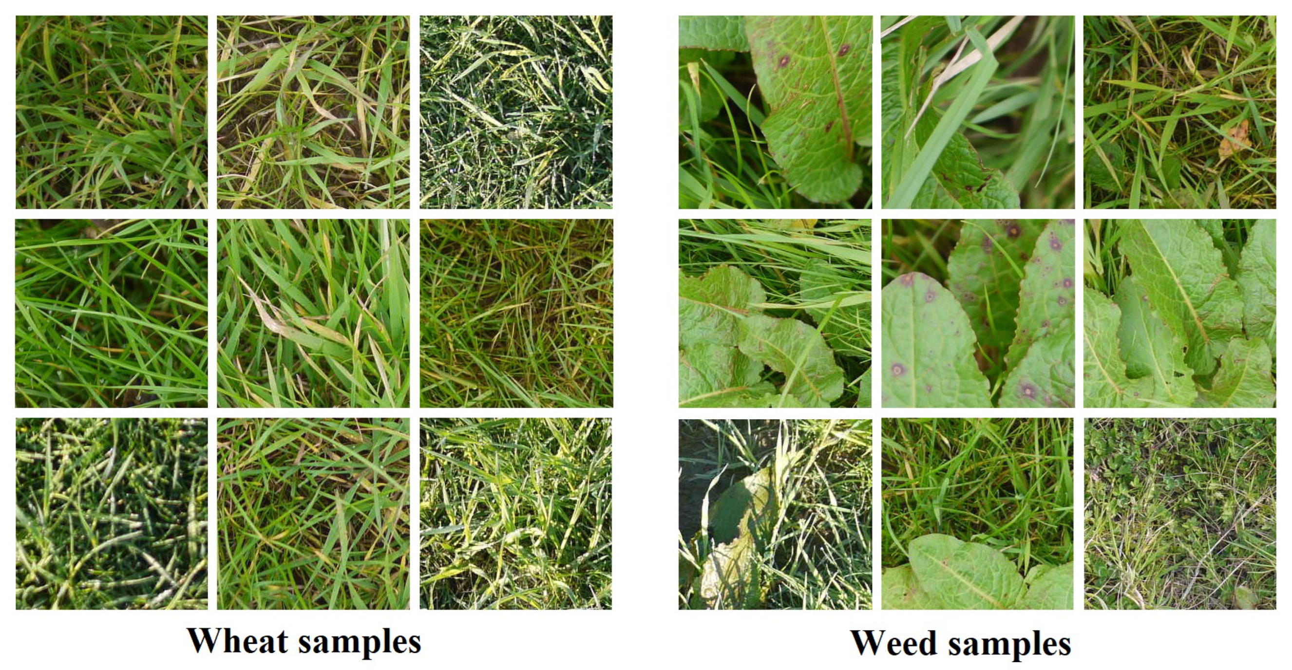
Figure 1.
Sample wheat and weed images in the employed dataset.
Figure 1.
Sample wheat and weed images in the employed dataset.
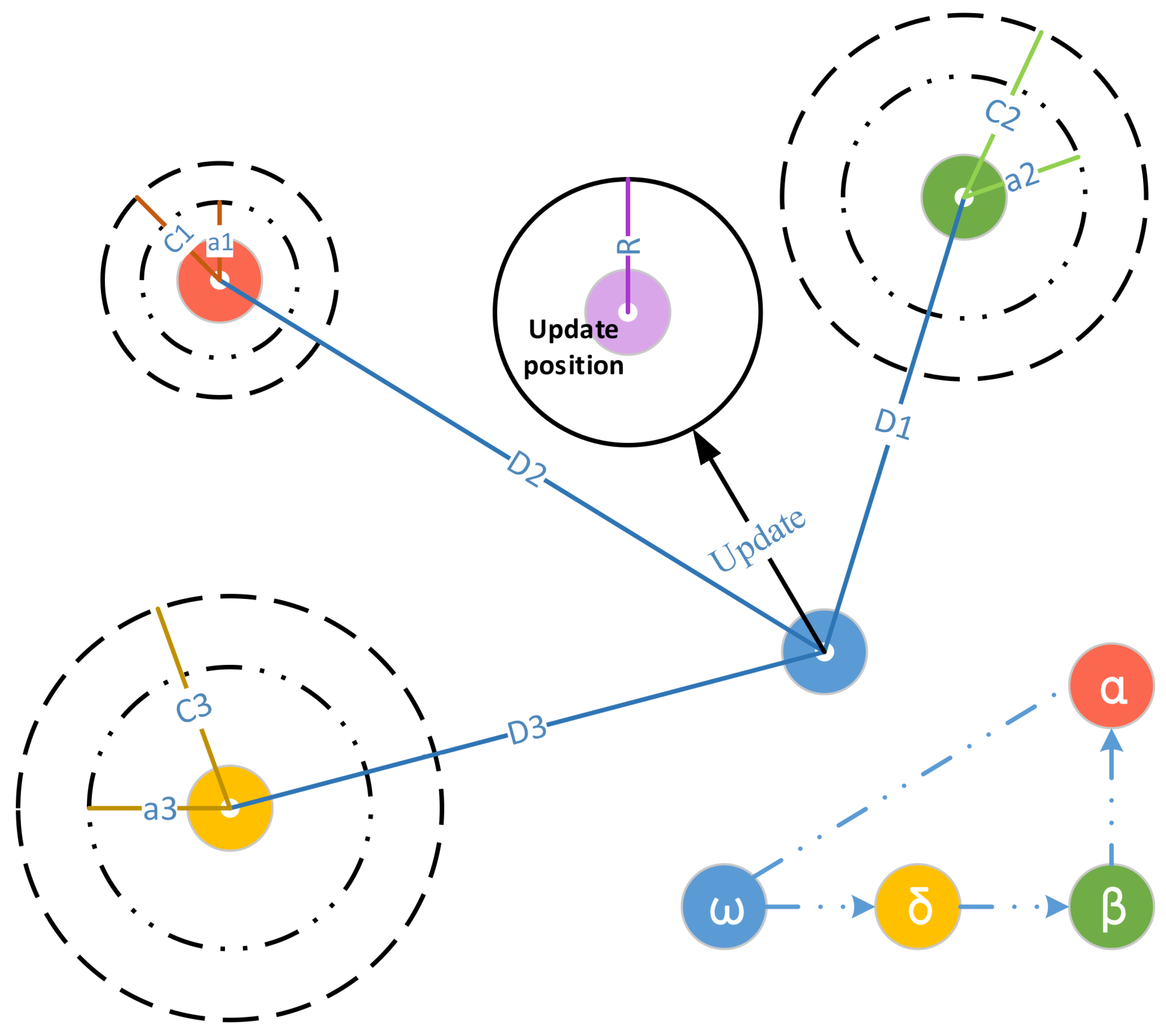
Figure 2.
The updating process of the grey wolf optimization algorithm.
Figure 2.
The updating process of the grey wolf optimization algorithm.
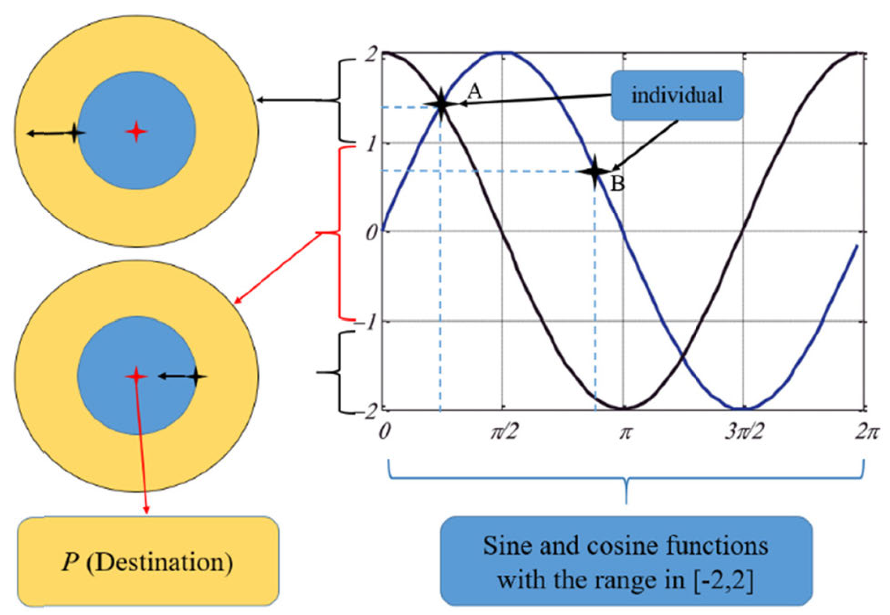
Figure 3.
Tolerance given to the solutions that proceed in either direction toward or away from the destination for sine and cosine functions [
41].
Figure 3.
Tolerance given to the solutions that proceed in either direction toward or away from the destination for sine and cosine functions [
41].
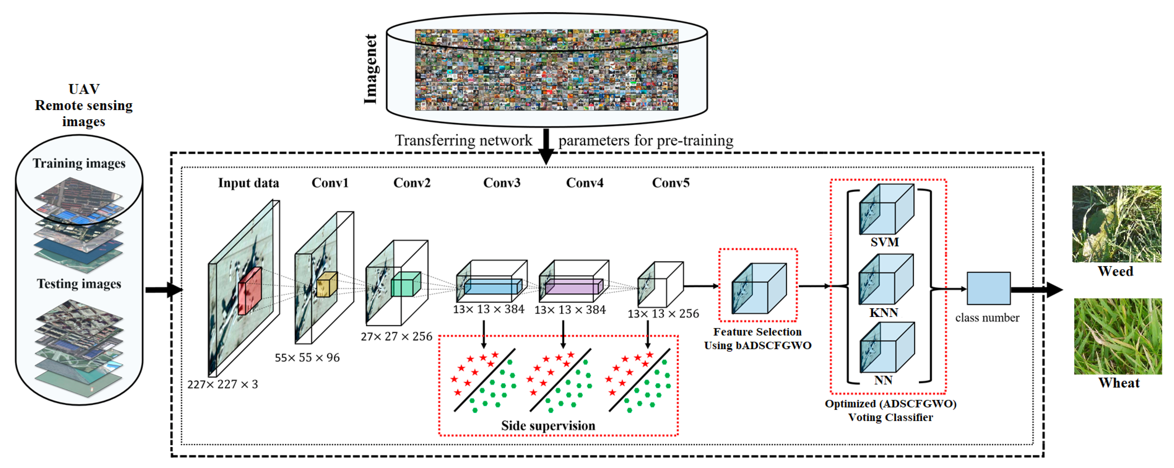
Figure 4.
The proposed methodology for weed/wheat classification.
Figure 4.
The proposed methodology for weed/wheat classification.
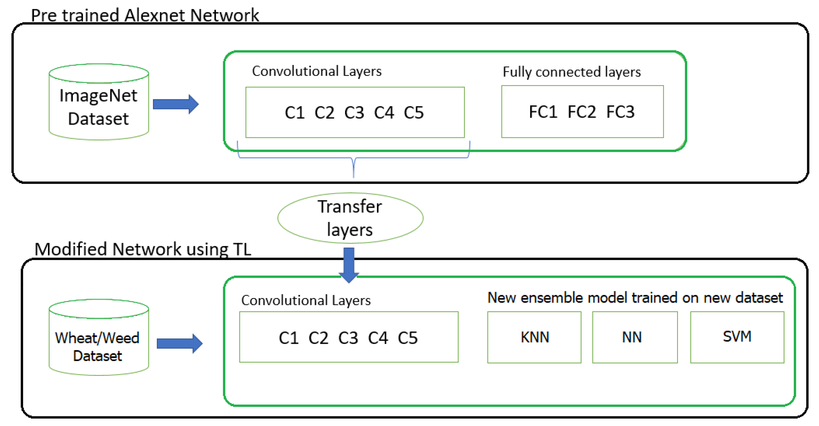
Figure 5.
The transfer learning process.
Figure 5.
The transfer learning process.
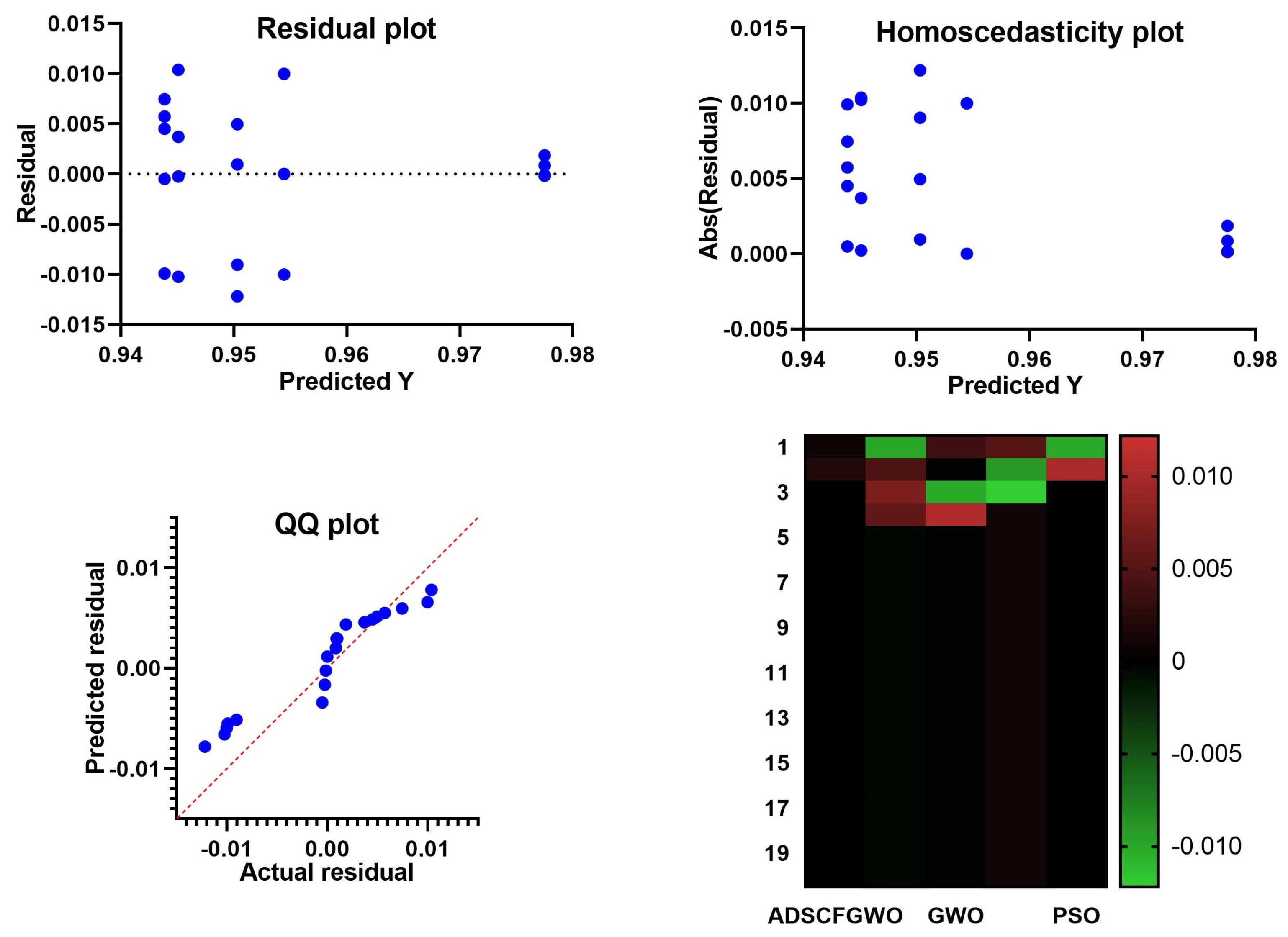
Figure 6.
Residual, homoscedasticity, and QQ plots and heatmap of the ADSCFGWO and compared algorithms.
Figure 6.
Residual, homoscedasticity, and QQ plots and heatmap of the ADSCFGWO and compared algorithms.
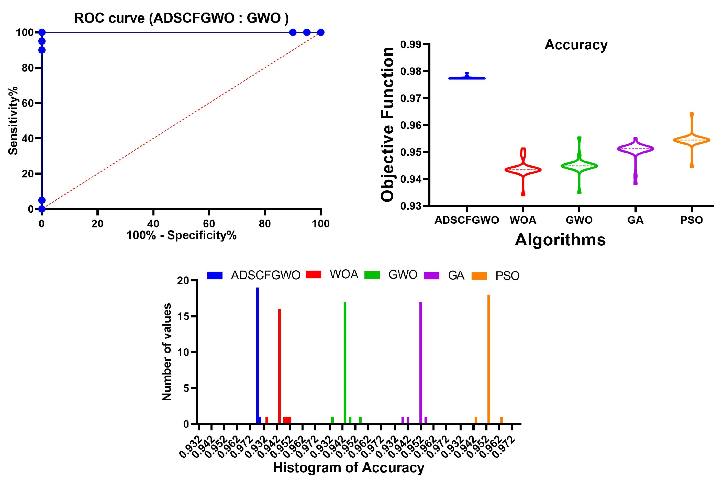
Figure 7.
ROC, accuracy, and histogram plots of the ADSCFGWO and compared algorithms.
Figure 7.
ROC, accuracy, and histogram plots of the ADSCFGWO and compared algorithms.
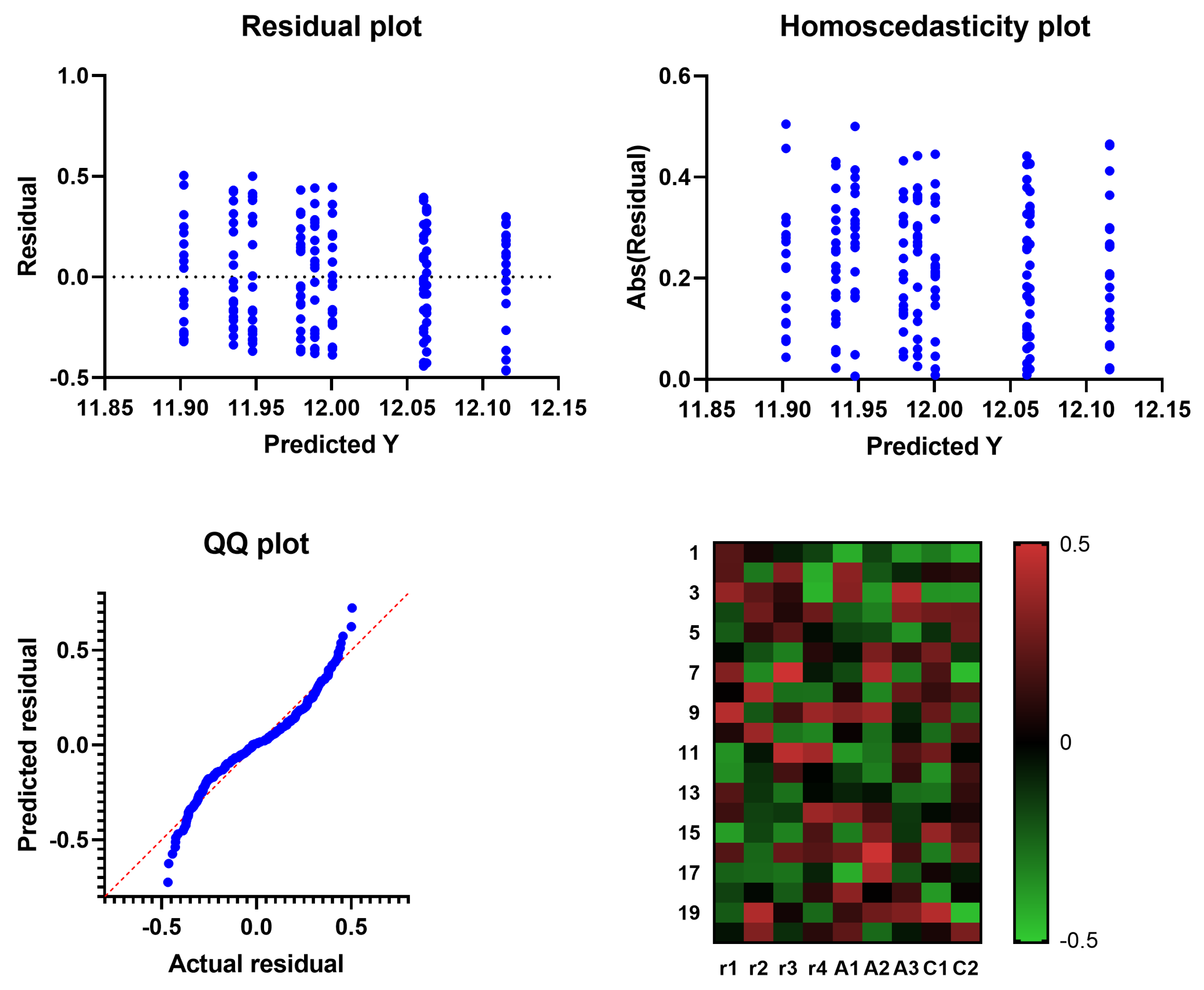
Figure 8.
Residual, homoscedasticity, and QQ plots and heatmap of ADSCFGWO’s parameters (, , , , , , , , and ) based on convergence time.
Figure 8.
Residual, homoscedasticity, and QQ plots and heatmap of ADSCFGWO’s parameters (, , , , , , , , and ) based on convergence time.
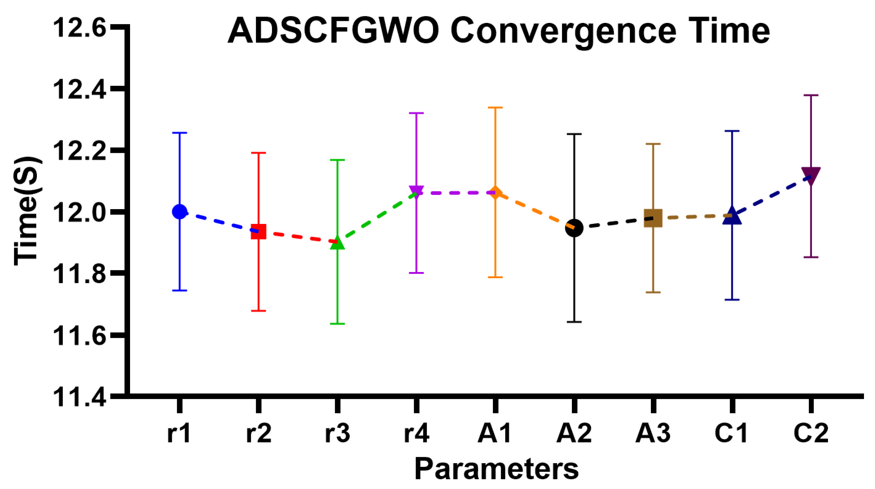
Figure 9.
Convergence time of ADSCFGWO’s parameters (, , , , , , , , and ).
Figure 9.
Convergence time of ADSCFGWO’s parameters (, , , , , , , , and ).
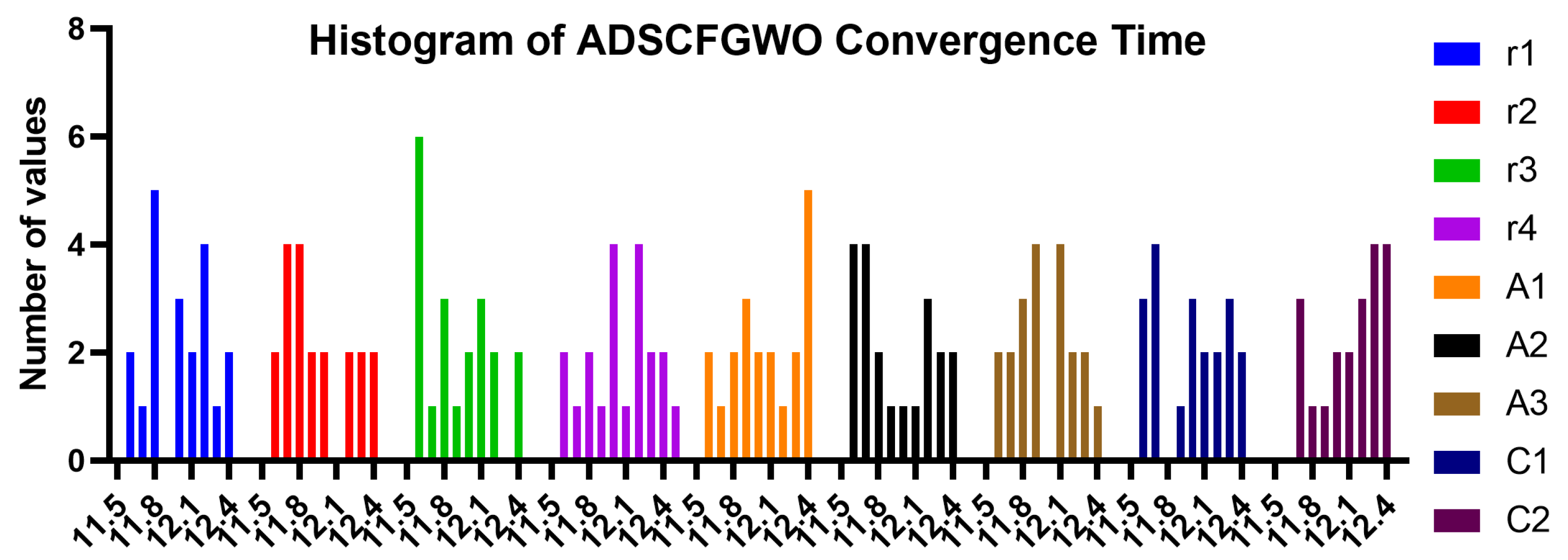
Figure 10.
Histogram of convergence time of ADSCFGWO’s parameters (, , , , , , , , and ).
Figure 10.
Histogram of convergence time of ADSCFGWO’s parameters (, , , , , , , , and ).
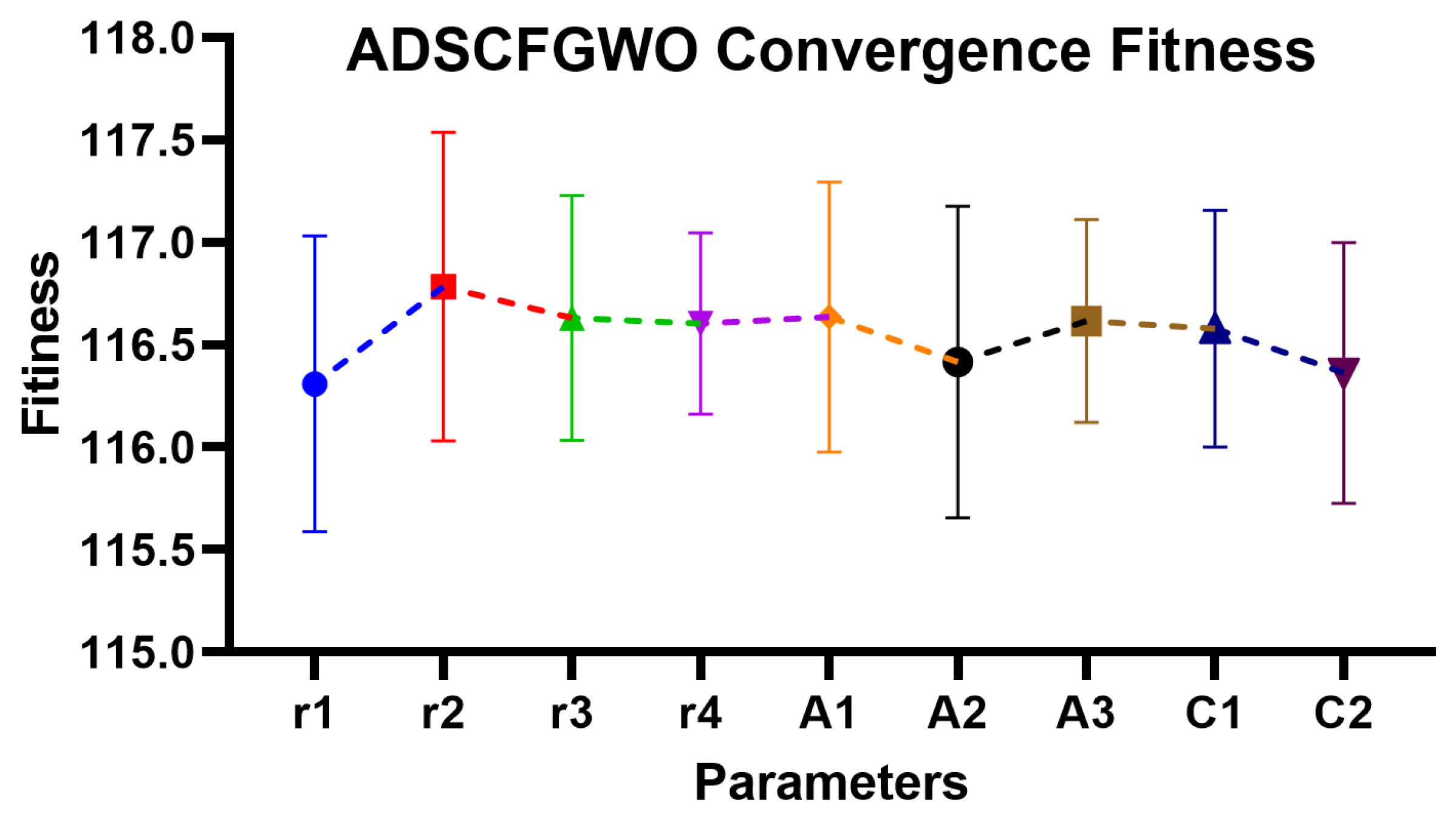
Figure 11.
Convergence fitness of ADSCFGWO’s parameters (, , , , , , , , and ).
Figure 11.
Convergence fitness of ADSCFGWO’s parameters (, , , , , , , , and ).
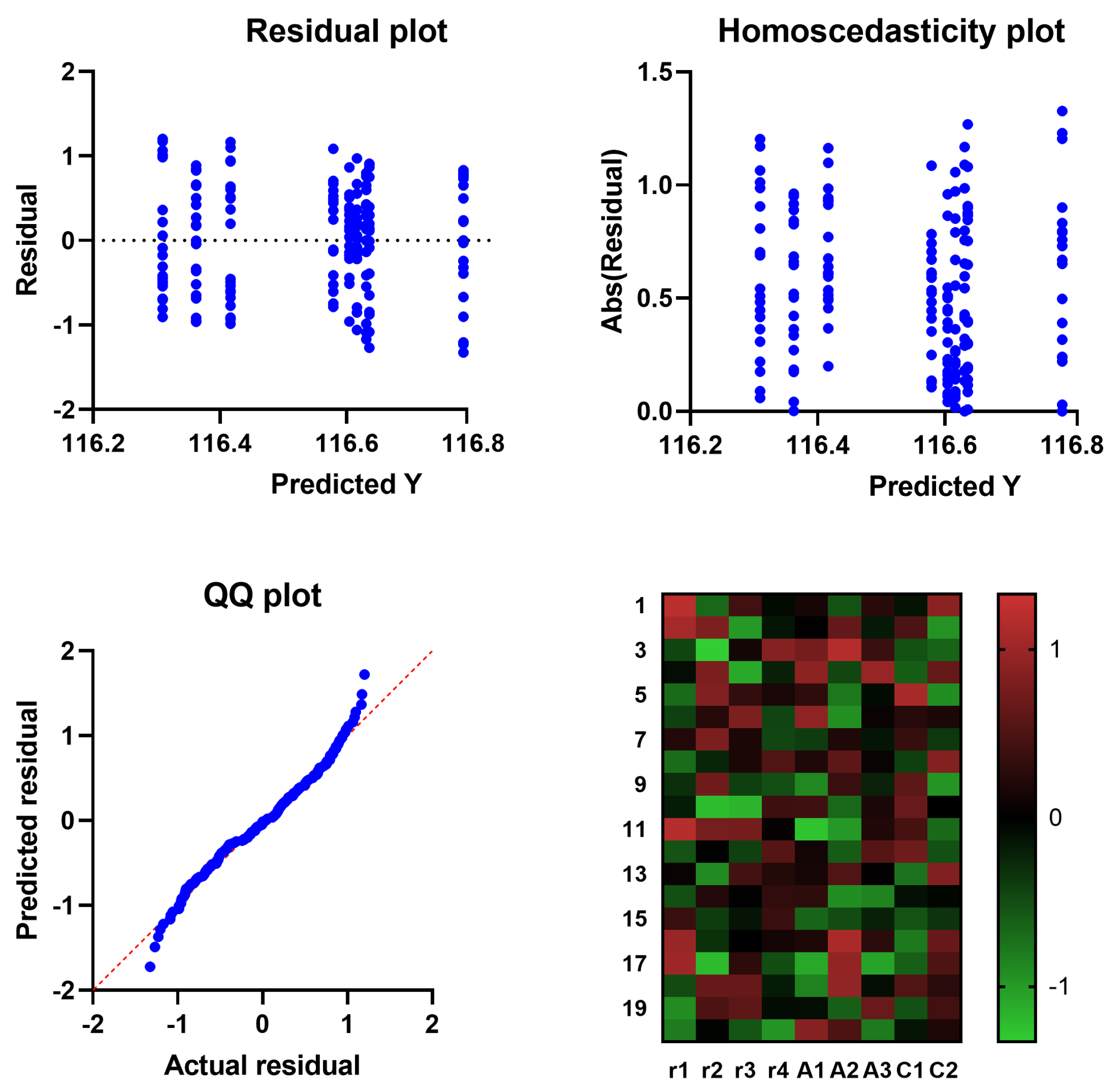
Figure 12.
Residual, homoscedasticity, and QQ plots and heatmap of ADSCFGWO’s parameters (, , , , , , , , and ) based on convergence fitness.
Figure 12.
Residual, homoscedasticity, and QQ plots and heatmap of ADSCFGWO’s parameters (, , , , , , , , and ) based on convergence fitness.
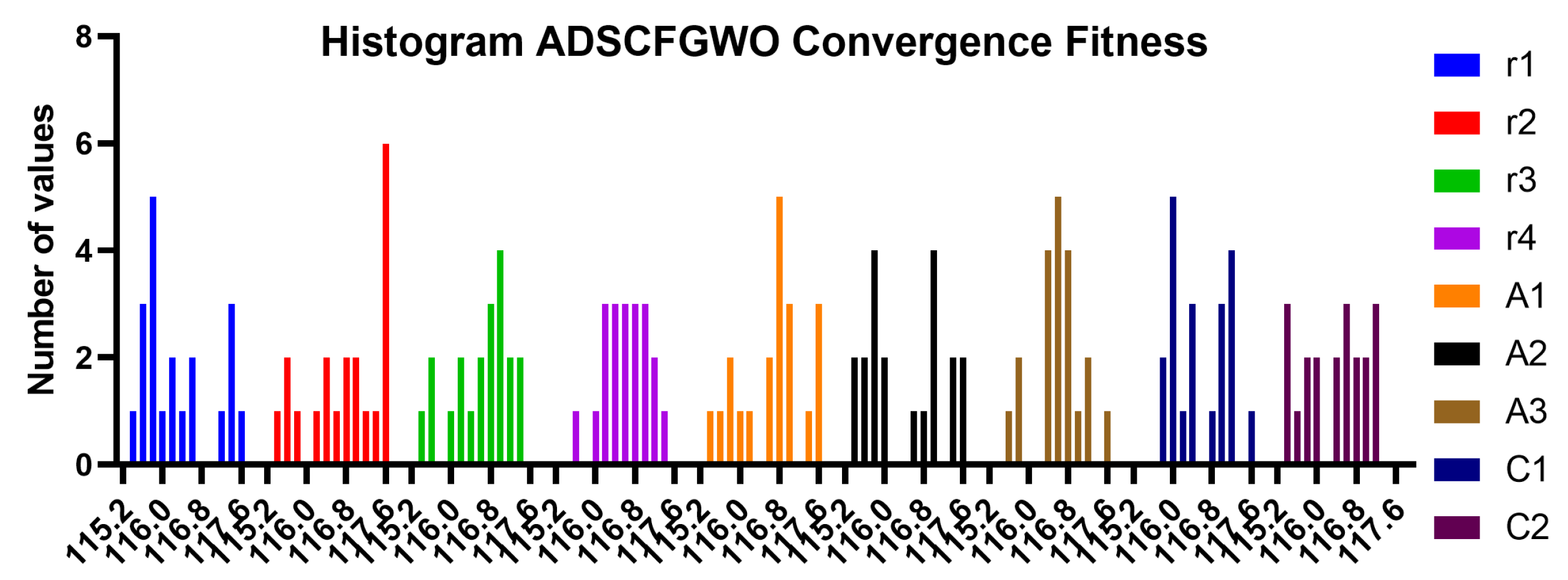
Figure 13.
Histogram of convergence fitness of ADSCFGWO’s parameters (, , , , , , , , and ).
Figure 13.
Histogram of convergence fitness of ADSCFGWO’s parameters (, , , , , , , , and ).
Table 1.
Weed detection approaches published in the literature.
Table 1.
Weed detection approaches published in the literature.
| Reference | Task | Target Crop | Model | Precision |
|---|
| [3] | Detection and classification of weeds | Unspecified | RF | 95% |
| [4] | Canopy structure measurement | Avocado tree | RF | 96% |
| [5] | Recognition of weed types | Maize | KNN, RF | 81%, 76.95% |
| [30] | Early weed mapping | Sunflower, cotton | RF | 87.90% |
| [31] | Weed detection by UAV | Maize | YOLOv3 | 98% |
| [24] | Water aquatic vegetation monitoring | Stratiotes aloides | RF | 92.19% |
| [25] | Mapping of land cover | 9 perennial crops | SVM | 84.80% |
| [26] | Recognition of weed types | 8 weed plants | SVM | 92.35% |
| [27] | Detection of weeds using shape feature | Sugar beet | SVM | 95% |
| [28] | Detection of weeds | Soybean | SVM | 95.07% |
| [32] | Weed detection using image processing | Chilli | RF | 96% |
| [33] | Mapping of weeds using images from UAV | Maize, Sunflower | SVM | 95.50% |
Table 2.
Configuration parameters of the proposed feature selection method.
Table 2.
Configuration parameters of the proposed feature selection method.
| Parameter | Value |
|---|
| Iterations | 100 |
| Agents | 10 |
| of Equation (20) | 0.99 |
| of Equation (20) | 0.01 |
| [0, 12] |
| a | [−10, 10] |
| b | [−10, 10] |
Table 3.
Configuration parameters of the optimization algorithms.
Table 3.
Configuration parameters of the optimization algorithms.
| Algorithm | Parameter | Value |
|---|
| GA | Cross over | 0.9 |
| | Agents | 10 |
| | Iterations | 80 |
| | Selection mechanism | Roulette wheel |
| | Mutation ratio | 0.1 |
| PSO | Acceleration constants | [2, 2] |
| | Iterations | 80 |
| | Inertia , | [0.6, 0.9] |
| | Particles | 10 |
| WOA | r | [0, 1] |
| | Whales | 10 |
| | Iterations | 80 |
| | a | 2 to 0 |
| GWO | a | 2 to 0 |
| | Iterations | 80 |
| | Wolves | 10 |
| FA | Iterations | 80 |
| | Fireflies | 10 |
Table 4.
Evaluation metrics used in assessing the feature selection approach.
Table 4.
Evaluation metrics used in assessing the feature selection approach.
| Metric | Formula |
|---|
| Average fitness size | |
| Average error | |
| Standard deviation | |
| Best fitness | |
| Worst fitness | |
| Mean | |
Table 5.
Evaluation metrics used in assessing the proposed optimized voting classifier.
Table 5.
Evaluation metrics used in assessing the proposed optimized voting classifier.
| Metric | Formula |
|---|
| F1-score | |
| Specificity (TNR) | |
| Accuracy | |
| Sensitivity (TPR) | |
| Nvalue (NPV) | |
| Pvalue (PPV) | |
Table 6.
Evaluation of three deep networks for feature extraction.
Table 6.
Evaluation of three deep networks for feature extraction.
| | VGGNet | ResNet-50 | AlexNet |
|---|
| Accuracy | 0.769 | 0.833 | 0.847 |
| Specificity (TNR) | 0.800 | 0.800 | 0.783 |
| Sensitivity (TPR) | 0.714 | 0.862 | 0.889 |
| Nvalue (NPV) | 0.833 | 0.833 | 0.818 |
| Pvalue (PPV) | 0.667 | 0.833 | 0.865 |
| F-score | 0.690 | 0.847 | 0.877 |
Table 7.
Evaluation of the proposed feature selection method and three other competing methods.
Table 7.
Evaluation of the proposed feature selection method and three other competing methods.
| | bADSCFGWO | bGWO | bGWO_PSO | bPSO | bWAO | bFA | bGA |
|---|
| Average select size | 0.647 | 0.847 | 0.981 | 0.847 | 1.011 | 0.882 | 0.790 |
| Std fitness | 0.580 | 0.585 | 0.603 | 0.584 | 0.586 | 0.621 | 0.586 |
| Average fitness | 0.758 | 0.774 | 0.782 | 0.772 | 0.780 | 0.824 | 0.785 |
| Average error | 0.695 | 0.712 | 0.751 | 0.746 | 0.745 | 0.744 | 0.725 |
| Worst fitness | 0.758 | 0.761 | 0.846 | 0.820 | 0.820 | 0.841 | 0.804 |
| Best fitness | 0.660 | 0.694 | 0.736 | 0.753 | 0.744 | 0.743 | 0.689 |
Table 8.
Evaluating the results achieved by three baseline machine learning models.
Table 8.
Evaluating the results achieved by three baseline machine learning models.
| | KNN | SVM | NN |
|---|
| Accuracy | 0.891 | 0.921 | 0.935 |
| Specificity (TNR) | 0.743 | 0.857 | 0.870 |
| Sensitivity (TPR) | 0.952 | 0.952 | 0.971 |
| Nvalue (NPV) | 0.867 | 0.900 | 0.943 |
| Pvalue (PPV) | 0.899 | 0.930 | 0.930 |
| F-score | 0.925 | 0.941 | 0.950 |
Table 9.
Evaluation of the results achieved by optimizing the proposed voting classifier using the proposed optimization method and three other optimizers.
Table 9.
Evaluation of the results achieved by optimizing the proposed voting classifier using the proposed optimization method and three other optimizers.
| | Voting (ADSCFGWO) | Voting (WOA) | Voting (GWO) | Voting (GA) | Voting (PSO) |
|---|
| Accuracy | 0.977 | 0.943 | 0.945 | 0.951 | 0.954 |
| Specificity (TNR) | 0.952 | 0.870 | 0.870 | 0.870 | 0.870 |
| Sensitivity (TPR) | 0.984 | 0.977 | 0.977 | 0.981 | 0.983 |
| Nvalue (NPV) | 0.943 | 0.943 | 0.943 | 0.943 | 0.943 |
| Pvalue (PPV) | 0.987 | 0.943 | 0.945 | 0.954 | 0.958 |
| F-score | 0.986 | 0.960 | 0.961 | 0.967 | 0.970 |
Table 10.
Statistical analysis of the achieved classification results using the proposed optimized voting ensemble model.
Table 10.
Statistical analysis of the achieved classification results using the proposed optimized voting ensemble model.
| | ADSCFGWO | WOA | GWO | GA | PSO |
|---|
| Number of values | 20 | 20 | 20 | 20 | 20 |
| 25% Percentile | 0.9774 | 0.943 | 0.945 | 0.951 | 0.954 |
| 75% Percentile | 0.9774 | 0.943 | 0.945 | 0.951 | 0.954 |
| Std. error of mean | 0.0001 | 0.001 | 0.001 | 0.001 | 0.001 |
| Std. deviation | 0.0004 | 0.003 | 0.003 | 0.004 | 0.003 |
| Mean | 0.9775 | 0.9439 | 0.945 | 0.950 | 0.954 |
| Minimum | 0.9774 | 0.934 | 0.935 | 0.938 | 0.944 |
| Maximum | 0.9794 | 0.951 | 0.956 | 0.955 | 0.964 |
| Median | 0.9774 | 0.943 | 0.945 | 0.951 | 0.954 |
| Range | 0.002 | 0.017 | 0.021 | 0.0172 | 0.020 |
| Upper 95% CI of mean | 0.9777 | 0.945 | 0.947 | 0.952 | 0.956 |
| Lower 95% CI of mean | 0.9773 | 0.942 | 0.944 | 0.949 | 0.953 |
| Coefficient of variation | 0.0501% | 0.353% | 0.366% | 0.397% | 0.340% |
| Geometric SD factor | 1.001 | 1.004 | 1.004 | 1.004 | 1.003 |
| Geometric mean | 0.9775 | 0.944 | 0.945 | 0.950 | 0.954 |
| Upper 95% CI of harm. mean | 0.9777 | 0.945 | 0.947 | 0.952 | 0.956 |
| Lower 95% CI of harm. mean | 0.9773 | 0.942 | 0.944 | 0.949 | 0.953 |
| Sum | 19.55 | 18.88 | 18.90 | 19.01 | 19.09 |
Table 11.
ANOVA test of the achieved classification results using the optimized voting ensemble model.
Table 11.
ANOVA test of the achieved classification results using the optimized voting ensemble model.
| | SS | DF | MS | F (DFn, DFd) | p Value |
|---|
| Treatment | 0.01496 | 4 | 0.003739 | F (4, 95) = 389.0 | p < 0.0001 |
| Residual | 0.0009132 | 95 | 0.000009612 | | |
| Total | 0.01587 | 99 | | | |
Table 12.
Wilcoxon signed-rank test of the results achieved by the proposed optimized voting classifier.
Table 12.
Wilcoxon signed-rank test of the results achieved by the proposed optimized voting classifier.
| | ADSCFGWO | WOA | GWO | GA | PSO |
|---|
| Theoretical median | 0 | 0 | 0 | 0 | 0 |
| Actual median | 0.9774 | 0.9434 | 0.9449 | 0.9513 | 0.9544 |
| Number of values | 20 | 20 | 20 | 20 | 20 |
| Wilcoxon signed-rank test | | | | | |
| p value (two-tailed) | <0.0001 | <0.0001 | <0.0001 | <0.0001 | <0.0001 |
| Sum of positive ranks | 210 | 210 | 210 | 210 | 210 |
| Sum of signed ranks (W) | 210 | 210 | 210 | 210 | 210 |
| Sum of negative ranks | 0 | 0 | 0 | 0 | 0 |
| Exact or estimate? | Exact | Exact | Exact | Exact | Exact |
| p value summary | **** | **** | **** | **** | **** |
| Discrepancy | 0.9774 | 0.9434 | 0.9449 | 0.9513 | 0.9544 |
| Significant (alpha = 0.05)? | Yes | Yes | Yes | Yes | Yes |
Table 13.
Convergence time results (in seconds) for different values of ADSCFGWO’s parameters (1).
Table 13.
Convergence time results (in seconds) for different values of ADSCFGWO’s parameters (1).
| | | |
|---|
| Values | Time | Values | Time | Values | Time | Values | Time |
| 0.05 | 12.21 | 0.05 | 11.99 | 0.05 | 11.82 | 0.05 | 11.89 |
| 0.10 | 12.21 | 0.10 | 11.64 | 0.10 | 12.21 | 0.10 | 11.63 |
| 0.15 | 12.36 | 0.15 | 12.15 | 0.15 | 12.01 | 0.15 | 11.61 |
| 0.20 | 11.82 | 0.20 | 12.20 | 0.20 | 11.98 | 0.20 | 12.32 |
| 0.25 | 11.77 | 0.25 | 12.04 | 0.25 | 12.12 | 0.25 | 12.02 |
| 0.30 | 11.98 | 0.30 | 11.73 | 0.30 | 11.59 | 0.30 | 12.15 |
| 0.35 | 12.31 | 0.35 | 11.59 | 0.35 | 12.40 | 0.35 | 12.00 |
| 0.40 | 12.00 | 0.40 | 12.35 | 0.40 | 11.63 | 0.40 | 11.78 |
| 0.45 | 12.44 | 0.45 | 11.72 | 0.45 | 12.06 | 0.45 | 12.44 |
| 0.50 | 12.07 | 0.50 | 12.31 | 0.50 | 11.61 | 0.50 | 11.73 |
| 0.55 | 11.64 | 0.55 | 11.88 | 0.55 | 12.35 | 0.55 | 12.45 |
| 0.60 | 11.65 | 0.60 | 11.81 | 0.60 | 12.06 | 0.60 | 12.05 |
| 0.65 | 12.20 | 0.65 | 11.80 | 0.65 | 11.62 | 0.65 | 12.04 |
| 0.70 | 12.14 | 0.70 | 11.77 | 0.70 | 11.76 | 0.70 | 12.44 |
| 0.75 | 11.61 | 0.75 | 11.76 | 0.75 | 11.58 | 0.75 | 12.24 |
| 0.80 | 12.20 | 0.80 | 11.68 | 0.80 | 12.15 | 0.80 | 12.26 |
| 0.85 | 11.76 | 0.85 | 11.67 | 0.85 | 11.62 | 0.85 | 11.97 |
| 0.90 | 11.83 | 0.90 | 11.91 | 0.90 | 11.68 | 0.90 | 12.16 |
| 0.95 | 11.78 | 0.95 | 12.36 | 0.95 | 11.94 | 0.95 | 11.80 |
| 1.00 | 11.95 | 1.00 | 12.25 | 1.00 | 11.79 | 1.00 | 12.15 |
Table 14.
Convergence time results (in seconds) for different values of ADSCFGWO’s parameters (2).
Table 14.
Convergence time results (in seconds) for different values of ADSCFGWO’s parameters (2).
| | | | |
|---|
| Values | Time | Values | Time | Values | Time | Values | Time | Values | Time |
| 0.05 | 11.63 | 0.10 | 11.78 | 0.10 | 11.60 | 0.10 | 11.68 | 0.10 | 11.70 |
| 0.10 | 12.40 | 0.20 | 11.73 | 0.20 | 11.88 | 0.20 | 12.06 | 0.20 | 12.21 |
| 0.15 | 12.39 | 0.30 | 11.58 | 0.30 | 12.41 | 0.30 | 11.62 | 0.30 | 11.75 |
| 0.20 | 11.83 | 0.40 | 11.63 | 0.40 | 12.30 | 0.40 | 12.26 | 0.40 | 12.37 |
| 0.25 | 11.90 | 0.50 | 11.77 | 0.50 | 11.62 | 0.50 | 11.87 | 0.50 | 12.38 |
| 0.30 | 12.02 | 0.60 | 12.24 | 0.60 | 12.11 | 0.60 | 12.27 | 0.60 | 11.98 |
| 0.35 | 11.88 | 0.70 | 12.36 | 0.70 | 11.67 | 0.70 | 12.17 | 0.70 | 11.65 |
| 0.40 | 12.12 | 0.80 | 11.61 | 0.80 | 12.21 | 0.80 | 12.11 | 0.80 | 12.32 |
| 0.45 | 12.38 | 0.90 | 12.32 | 0.90 | 11.88 | 0.90 | 12.24 | 0.90 | 11.85 |
| 0.50 | 12.08 | 1.00 | 11.67 | 1.00 | 11.93 | 1.00 | 11.72 | 1.00 | 12.32 |
| 0.55 | 11.69 | 1.10 | 11.66 | 1.10 | 12.17 | 1.10 | 12.26 | 1.10 | 12.09 |
| 0.60 | 11.90 | 1.20 | 11.64 | 1.20 | 12.10 | 1.20 | 11.63 | 1.20 | 12.27 |
| 0.65 | 11.97 | 1.30 | 11.89 | 1.30 | 11.71 | 1.30 | 11.70 | 1.30 | 12.23 |
| 0.70 | 12.39 | 1.40 | 12.10 | 1.40 | 11.84 | 1.40 | 11.96 | 1.40 | 12.18 |
| 0.75 | 11.75 | 1.50 | 12.24 | 1.50 | 11.84 | 1.50 | 12.35 | 1.50 | 12.29 |
| 0.80 | 12.33 | 1.60 | 12.44 | 1.60 | 12.14 | 1.60 | 11.68 | 1.60 | 12.41 |
| 0.85 | 11.63 | 1.70 | 12.34 | 1.70 | 11.77 | 1.70 | 12.03 | 1.70 | 12.04 |
| 0.90 | 12.40 | 1.80 | 11.95 | 1.80 | 12.12 | 1.80 | 11.61 | 1.80 | 12.13 |
| 0.95 | 12.19 | 1.90 | 12.21 | 1.90 | 12.29 | 1.90 | 12.43 | 1.90 | 11.65 |
| 1.00 | 12.29 | 2.00 | 11.68 | 2.00 | 11.92 | 2.00 | 12.04 | 2.00 | 12.41 |
Table 15.
Minimization results for different values of ADSCFGWO’s parameters (1).
Table 15.
Minimization results for different values of ADSCFGWO’s parameters (1).
| | | |
|---|
| Values | Fitness | Values | Fitness | Values | Fitness | Values | Fitness |
| 0.05 | 117.51 | 0.05 | 116.11 | 0.05 | 117.04 | 0.05 | 116.53 |
| 0.10 | 117.37 | 0.10 | 117.58 | 0.10 | 115.64 | 0.10 | 116.46 |
| 0.15 | 115.86 | 0.15 | 115.45 | 0.15 | 116.76 | 0.15 | 117.46 |
| 0.20 | 116.21 | 0.20 | 117.57 | 0.20 | 115.54 | 0.20 | 116.39 |
| 0.25 | 115.61 | 0.25 | 117.61 | 0.25 | 116.95 | 0.25 | 116.76 |
| 0.30 | 115.89 | 0.30 | 117.02 | 0.30 | 117.42 | 0.30 | 116.16 |
| 0.35 | 116.52 | 0.35 | 117.57 | 0.35 | 116.80 | 0.35 | 116.15 |
| 0.40 | 115.60 | 0.40 | 116.54 | 0.40 | 116.81 | 0.40 | 117.11 |
| 0.45 | 116.00 | 0.45 | 117.51 | 0.45 | 116.21 | 0.45 | 116.09 |
| 0.50 | 116.13 | 0.50 | 115.55 | 0.50 | 115.46 | 0.50 | 116.99 |
| 0.55 | 117.47 | 0.55 | 117.54 | 0.55 | 117.38 | 0.55 | 116.64 |
| 0.60 | 115.76 | 0.60 | 116.78 | 0.60 | 116.21 | 0.60 | 117.15 |
| 0.65 | 116.36 | 0.65 | 115.88 | 0.65 | 117.05 | 0.65 | 116.83 |
| 0.70 | 115.80 | 0.70 | 117.00 | 0.70 | 116.63 | 0.70 | 116.90 |
| 0.75 | 116.67 | 0.75 | 116.39 | 0.75 | 116.49 | 0.75 | 116.97 |
| 0.80 | 117.29 | 0.80 | 116.46 | 0.80 | 116.62 | 0.80 | 116.72 |
| 0.85 | 117.32 | 0.85 | 115.57 | 0.85 | 116.92 | 0.85 | 116.10 |
| 0.90 | 115.82 | 0.90 | 117.43 | 0.90 | 117.28 | 0.90 | 116.42 |
| 0.95 | 115.40 | 0.95 | 117.28 | 0.95 | 117.22 | 0.95 | 116.52 |
| 1.00 | 115.50 | 1.00 | 116.75 | 1.00 | 116.08 | 1.00 | 115.64 |
Table 16.
Minimization results for different values of ADSCFGWO’s parameters (2).
Table 16.
Minimization results for different values of ADSCFGWO’s parameters (2).
| | | | |
|---|
| Values | Fitness | Values | Fitness | Values | Fitness | Values | Fitness | Values | Fitness |
| 0.05 | 116.77 | 0.10 | 115.88 | 0.10 | 116.87 | 0.10 | 116.45 | 0.10 | 117.25 |
| 0.10 | 116.62 | 0.20 | 117.05 | 0.20 | 116.45 | 0.20 | 117.06 | 0.20 | 115.41 |
| 0.15 | 117.38 | 0.30 | 117.58 | 0.30 | 116.97 | 0.30 | 116.05 | 0.30 | 115.71 |
| 0.20 | 117.53 | 0.40 | 115.96 | 0.40 | 117.58 | 0.40 | 115.97 | 0.40 | 117.01 |
| 0.25 | 116.93 | 0.50 | 115.64 | 0.50 | 116.53 | 0.50 | 117.66 | 0.50 | 115.44 |
| 0.30 | 117.54 | 0.60 | 115.48 | 0.60 | 116.67 | 0.60 | 116.82 | 0.60 | 116.53 |
| 0.35 | 116.24 | 0.70 | 116.61 | 0.70 | 116.47 | 0.70 | 116.93 | 0.70 | 115.99 |
| 0.40 | 116.83 | 0.80 | 117.02 | 0.80 | 116.67 | 0.80 | 116.16 | 0.80 | 117.20 |
| 0.45 | 115.75 | 0.90 | 116.78 | 0.90 | 116.39 | 0.90 | 117.17 | 0.90 | 115.40 |
| 0.50 | 117.03 | 1.00 | 115.74 | 1.00 | 116.78 | 1.00 | 117.24 | 1.00 | 116.36 |
| 0.55 | 115.36 | 1.10 | 115.43 | 1.10 | 116.82 | 1.10 | 117.02 | 1.10 | 115.67 |
| 0.60 | 116.75 | 1.20 | 115.82 | 1.20 | 117.17 | 1.20 | 117.28 | 1.20 | 115.84 |
| 0.65 | 116.77 | 1.30 | 116.93 | 1.30 | 116.63 | 1.30 | 115.83 | 1.30 | 117.19 |
| 0.70 | 116.93 | 1.40 | 115.50 | 1.40 | 115.76 | 1.40 | 116.47 | 1.40 | 116.32 |
| 0.75 | 115.98 | 1.50 | 115.92 | 1.50 | 116.40 | 1.50 | 116.04 | 1.50 | 116.02 |
| 0.80 | 116.82 | 1.60 | 117.51 | 1.60 | 116.88 | 1.60 | 115.79 | 1.60 | 117.02 |
| 0.85 | 115.55 | 1.70 | 117.36 | 1.70 | 115.55 | 1.70 | 115.96 | 1.70 | 116.86 |
| 0.90 | 115.79 | 1.80 | 117.35 | 1.80 | 116.52 | 1.80 | 117.10 | 1.80 | 116.63 |
| 0.95 | 116.55 | 1.90 | 115.80 | 1.90 | 117.28 | 1.90 | 116.05 | 1.90 | 116.78 |
| 1.00 | 117.50 | 2.00 | 116.91 | 2.00 | 115.82 | 2.00 | 116.44 | 2.00 | 116.54 |
Table 17.
ANOVA test analyzing the convergence time.
Table 17.
ANOVA test analyzing the convergence time.
| | SS | DF | MS | F (DFn, DFd) | p Value |
|---|
| Treatment | 0.7603 | 8 | 0.09504 | F (8, 171) = 1.336 | p = 0.002288 |
| Residual | 12.17 | 171 | 0.07115 | | |
| Total | 12.93 | 179 | | | |
Table 18.
Wilcoxon signed-rank test of the convergence time.
Table 18.
Wilcoxon signed-rank test of the convergence time.
| | | | | | | | | | |
|---|
| Number of values | 20 | 20 | 20 | 20 | 20 | 20 | 20 | 20 | 20 |
| Actual mean | 12 | 11.94 | 11.9 | 12.06 | 12.06 | 11.95 | 11.98 | 11.99 | 12.12 |
| Theoretical mean | 0 | 0 | 0 | 0 | 0 | 0 | 0 | 0 | 0 |
| df | df = 19 | df = 19 | df = 19 | df = 19 | df = 19 | df = 19 | df = 19 | df = 19 | df = 19 |
| t | t = 209.6 | t = 208.2 | t = 200.1 | t = 207.8 | t = 196.0 | t = 175.3 | t = 222.7 | t = 195.7 | t = 205.8 |
| p value (two-tailed) | <0.0001 | <0.0001 | <0.0001 | <0.0001 | <0.0001 | <0.0001 | <0.0001 | <0.0001 | <0.0001 |
| Discrepancy | 12 | 11.94 | 11.9 | 12.06 | 12.06 | 11.95 | 11.98 | 11.99 | 12.12 |
| Significant (alpha = 0.05)? | Yes | Yes | Yes | Yes | Yes | Yes | Yes | Yes | Yes |
| SEM of discrepancy | 0.0572 | 0.0573 | 0.0594 | 0.0580 | 0.0615 | 0.0681 | 0.0538 | 0.0612 | 0.0588 |
| SD of discrepancy | 0.2561 | 0.2564 | 0.266 | 0.2596 | 0.2752 | 0.3048 | 0.2406 | 0.2739 | 0.2633 |
| R squared | 0.9996 | 0.9996 | 0.9995 | 0.9996 | 0.9995 | 0.9994 | 0.9996 | 0.9995 | 0.9996 |
| 95% confidence (From) | 11.88 | 11.82 | 11.78 | 11.94 | 11.93 | 11.81 | 11.87 | 11.86 | 11.99 |
| 95% confidence (To) | 12.12 | 12.06 | 12.03 | 12.18 | 12.19 | 12.09 | 12.09 | 12.12 | 12.24 |
Table 19.
Statistical analysis of the convergence time.
Table 19.
Statistical analysis of the convergence time.
| | | | | | | | | | |
|---|
| Number of values | 20 | 20 | 20 | 20 | 20 | 20 | 20 | 20 | 20 |
| Minimum | 11.61 | 11.6 | 11.58 | 11.62 | 11.64 | 11.58 | 11.61 | 11.61 | 11.65 |
| Range | 0.830 | 0.760 | 0.820 | 0.830 | 0.760 | 0.860 | 0.800 | 0.820 | 0.760 |
| 25% Percentile | 11.78 | 11.73 | 11.62 | 11.83 | 11.85 | 11.67 | 11.79 | 11.69 | 11.88 |
| 75% Percentile | 12.21 | 12.19 | 12.11 | 12.26 | 12.37 | 12.25 | 12.17 | 12.26 | 12.32 |
| Mean | 12.0 | 11.94 | 11.90 | 12.06 | 12.06 | 11.95 | 11.98 | 11.99 | 12.12 |
| Median | 11.99 | 11.85 | 11.89 | 12.05 | 12.05 | 11.84 | 11.93 | 12.04 | 12.20 |
| Maximum | 12.45 | 12.37 | 12.41 | 12.46 | 12.41 | 12.45 | 12.41 | 12.43 | 12.42 |
| Std. error of mean | 0.057 | 0.057 | 0.059 | 0.058 | 0.061 | 0.068 | 0.053 | 0.061 | 0.058 |
| Std. deviation | 0.256 | 0.256 | 0.266 | 0.259 | 0.275 | 0.304 | 0.240 | 0.273 | 0.263 |
| Sum | 240.0 | 238.7 | 238.0 | 241.2 | 241.3 | 239.0 | 239.6 | 239.8 | 242.3 |
Table 20.
Wilcoxon signed-rank test of the fitness of the proposed ADSCFGWO algorithm.
Table 20.
Wilcoxon signed-rank test of the fitness of the proposed ADSCFGWO algorithm.
| | | | | | | | | | |
|---|
| Number of values | 20 | 20 | 20 | 20 | 20 | 20 | 20 | 20 | 20 |
| Actual mean | 116.3 | 116.8 | 116.6 | 116.6 | 116.6 | 116.4 | 116.6 | 116.6 | 116.4 |
| Theoretical mean | 0 | 0 | 0 | 0 | 0 | 0 | 0 | 0 | 0 |
| df | df = 19 | df = 19 | df = 19 | df = 19 | df = 19 | df = 19 | df = 19 | df = 19 | df = 19 |
| t | t = 721.8 | t = 694.1 | t = 872.0 | t = 1178 | t = 791.3 | t = 685.0 | t = 1051 | t = 903.7 | t = 818.3 |
| Discrepancy | 116.3 | 116.8 | 116.6 | 116.6 | 116.6 | 116.4 | 116.6 | 116.6 | 116.4 |
| p value (two-tailed) | <0.0001 | <0.0001 | <0.0001 | <0.0001 | <0.0001 | <0.0001 | <0.0001 | <0.0001 | <0.0001 |
| Significant (alpha = 0.05)? | Yes | Yes | Yes | Yes | Yes | Yes | Yes | Yes | Yes |
| SEM of discrepancy | 0.1611 | 0.1683 | 0.1337 | 0.09896 | 0.1474 | 0.1699 | 0.1109 | 0.129 | 0.1422 |
| SD of discrepancy | 0.7206 | 0.7525 | 0.5981 | 0.4426 | 0.6592 | 0.76 | 0.496 | 0.5769 | 0.6359 |
| R squared | 1 | 1 | 1 | 1 | 1 | 1 | 1 | 1 | 1 |
| 95% confidence (from) | 116.0 | 116.4 | 116.4 | 116.4 | 116.3 | 116.1 | 116.4 | 116.3 | 116.1 |
| 95% confidence (to) | 116.6 | 117.1 | 116.9 | 116.8 | 116.9 | 116.8 | 116.8 | 116.8 | 116.7 |
Table 21.
ANOVA test of the fitness of the proposed ADSCFGWO algorithm.
Table 21.
ANOVA test of the fitness of the proposed ADSCFGWO algorithm.
| | SS | DF | MS | F (DFn, DFd) | p Value |
|---|
| Treatment | 3.749 | 8 | 0.4686 | F (8, 171) = 1.160 | p = 0.003259 |
| Residual | 69.05 | 171 | 0.4038 | | |
| Total | 72.8 | 179 | | | |
Table 22.
Statistical analysis of the fitness achieved by the proposed optimization algorithm.
Table 22.
Statistical analysis of the fitness achieved by the proposed optimization algorithm.
| | | | | | | | | | |
|---|
| Number of values | 20 | 20 | 20 | 20 | 20 | 20 | 20 | 20 | 20 |
| Range | 2.108 | 2.158 | 1.967 | 1.824 | 2.176 | 2.148 | 2.029 | 1.87 | 1.851 |
| 25% Percentile | 115.8 | 116.2 | 116.2 | 116.2 | 116.1 | 115.8 | 116.4 | 116.0 | 115.7 |
| 75% Percentile | 117.1 | 117.5 | 117.1 | 117.0 | 117.0 | 117.0 | 116.9 | 117.1 | 117.0 |
| Minimum | 115.4 | 115.5 | 115.5 | 115.6 | 115.4 | 115.4 | 115.6 | 115.8 | 115.4 |
| Mean | 116.3 | 116.8 | 116.6 | 116.6 | 116.6 | 116.4 | 116.6 | 116.6 | 116.4 |
| Median | 116.1 | 116.9 | 116.8 | 116.6 | 116.8 | 116.3 | 116.7 | 116.5 | 116.4 |
| Maximum | 117.5 | 117.6 | 117.4 | 117.5 | 117.5 | 117.6 | 117.6 | 117.7 | 117.3 |
| Std. error of mean | 0.161 | 0.168 | 0.133 | 0.098 | 0.147 | 0.169 | 0.111 | 0.129 | 0.142 |
| Std. deviation | 0.721 | 0.752 | 0.598 | 0.442 | 0.659 | 0.760 | 0.496 | 0.577 | 0.636 |
| Sum | 2326 | 2336 | 2333 | 2332 | 2333 | 2328 | 2332 | 2332 | 2327 |


 ,
, 


