
Evaluation of Educational Interventions Based on Average Treatment Effect: A Case Study


Abstract
1. Introduction
2. Methods
2.1. PS Calculation
2.1.1. Principle of PS
2.1.2. Division of Treatment and Control Groups
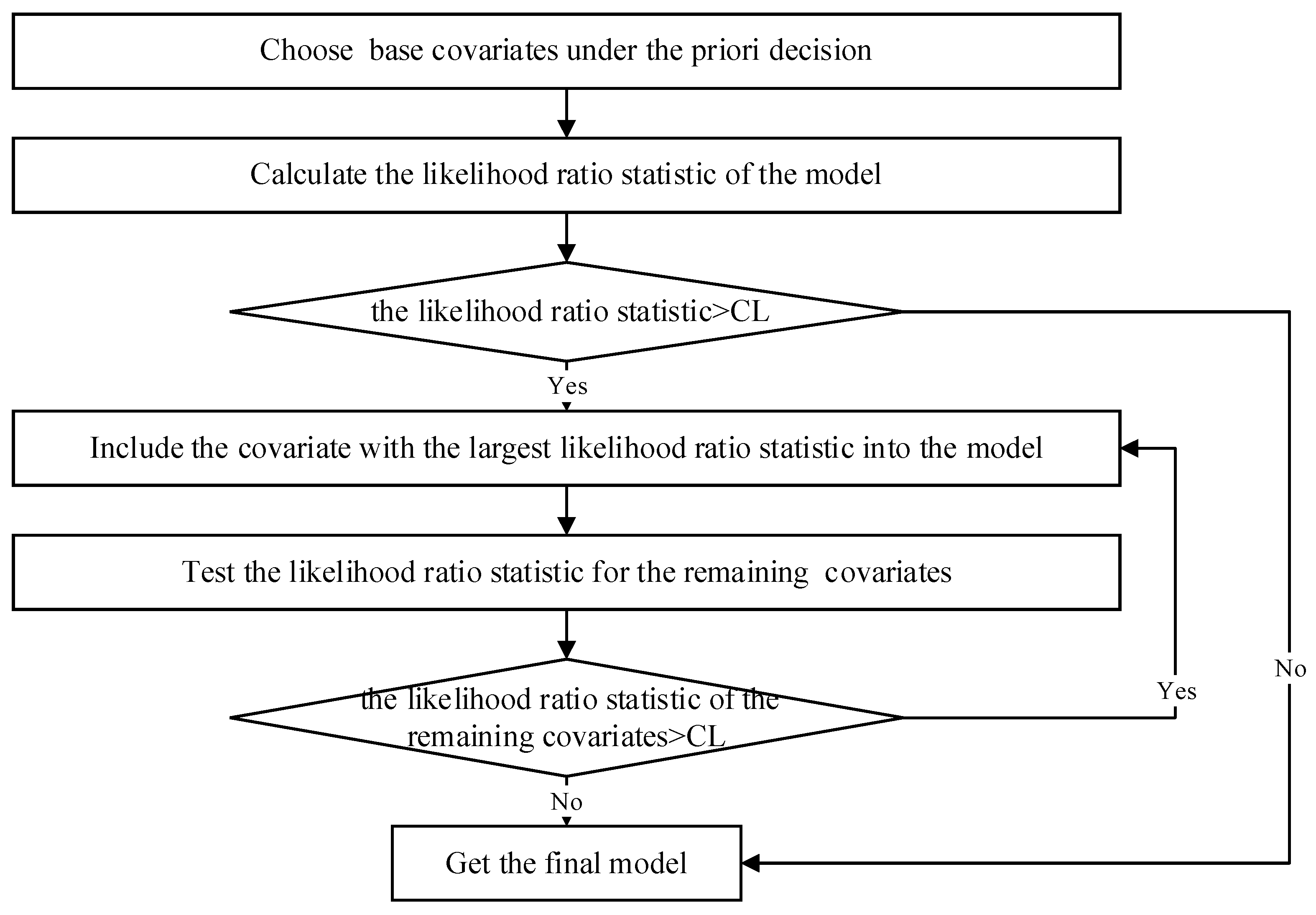
2.1.3. Covariate Selection
- (1)
- Choose prior covariates
- (2)
- Add linear combination terms
2.1.4. Calculation of PS Value for Individuals
2.1.5. Trimming
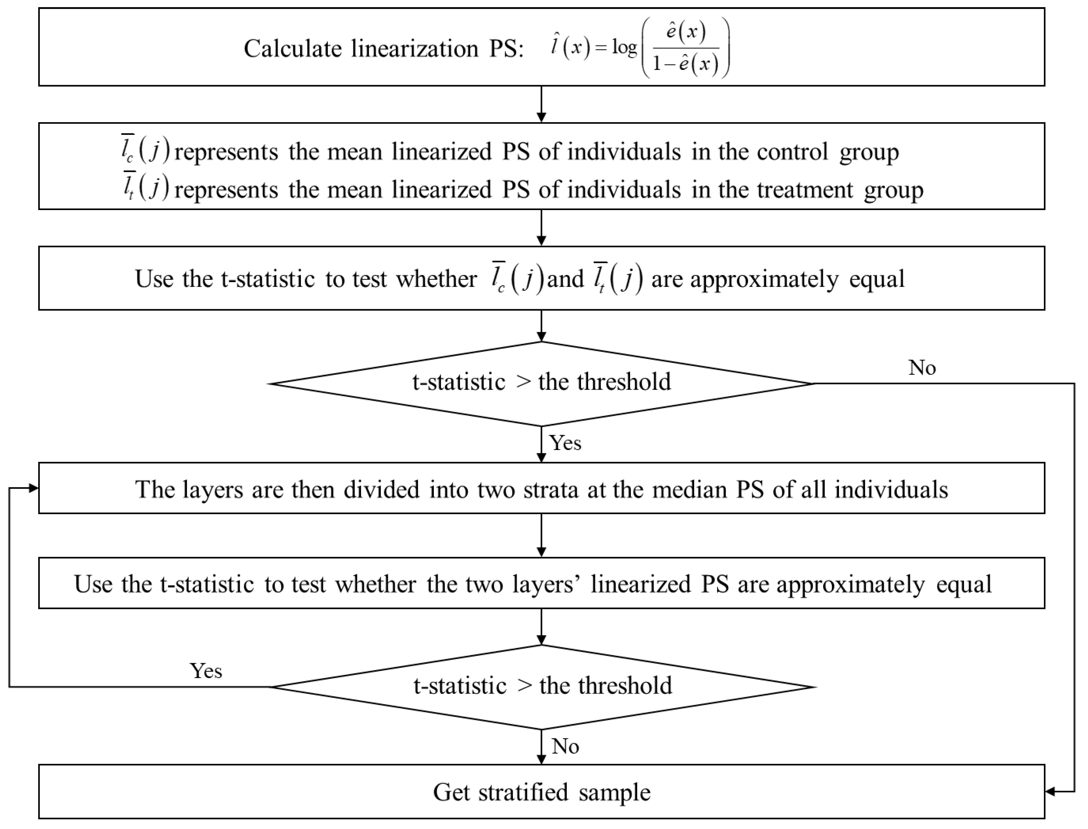
2.2. Stratification
- (1)
- Linearization of PS values
- (2)
- Stratification standard and t-statistic test
- (3)
- The t-statistic is a common measure of the difference of mean values of two groups of data. Considering that the distribution bias in our case study refers to the difference in the mean values between the treatment and control groups, the t-statistic is considered to judge the significance of the difference between treatment and control groups. If the obtained t-statistic exceeds the predefined threshold, it indicates that the PS values in treatment and control groups exhibit a significant difference in this layer and need to be further stratified.
- (4)
- The layers are then further divided into two strata at the median PS of individuals. The two new layers must satisfy the following criterion: the number of control groups and treatment groups in each new layer is not less than , where is the number of covariates. For example, in the process of stratification, if the i-th layer is divided and it is found that the number of samples in treatment/control groups in the new layers is less than , the stratification is stopped even if the t-statistic is not satisfied. This is a stop criterion for the stratification process and the influence is limited as the other stratification process satisfies the t-statistic threshold.
2.3. Calculation of the Average Treatment Effect
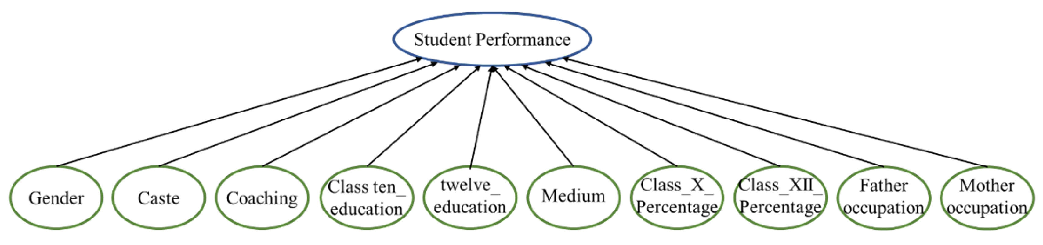
3. Data Description
4. Calculation and Results
4.1. Average Treatment Effect Calculation
4.1.1. Division of Treatment and Control Groups
4.1.2. Select Covariates for Inclusion in Logistic Regression Models
4.1.3. Calculate PS for Sample Data
4.1.4. Trimming
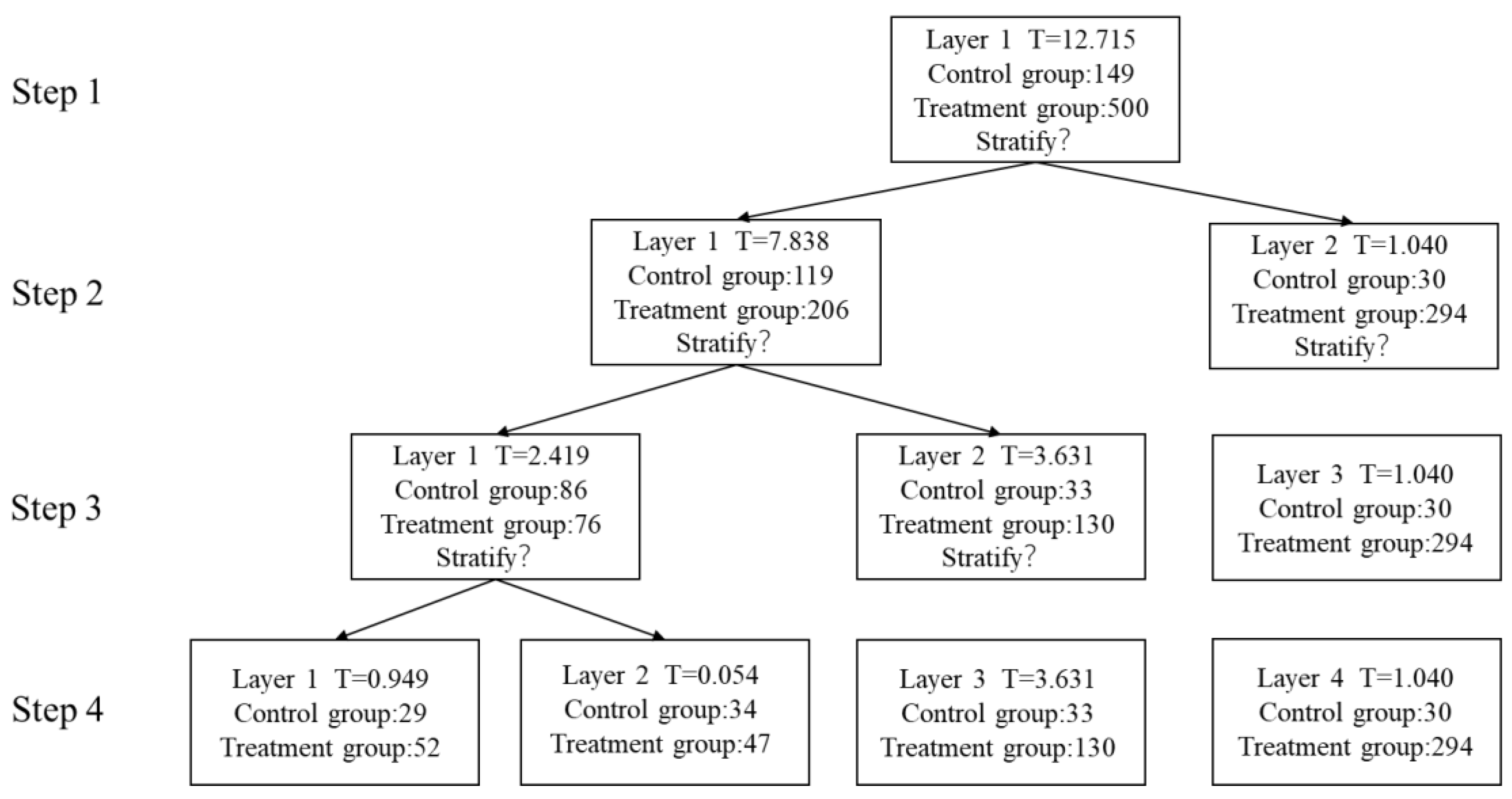
4.1.5. Stratification
- (1)
- The estimated PS is linearized according to Equation (4).
- (2)
- The t-statistic is used to test whether the linear PSs of the treatment and control groups are approximately equal. Before conducting the t-test, the F-statistic is constructed to test whether the variances in the treatment and control groups are comparable. In this case, equal variances are justified with an F-test within each level, so the variances of the two groups are considered equal in the calculation of the t-statistic.
- (3)
- The first stratification
- (4)
- The second stratification
- (5)
- The third stratification
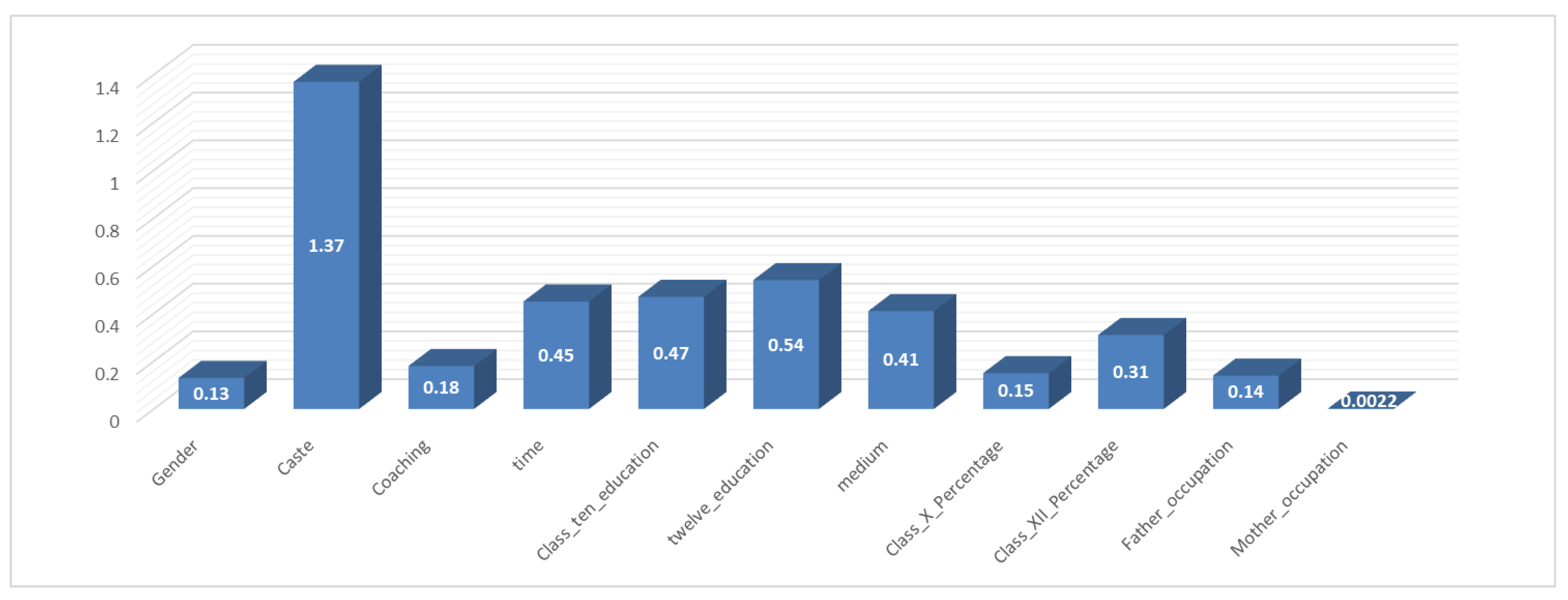
4.1.6. Calculation of Average Treatment Effect
4.2. Average Causal Effect between Response and Other Intervention Variables
4.3. Case Study Result Analysis
- (1)
- The data are obtained from the Dibrugarh University CEE for a given year at a medical school in the Indian state of Assam. In India, caste determines the environment in which individuals are born, the environment and quality of education, as well as other factors. Therefore, the two races ‘SC—Schedule Caste’ and ‘ST—Schedule Tribes’ have lower social status than ‘general’; thus, overall, they have a lower social status in India. There is, not surprisingly, also a large gap in performance on entrance exams based on caste.
- (2)
- Several intervention variables such as time, Class_Ten_education, Twelve_education, and medium are relatively direct influencing factors in the learning process. From the perspective of education, these factors have a certain impact on student performance. This also indicates, however, that students who perform well in Class XII courses also perform well in the entrance examination.
- (3)
- Factors such as parental occupation and gender appear to have little impact on student performance, which indicates that parents’ education level, work environment, and other such factors have little effect on a student’s learning ability or that these factors have an indirect influence rather than a direct one.
- (4)
- To improve student exam performance, the most influential direct factor appears to be caste—that is, social class—but this factor is difficult to change. Therefore, in the field of education, teachers can try to increase the training time of students and choose the appropriate Class_ten_education, Twelve_education, and medium of instruction.
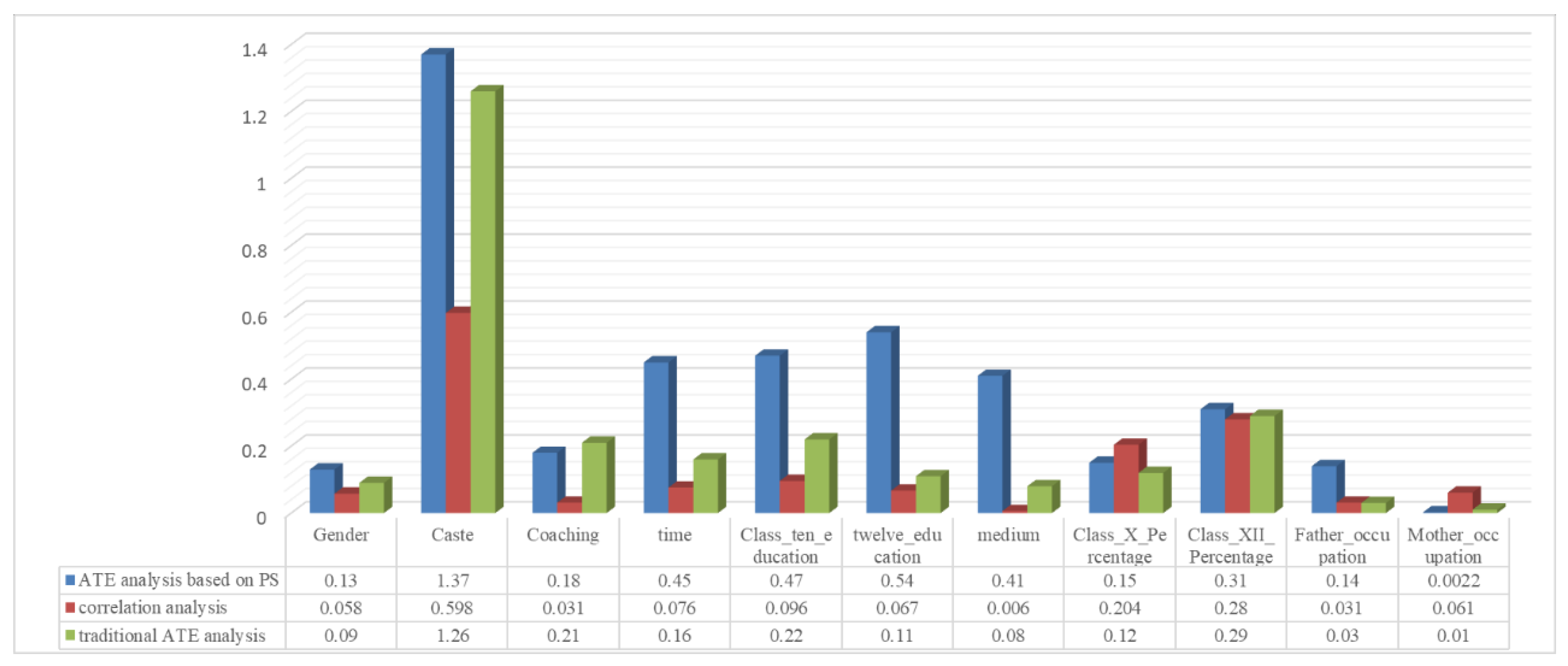
4.4. The Results of Traditional Methods
4.4.1. Correlation Analysis
4.4.2. ATE Calculation Method Based on DoWhy
5. Conclusions
Author Contributions
Funding
Institutional Review Board Statement
Informed Consent Statement
Data Availability Statement
Conflicts of Interest
References
- Clearinghouse, W.W. Standards Handbook; Version 4.0; Institute of Education Sciences: Washington, DC, USA, 2017. [Google Scholar]
- Weiss, M.J.; Bloom, H.S.; Savitz, N.V.; Gupta, H.; Vigil, A.E.; Cullinan, D.N.; Cullinan, D. How Much Do the Effects of Education and Training Programs Vary Across Sites? Evidence From Past Multisite Randomized Trials. J. Res. Educ. Eff. 2017, 10, 843–876. [Google Scholar] [CrossRef]
- Tipton, E.; Olsen, R.B. A Review of Statistical Methods for Generalizing from Evaluations of Educational Interventions. Educ. Res. 2018, 47, 516–524. [Google Scholar] [CrossRef]
- Bosdriesz, J.R.; Stel, V.S.; Van Diepen, M.; Meuleman, Y.; Dekker, F.W.; Zoccali, C.; Jager, K.J. Evidence-based medicine—When observational studies are better than randomized controlled trials. Nephrology 2020, 25, 737–743. [Google Scholar] [CrossRef] [PubMed]
- Wong, V.C.; Valentine, J.; Miller-Bains, K. Empirical Performance of Covariates in Education Observational Studies. J. Res. Educ. Eff. 2017, 10, 207–236. [Google Scholar] [CrossRef]
- Cook, C.; Engelhard, C.; Landry, M.D.; McCallum, C. Modifiable variables in physical therapy education programs associated with first-time and three-year National Physical Therapy Examination pass rates in the United States. J. Educ. Eval. Health Prof. 2015, 12, 44. [Google Scholar] [CrossRef]
- Titus, M.A. Detecting selection bias, using propensity score matching, and estimating treatment effects: An application to the private returns to a master’s degree. Res. High. Educ. 2007, 48, 487–521. [Google Scholar] [CrossRef]
- Chiteng Kot, F. The Impact of Centralized Advising on First-Year Academic Performance and Second-Year Enrollment Behavior. Res. High. Educ. 2014, 55, 527–563. [Google Scholar] [CrossRef]
- Rubin, D.B.; Thomas, N. Characterizing the effect of matching using linear propensity score methods with normal distributions. Biometrika 1992, 79, 797–809. [Google Scholar] [CrossRef]
- Rubin, D.B.; Thomas, N. Matching Using Estimated Propensity Scores: Relating Theory to Practice. Biometrics 1996, 52, 249. [Google Scholar] [CrossRef]
- Lunceford, J.K.; Davidian, M. Stratification and weighting via the propensity score in estimation of causal treatment effects: A comparative study. Stat. Med. 2004, 23, 2937–2960. [Google Scholar] [CrossRef]
- Myers, J.A.; Louis, T.A. Optimal Propensity Score Stratification; Johns Hopkins University, Department of Biostatistics: Baltimore, MD, USA, 2007. [Google Scholar]
- Rosenbaum, P.R.; Rubin, D.B. Reducing bias in observational studies using subclassification on the propensity score. J. Am. Stat. Assoc. 1984, 79, 516–524. [Google Scholar] [CrossRef]
- Hirano, K.; Imbens, G.W. Estimation of Causal Effects using Propensity Score Weighting: An Application to Data on Right Heart Catheterization. Health Serv. Outcomes Res. Methodol. 2001, 2, 259–278. [Google Scholar] [CrossRef]
- Rosenbaum, P.R.; Rubin, D.B. The central role of the propensity score in observational studies for causal effects. Biometrika 1983, 70, 41–55. [Google Scholar] [CrossRef]
- Turk, J.M. Estimating the Impact of Developmental Education on Associate Degree Completion: A Dose–Response Approach. Res. High. Educ. 2019, 60, 1090–1112. [Google Scholar] [CrossRef]
- Vaughan, A.L.; Lalonde, T.L.; Jenkins-Guarnieri, M.A. Assessing Student Achievement in Large-Scale Educational Programs Using Hierarchical Propensity Scores. Res. High. Educ. 2014, 55, 564–580. [Google Scholar] [CrossRef]
- Powell, M.G.; Hull, D.M.; Beaujean, A.A. Propensity Score Matching for Education Data: Worked Examples. J. Exp. Educ. 2020, 88, 145–164. [Google Scholar] [CrossRef]
- Masserini, L.; Bini, M. Does joining social media groups help to reduce students’ dropout within the first university year? Socio-Econ. Plan. Sci. 2021, 73, 100865. [Google Scholar] [CrossRef]
- Chen, J.; Keller, B. Heterogeneous Subgroup Identification in Observational Studies. J. Res. Educ. Eff. 2019, 12, 578–596. [Google Scholar] [CrossRef]
- Suk, Y.; Kang, H.; Kim, J.-S. Random Forests Approach for Causal Inference with Clustered Observational Data. Multivar. Behav. Res. 2021, 56, 829–852. [Google Scholar] [CrossRef]
- Neyman, J.; Iwaszkiewicz, K. Statistical problems in agricultural experimentation. Suppl. J. R. Stat. Soc. 1935, 2, 107–180. [Google Scholar] [CrossRef]
- Rubin, D.B. Estimating causal effects of treatments in randomized and nonrandomized studies. J. Educ. Psychol. 1974, 66, 688–701. [Google Scholar] [CrossRef]
- Holland, P.W. Statistics and causal inference. J. Am. Stat. Assoc. 1986, 81, 945–960. [Google Scholar] [CrossRef]
- Kaplan, D. Causal inference with large-scale assessments in education from a Bayesian perspective: A review and synthesis. Large-Scale Assess. Educ. 2016, 4, 7. [Google Scholar] [CrossRef] [PubMed]
- Morgan, S.L.; Winship, C. Counterfactuals and Causal Inference; Cambridge University Press: Cambridge, MA, USA, 2015. [Google Scholar]
- Yang, S.; Ding, P. Asymptotic inference of causal effects with observational studies trimmed by the estimated propensity scores. Biometrika 2018, 105, 487–493. [Google Scholar] [CrossRef]
- Hussain, S.; Atallah, R.; Kamsin, A.; Hazarika, J. Classification, Clustering and Association Rule Mining in Educational Datasets Using Data Mining Tools: A Case Study. In Proceedings of the Computer Science On-line Conference 2018, Vsetin, Czech Republic, 25–28 April 2018; pp. 196–211. [Google Scholar] [CrossRef]
- Imbens, G.W.; Rubin, D.B. Causal Inference in Statistics, Social, and Biomedical Sciences; Cambridge University Press: Cambridge, MA, USA, 2015. [Google Scholar]
- Neal, B. Introduction to Causal Inference from a Machine Learning Perspective; Course Lecture Notes (Draft). 2020. Available online: https://scholar.google.co.jp/scholar?hl=zh-TW&as_sdt=0%2C5&q=Introduction+to+Causal+Inference+from+a+Machine+Learning+Perspective&btnG=#d=gs_cit&t=1668758477310&u=%2Fscholar%3Fq%3Dinfo%3ATFJuQPUjj00J%3Ascholar.google.com%2F%26output%3Dcite%26scirp%3D0%26hl%3Dzh-TW (accessed on 13 November 2022).
- Sharma, A.; Kiciman, E. DoWhy: An end-to-end library for causal inference. arXiv 2020, arXiv:2011.04216. [Google Scholar]


| Variable | Description | Values |
|---|---|---|
| Performance | Performance in Common Entrance Examination (CEE) | {‘Excellent’, ‘Vg’, ‘Good’, ‘Average’} If the percentage is top 100, Excellent If the percentage is next 200, Very Good (Vg) If the percentage is next 200, Good Remainder, Average Here, the percentage means the percentage score on the CEE Examination |
| Gender | Gender of the candidate | {‘male’, ‘female’} |
| Caste | Caste of the candidate | {‘General’, ‘OBC’, ‘SC’, ‘ST’} OBC—Other Backward Caste SC—Schedule Caste ST—Schedule Tribes |
| Coaching | Whether or not the candidate attended any coaching classes within Assam or outside Assam | {‘NO’, ‘WA’, ‘OA’} No—No Coaching WA—Within Assam OA—Outside Assam |
| Time | The length of time students received coaching | {‘ONE’, ‘TWO’, ‘THREE’, ‘FOUR’, ‘FIVE’, ‘SEVEN’} |
| Class ten_ education | Name of the board where the candidate studied at Class X level | {‘SEBA’, ‘OTHER’, ‘CBSE’} |
| twelve_ education | Name of the board where the candidate studied at Class XII level | {‘AHSEC’, ‘CBSE’, ‘OTHER’} |
| medium | Medium of instruction for the study at the Class XII level | {‘ENGLISH’, ‘OTHER’, ‘ASSAMESE’} |
| Class_X_Percentage | The percentage secured by the candidate at Class X standard | {‘Excellent’, ‘Vg’, ‘Good’, ‘Average’} If the percentage is above 80%, Excellent If 70% ≤ percentage < 80%, Very Good (Vg) If 60% ≤ percentage < 70%, Good The remainder, Average |
| Class_XII_Percentage | The percentage secured by the candidate at Class XII standard | {‘Excellent’, ‘Vg’, ‘Good’, ‘Average’} If the percentage is above 80%, Excellent If 70% ≤ percentage < 80%, Very Good (Vg) If 60% ≤ percentage < 70%, Good The remainder, Average |
| Father occupation | The occupation of the father of the candidate | {‘DOCTOR’, ‘SCHOOL_TEACHER’, ‘BUSINESS’, ‘COLLEGE_TEACHER’, ‘OTHER’, ‘BANK_OFFICIAL’, ‘ENGINEER’, ‘CULTIVATOR’} |
| Mother occupation | The occupation of the mother of the candidate | {‘OTHER’, ‘HOUSE_WIFE’, ‘SCHOOL_ TEACHER’, ‘DOCTOR’, ‘COLLEGE_TEACHER’, ‘BANK_ OFFICIAL’, ‘BUSINESS’, ‘CULTIVATOR’, ‘ENGINEER’} |
| Intervention Variables | Treatment Group | Control Group |
|---|---|---|
| Gender | Male | Female |
| Caste | General, OBC | SC, ST |
| Coaching | WA, OA | NO |
| Time | THREE, FOUR, FIVE, SEVEN | ONE, TWO |
| Class_ten_education | SEBA | Other, CBSE |
| twelve_education | CBSE | AHSEC, Other |
| Medium | English | Other, Assamese |
| Class_X_Percentage | Excellent | Vg, Good, Average |
| Class_XII_Percentage | Excellent | Vg, Good, Average |
| Father’s occupation | SCHOOL_TEACHER, COLLEGE_TEACHER | DOCTOR, BUSINESS, OTHER, BANK_OFFICIAL, ENGINEER, CULTIVATOR |
| Mother’s occupation | HOUSE_WIFE | SCHOOL_TEACHER, DOCTOR, COLLEGE_TEACHER, BANK_OFFICIAL, BUSINESS, CULTIVATOR, ENGINEER, OTHER |
| Covariate | Step | |||||||||
|---|---|---|---|---|---|---|---|---|---|---|
| 1 | 2 | 3 | 4 | 5 | 6 | 7 | 8 | 9 | 10 | |
| Gender | 5.012 | 3.923 | 5.926 | 5.935 | 6.070 | 7.593 | 7.173 | 5.831 | 5.729 | 6.317 |
| Caste | 474.493 | |||||||||
| Time | 21.36 | 18.071 | 16.781 | 18.541 | 26.074 | |||||
| Class_ten_education | 12.164 | 11.521 | 7.322 | 7.542 | 6.564 | 7.592 | 7.048 | 16.441 | ||
| twelve_education | 8.894 | 6.437 | 4.298 | 4.468 | 4.216 | 7.319 | 8.962 | |||
| Medium | 31.220 | 20.703 | 20.075 | 19.472 | 18.338 | 18.760 | ||||
| Class_X_Percentage | 40.910 | 11.458 | 11.762 | 11.950 | 6.355 | 2.943 | 3.067 | 3.703 | 15.242 | |
| Class_XII_Percentage | 72.628 | 24.394 | 21.414 | 21.854 | ||||||
| Father’s occupation | 64.999 | 38.281 | ||||||||
| Mother’s occupation | 46.597 | 37.237 | 32.471 | |||||||
| Step | Layer | Lower Bound | Upper Bound | Interval Width | Number in Control Group | Number in Treatment Group | t-Statistic |
|---|---|---|---|---|---|---|---|
| 1 | 1 | 0.04 | 0.98 | 0.94 | 149 | 500 | 12.715 |
| Step | Layer | Lower Bound | Upper Bound | Interval Width | Number in Control Group | Number in Treatment Group | t-Statistic |
|---|---|---|---|---|---|---|---|
| 2 | 1 | 0.04 | 0.86 | 0.82 | 119 | 206 | 7.838 |
| 2 | 2 | 0.86 | 0.98 | 0.12 | 30 | 294 | 1.040 |
| Step | Layer | Lower Bound | Upper Bound | Interval Width | Number in Control Group | Number in Treatment Group | t-Statistic |
|---|---|---|---|---|---|---|---|
| 3 | 1 | 0.04 | 0.59 | 0.55 | 86 | 76 | 2.419 |
| 3 | 2 | 0.59 | 0.86 | 0.27 | 33 | 130 | 3.631 |
| 3 | 3 | 0.86 | 0.98 | 0.12 | 30 | 294 | 1.040 |
| Step | Layer | Lower Bound | Upper Bound | Interval Width | Number in Control Group | Number in Treatment Group | t-Statistic |
|---|---|---|---|---|---|---|---|
| 4 | 1 | 0.04 | 0.49 | 0.45 | 29 | 52 | 0.949 |
| 4 | 2 | 0.49 | 0.59 | 0.1 | 34 | 47 | 0.054 |
| 4 | 3 | 0.59 | 0.86 | 0.27 | 33 | 130 | 3.631 |
| 4 | 4 | 0.86 | 0.98 | 0.12 | 30 | 294 | 1.040 |
| Layer | 1 | 2 | 3 | 4 |
|---|---|---|---|---|
| Value | −0.21 | 0.27 | 0.45 | −0.6 |
| Intervention Variables | ATE Value |
|---|---|
| Gender | −0.13 |
| Caste | −1.37 |
| Coaching | −0.18 |
| time | 0.45 |
| Class_ten_education | −0.47 |
| twelve_education | −0.54 |
| medium | 0.41 |
| Class_X_Percentage | 0.15 |
| Class_XII_Percentage | 0.31 |
| Father_occupation | 0.14 |
| Mother_occupation | 0.0022 |
| Intervention Variables | Correlation Value |
|---|---|
| Gender | 0.058 |
| Caste | 0.598 ** |
| Coaching | 0.031 |
| time | −0.076 * |
| Class_ten_education | −0.096 * |
| twelve_education | 0.067 |
| medium | −0.006 |
| Class_X_Percentage | 0.204 ** |
| Class_XII_Percentage | 0.280 ** |
| Father_occupation | 0.031 |
| Mother_occupation | −0.061 |
| Intervention Variables | ATE Value |
|---|---|
| Gender | 0.09 |
| Caste | 1.26 |
| Coaching | 0.21 |
| time | −0.16 |
| Class_ten_education | −0.22 |
| twelve_education | −0.11 |
| medium | −0.08 |
| Class_X_Percentage | −0.12 |
| Class_XII_Percentage | 0.29 |
| Father_occupation | 0.03 |
| Mother_occupation | −0.01 |
Publisher’s Note: MDPI stays neutral with regard to jurisdictional claims in published maps and institutional affiliations. |
© 2022 by the authors. Licensee MDPI, Basel, Switzerland. This article is an open access article distributed under the terms and conditions of the Creative Commons Attribution (CC BY) license (https://creativecommons.org/licenses/by/4.0/).
Share and Cite
Liang, J.; Liu, J. Evaluation of Educational Interventions Based on Average Treatment Effect: A Case Study. Mathematics 2022, 10, 4333. https://doi.org/10.3390/math10224333
Liang J, Liu J. Evaluation of Educational Interventions Based on Average Treatment Effect: A Case Study. Mathematics. 2022; 10(22):4333. https://doi.org/10.3390/math10224333
Chicago/Turabian StyleLiang, Jingyu, and Jie Liu. 2022. "Evaluation of Educational Interventions Based on Average Treatment Effect: A Case Study" Mathematics 10, no. 22: 4333. https://doi.org/10.3390/math10224333
APA StyleLiang, J., & Liu, J. (2022). Evaluation of Educational Interventions Based on Average Treatment Effect: A Case Study. Mathematics, 10(22), 4333. https://doi.org/10.3390/math10224333