A Method Combining Multi-Feature Fusion and Optimized Deep Belief Network for EMG-Based Human Gait Classification

Abstract

In this paper, a gait classification method based on the deep belief network (DBN) optimized by the sparrow search algorithm (SSA) is proposed. The multiple features obtained based on surface electromyography (sEMG) are fused. These functions are used to train the model. First, the sample features, such as the time domain and frequency domain features of the denoised sEMG are extracted and then the fused features are obtained by feature combination. Second, the SSA is utilized to optimize the architecture of DBN and its weight parameters. Finally, the optimized DBN classifier is trained and used for gait recognition. The classification results are obtained by varying different factors and the recognition rate is compared with the previous classification algorithms. The results show that the recognition rate of SSA-DBN is higher than other classifiers, and the recognition accuracy is improved by about 2% compared with the unoptimized DBN. This indicates that for the application in gait recognition, SSA can optimize the network performance of DBN, thus improving the classification accuracy.

1. Introduction

Gait is a biological characteristic that describes the manner in which people walk [1]. Walking is one of the important activities that maintains our daily life [2] and physical health. Surface electromyography (sEMG) is a weak bioelectric signal that characterizes to some extent the functional state between the human nervous system and muscles [3]. By analyzing the characteristics of surface electromyography signals obtained from the lower limbs of humans, we can identify the gait phase of the gait cycle [4]. Gait classification based on sEMG signals has been widely used in the diagnosis of muscle diseases and as a guidance path for rehabilitation medicine [5].

Gait information includes video image, electromyography, three-dimensional and kinematics [6,7,8], etc. The 3D motion capture is an accurate optical motion capture system, which can collect and record the 3D gait of the human body in real time and conduct quantitative analysis on gait indicators such as time distance parameters and kinematic parameters. It is commonly used in motion capture and analysis of high frequency and high-precision motion [9,10,11]. The sEMG signal can reflect the activation degree of skeletal muscle and is highly correlated with muscle force [12]. Therefore, sEMG has been widely utilized in the field of gait analysis [13,14]. The gait changes caused by diseases have also attracted extensive attention, accompanied by neuromuscular changes [15,16,17]. With the development of the real-time monitoring system, much research has been conducted to distinguish gait differences between patients and healthy people, and gait indicators can now be effectively evaluated [18,19,20].

The acquired sEMG signals require preprocessing, such as noise elimination and feature extraction before they can be used for performing classification. The process of feature extraction directly affects the final classification performance of gait classification. Depending on the differences between the extracted features, they can be classified into time domain (TD), frequency domain (FD), time-frequency domain, and nonlinear features [21]. The TD features are extracted directly from the original sEMG time series signals without applying any transformation. As a result, the process for extracting these features is easy to implement and has low computational requirements [22]. However, as sEMG signals are susceptible to interference caused due to physical fatigue and other factors, the TD features tend to suffer from severe abrupt changes and poor stability [23]. The FD feature denotes the Fourier transform of the signal. It accurately characterizes the spectrum information of the signal. It is now customary to transform the signal from the time domain to the frequency domain for performing signal analysis [24]. However, the TD and FD features have poor effects on some data types. Hu et al. [25] observed that the traditional time or frequency domain analysis methods are unable to meet the requirements of mechanical faults and several dimensionless coefficients in high dimensional feature sets that reduce the accuracy and the fault identification speed of the diagnostic system. In order to address this phenomenon, Phinyomark et al. [23] used the TD and FD features to classify the upper limb movements by using the recorded EMG data and observed that the combination of these features improved the classification performance as compared to using single domain features. Sejdic et al. [26] used gait accelerometers to extract gait features of the elderly in time domain, frequency domain, and time-frequency domain respectively. The results showed that different feature sets could better distinguish between healthy people and patients with Parkinson’s disease and extract more differences in features between different groups.

Recently, the requirements for the classification accuracy of sEMG signals have increased [27,28]. Common myoelectric signal classification methods include the support vector machine (SVM) [29], linear discriminant analysis (LDA) [30], and the extreme learning machine (ELM) [31,32,33,34,35]. Vikas et al. [36] used SVM with LDA for extracting the TD features from sEMG to build a gesture classification model and combined it with optimization algorithms, such as particle swarm (PSO) and ant colony (ACO) to improve accuracy. Zhao et al. [37] combined ELM with gas chromatography-mass spectrometry (GC-MS) to diagnose paraquat poisoning, and compared it with six methods. The authors observed that ELM effectively distinguished the poisoned patients. Although a variety of methods that combine optimization algorithms with classification algorithms for improving the classification have been presented in the literature [13], research also shows that the traditional SVM easily falls into the local optima, resulting in poor classification results. In addition, ELM is prone to over fitting. Moreover, the traditional algorithms rely on the extraction of TD and FD features [38], and the instability of TD features often leads to a decrease in the final classification accuracy.

In gait classification, the differences between the stride length, walking speed, and the fatigue of the lower limb muscles [14] can lead to significant differences in the distribution of single features extracted from the time or frequency domains [39,40]. The deep belief network (DBN), i.e., a typical representative deep learning architecture can discover the distributed features based on the low-dimensional features for constructing a more abstract high-dimensional representation [41]. This model learns layer by layer based on the low-dimensional signals by using greedy learning and automatically obtains the high-dimensional features. This not only enables us to avoid the complexity and uncertainty caused due to the traditional feature engineering, but also improves the generalization ability of the algorithm [42,43]. Qiu et al. [44] used DBN to forecast the intrinsic modular functions in electricity load demand and to model each function to predict its trend. The final forecasts were derived from a combination of unbiased and weighted summation. Mohammad et al. [45] used DBN to extract the depth features from the fusion observation of signals for classifying five basic emotions. As compared with traditional SVM, DBN significantly improved the accuracy of emotion classification and increased the nonlinear classification of emotions. Qiao et al. [46] combined cognitive computing, DBN, and collaborative robots for building a model. The experiment shows that DBN significantly reduced the error rate by using its own neuron number, network structure, and training epochs and laid a foundation for the performance improvement of collaborative robots for the future. However, the self-parameters of these DBNs which are often determined by human experience, not only induce human diagnostic errors, but also affect the structure of the network. This leads to high computational cost and slow training speed of the whole model [47]. Deng et al. [48] proposed a differential evolution algorithm based on quantum computation to optimize DBN and applied it to the practical engineering problems. The results show that this algorithm has better optimization performance and classification accuracy as compared to non-optimized DBN. Xu et al. [49] proposed the sparrow search algorithm (SSA), which improves the convergence speed, stability, and convergence accuracy of the model. Li et al. [50] used simulated annealing (SA), PSO, and SSA to develop an improved DBN model by selecting the best model parameters. The results show that SSA-DBN achieves the highest assessment accuracy and is suitable for optimizing the network structure of DBN.

In this study, the TD and FD features are extracted from the sEMG signals, and their fusion features are used as the input of a DBN model for performing gait classification. The SSA with better optimization performance is used to adjust the network architecture of DBN and solve the problem of the empirical selection of DBN parameters.

The major contributions of this work are as follows:

(1)

The layer-by-layer learning feature of DBN can solve the distribution differences of feature sets caused by gait differences.

(2)

To solve the problem of empirical selection of DBN parameters, SSA with good optimization performance is used to prevent the model from falling into local optimization due to traditional low dimensional features in gait analysis.

(3)

The proposed method effectively improves the accuracy of gait classification.

The rest of the manuscript is organized as follows. Section 2 describes the proposed methods. Section 3 presents the experimental results and discussion. Section 4 concludes this work and presents the future work.

2. Materials and Methods

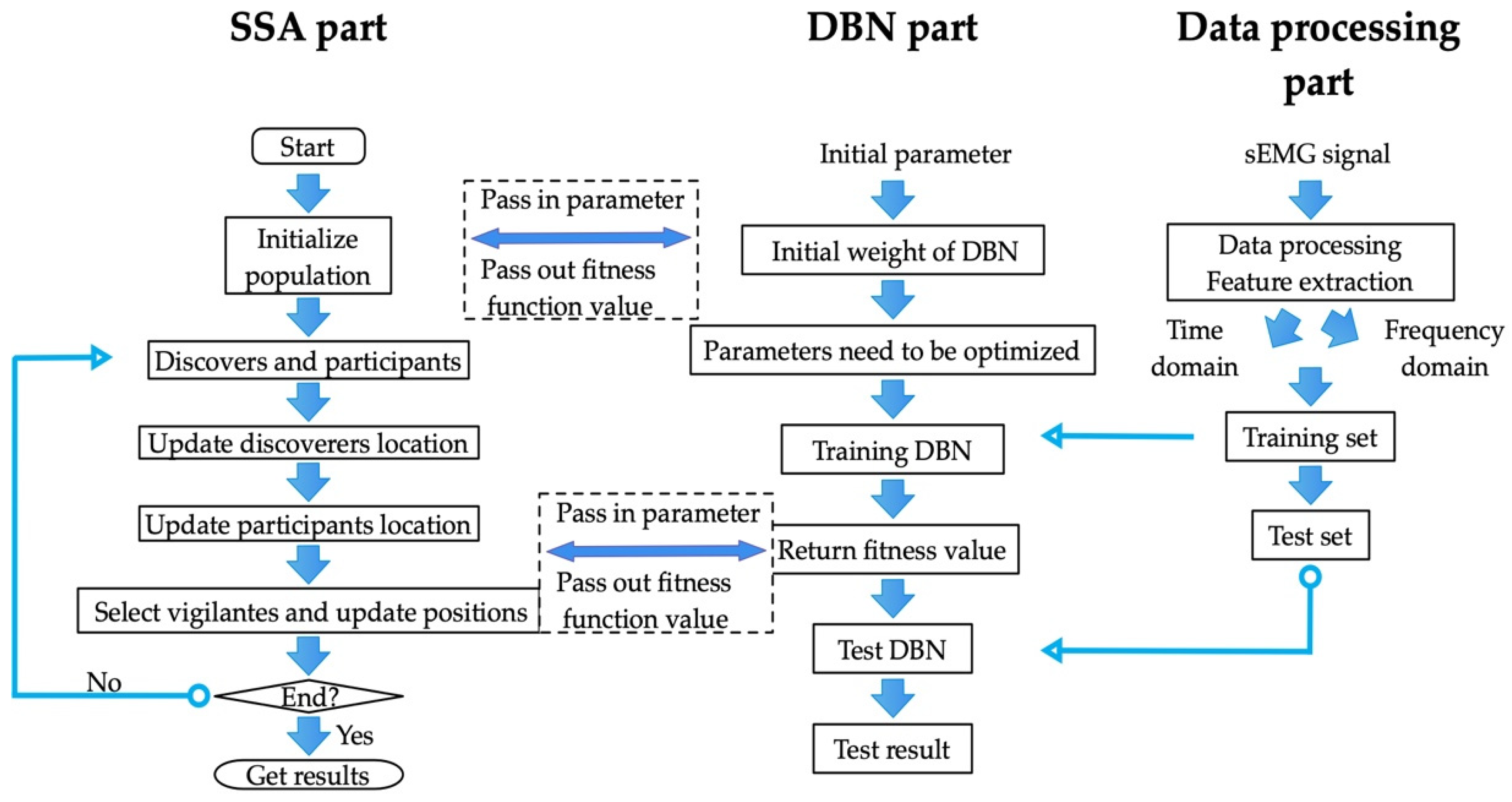
This experimental protocol is comprised of five parts, namely acquisition of experimental data and its pre-processing, feature extraction from sEMG signals, construction of the deep belief network (DBN), parameter optimization of SSA, and gait classification results. The flowchart of the proposed method is shown in Figure 1.

2.1. Lower Limb Muscle Selection and sEMG Signals Processing

2.1.1. Lower Limb Muscles and Gait Division

Considering the role and contribution of lower limb muscles during different phases of walking, and the sensitivity of the sEMG signal acquisition device to lower limb muscles, the muscles with distinct performance characteristics are selected as the signal sources [51]. As presented in Figure 2, it includes tensor fascia lata (TF), adductor longus (AL), rectus femoris (RF), vastus medialis (VM), tibialis anterior (TA), semitendinosus (ST), gastrocnemius (GM), and soleus (SO).

A complete gait cycle can be divided into stance and swing phases [52]. The stance phase can be further divided into pre-stance, mid-stance, and terminal-stance. The swing phase can be divided into pre-swing and terminal-swing, as presented in Figure 3.

2.1.2. Signal Processing and Analysis

The surface electromyography (sEMG) signal is a complex, weak, and non-smooth electrical signal, which comprises motion artifacts caused by electrode offset and other noise interference induced during the acquisition process. Therefore, it is necessary to remove the noise efficiently. The denoising methods we adopted in the experiment include wavelet threshold denoising, wavelet packet threshold denoising, and wavelet modulus maximum denoising [53].

2.2. Feature Extraction of sEMG Signals

After de-noising, the TD and FD features of each channel of the EMG signal are extracted. In this work, three representative time domain characteristics, including absolute mean value (MAV), variance (VAR), and zero crossing points (ZC) are used as frequency domain features [54,55].

MAV takes advantage of the property that sEMG signals have large amplitude fluctuations in the time domain, which are linearly related to the level of muscle activation. The higher the value of MAV, the higher is the activation level of the muscle.

$$\mathrm{MAV}=\frac{1}{N}{\displaystyle \sum _{k=1}^N\left|x_k\right|}$$

(1)

where, $x_k\left(k=1,2,\dots ,N\right)$ denotes the sEMG time series with a window length of N.

VAR is a measure of signal power of the sEMG signal and is expressed as follows:

$$\mathrm{VAR}=\frac{1}{N-1}{\displaystyle \sum _{k=1}^N{x}_k^2}$$

(2)

ZC refers to the number of times that the sEMG waveform passes through the zero point to avoid signal cross counting caused by low-level noise. It is mathematically expressed as follows:

$$\mathrm{ZC}={\displaystyle \sum _{k=1}^N\mathrm{sgn}\left(-x_k{x}_{k+1}\right)}$$

(3)

where, $\mathrm{sgn}(x)=\left\{\begin{array}{cc}1& x>0\\ 0& \mathrm{otherwise}\end{array}\right.$.

We select two representative frequency domain characteristics, namely average power frequency $f_{mean}$ and median frequency $f_{mf}$ [56] defined as follows:

$$f_{mean}=\frac{{\displaystyle {\int }_0^{+\infty }fP\left(f\right)df}}{{\displaystyle {\int }_0^{+\infty }P\left(f\right)df}}$$

(4)

$${\displaystyle {\int }_0^{f_{mf}}P(f)df=}{\displaystyle {\int }_{f_{mf}}^{+\infty }P(f)df=\frac{1}{2}{\displaystyle {\int }_0^{+\infty }P(f)df}}$$

(5)

where, $P\left(f\right)$ is the power spectral density of the sEMG signal and $f$ is the frequency.

Each feature is extracted by setting different window lengths N and to form a set of feature vectors. Then, a set of feature matrices is formed based on different kinds of selected lower limb muscles, where the number of rows in the matrix represents the number of selected lower limb muscle blocks and the number of columns represents the values of the windows in which the signal is divided. This feature matrix is used as the input data of the network in the next section.

2.3. Deep Belief Network

The deep belief network (DBN) is a probabilistic generation model that is designed by stacking multiple restricted Boltzmann machines (RBMs). Its training process is divided into two parts, i.e., the greedy unsupervised hierarchical pre-training process and the discriminative supervised fine-tuning process. Please note that the neurons in the same layer are not connected to each other and connections are only formed between adjacent layers [57].

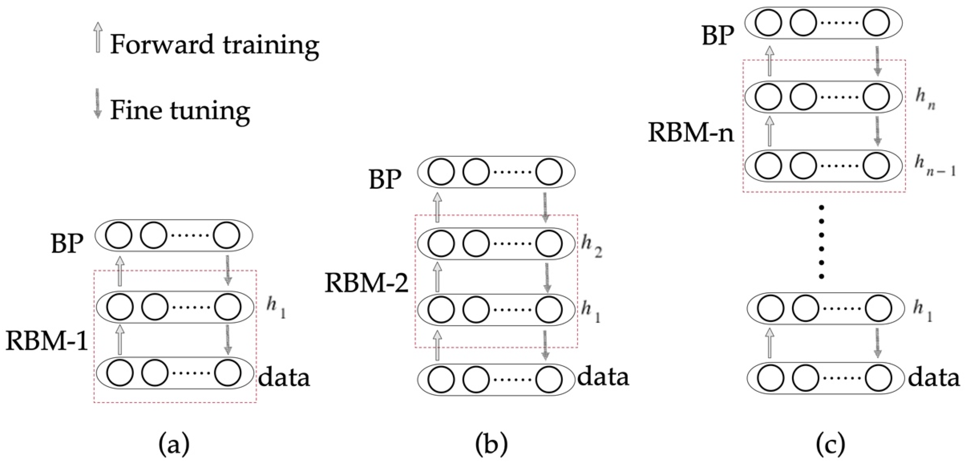
The basic building module of DBN is RBM. One RBM is composed of one visible layer and one hidden layer. During the training process of DBN, each RBM is usually pretrained from bottom to top in a layered manner, and the hidden layer of the previous RBM is used as the visible layer of the next RBM. Afterwards, the whole DBN model is fine-tuned based on the BP network set in the last layer. Finally, the output layer performs hypothesis prediction according to the posterior probability distribution obtained in the previous layer.

The basic network structure of the DBN model is shown in Figure 4. In this work, we define the learning rate factor controlling the weight update rate as $\alpha$ and the number of fine-tunings as $\beta$.

Figure 4a–c represents the structure of the DBN model containing 1 RBM, 2 RBMs, and n RBMs, respectively. The first RBM is composed of the feature matrix data obtained in the previous section and the first hidden layer $h_1$. The parameters of the first RBM are trainable, and include the weights and offset coefficients of $h_1$. Then, $h_1$ is treated as the visible vector and $h_2$ as the hidden vector, and the second RBM is trained. The third RBM is trained in a similar fashion. The black circles in Figure 4 represent the neurons of each layer. The number of neurons is usually determined manually. In this work, the number of neurons is set as Best_pos ($q$) (where $q$ represents the $q$-th hidden layer and $q\in \left[1,n\right]$).

The architecture of DBN possesses the ability to obtain higher dimensional features based on the layer-by-layer learning feature of this model. The hidden variables in each layer learn how to represent the high-order correlations of the original input data. In order to use DBN for classification, the feature vectors of the data samples are used to set the state of the visible variables in the bottom layer of DBN. This is followed by DBN generating a probability distribution of the possible labels of the data based on the posterior probability distribution of the data samples.

Let us assume that the dataset $S=\left\{\left(c_1,d_1\right),\left(c_2,d_2\right),\dots ,\left(c_M,d_M\right)\right\}$ contains $M$ data sample pairs, where $c_M$ is the $M$-th data sample and $d_M$ is the corresponding $M$-th target tag. Given a data sample $\left(c_{\lambda },d_{\lambda }\right)$ ($\lambda \in \left[1,M\right]$) from the data set, the DBN with $n$ hidden layers is represented as a complex feature mapping function. After feature conversion, the softmax layer is used as the output layer of the DBN to classify and predict the parameter ${\theta }_{\lambda }=\left\{{\omega }_{\lambda }+h_{\lambda }\right\}$. If there are $K$ neurons in the softmax layer, then the $o$-th ($o\in \left[1,K\right]$) neuron is responsible for predicting the probability of the $o$-th class. The input of a given $c_n$ is the output of the previous layer and is associated with the weight $W_{\lambda }^{\left(o\right)}$ and the offset $b_{\lambda }^{\left(o\right)}$. The probability obtained by the softmax layer is mathematically expressed as follows:

$$P\left(d=o|c\right)=\frac{\exp \left(b_{\lambda }^{\left(o\right)}+c_n^T{W}_{\lambda }^{\left(o\right)}\right)}{{\displaystyle \sum _{k=1}^K\exp \left(b_{\lambda }^{\left(k\right)}+c_n^T{W}_{\lambda }^{\left(k\right)}\right)}}$$

(6)

where, $c_n$ denotes the output of the previous layer. Based on probability estimation, the trained DBN classifier provides the following prediction.

$$f(c)=\arg \underset{1\le o\le K}{\max }P\left(d=o|c\right)$$

(7)

The DBN is optimized by the statistical gradient descent with negative log-likelihood loss relative to the training set $S$. The posterior of each layer is approximated by the factorial distribution of independent variables within a layer. The values of the independent variables are provided by the variables in the previous layer. The purpose of the wake-sleep algorithm [57] is to learn the characteristics of the original data and recover it correctly. It obtains the weights of the top-level undirected connections by fitting RBM on the posterior distribution of the penultimate layer. The fine-tuning process starts with the state of the top output layer and in turn activates each bottom layer by using a top-down connection. Thus, a DBN model can be considered as RBMs consisting of all prior hidden variables placed at the top layer of a directed belief network, combined with a set of “identified” weights to perform fast approximate inference.

2.4. Sparrow Search Algorithm

The sparrow search algorithm (SSA) is a metaheuristic algorithm that is inspired by the characteristics of birds, i.e., foraging and anti-predatory behavior [49].

Let us suppose that a population of $w$ sparrows conducts a search for food.

$$E=\left[\begin{array}{cccc}{e}_1^1& e_1^2& \cdots & e_1^v\\ e_2^1& e_2^2& \cdots & e_2^v\\ \cdots & \cdots & e_i^j& \cdots \\ e_w^1& e_w^2& \cdots & e_w^v\end{array}\right]$$

(8)

where, $v$ denotes the dimension of the problem variable to be optimized and $w$ represents the number of sparrows, and $i\in \left[1,w\right]$, $j\in \left[1,v\right]$. At this point, the fitness value is expressed as follows:

$$R_e=\left[\begin{array}{c}r\left(\left|\begin{array}{cccc}{e}_1^1& e_1^2& \cdots & e_1^v\end{array}\right|\right)\\ r\left(\left|\begin{array}{cccc}{e}_2^1& e_2^2& \cdots & e_2^v\end{array}\right|\right)\\ \cdots \\ r\left(\left|\begin{array}{cccc}{e}_w^1& e_w^2& \cdots & e_w^v\end{array}\right|\right)\end{array}\right]$$

(9)

where, $r$ denotes the fitness value.

The sparrows with high fitness value have a larger foraging search range as discoverers as compared to the joiners in the population. Therefore, the location update of the discoverers during each iteration is described as follows:

$$E_{i,j}^{t+1}=\left\{\begin{array}{c}{E}_{i,j}^t\cdot \exp \left(\frac{-i}{\alpha \cdot ite{r}_{\max }}\right),W_2<ST\\ E_{i,j}^t+Q\cdot L,W_2\ge ST\end{array}\right.$$

(10)

where, $t$ is the current iteration, $ite{r}_{\max }$ is the maximum number of iterations, $\alpha$ is a uniformly distributed random number in range $\left[0,1\right]$. $W_2\in \left[0,1\right]$ and $ST\in \left[0.5,1\right]$ denote the warning value and the safety value, respectively. $Q$ is a random number subject to normal distribution, and $L$ is a matrix of dimension $1\times d$. When $W_2<ST$, there is no danger around the population and the discoverer can expand the search range to make the fitness value of other individuals higher. On the other hand, when $W_2\ge ST$, a predator is detected around the population and an alarm is released. As a result, all the sparrows quickly fly to other safe places for feeding.

The update of the joiner’s position during each iteration is described as follows,

$$E_{i,j}^{t+1}=\left\{\begin{array}{c}Q\cdot \exp \left(\frac{E_{worst}^t-E_{i,j}^t}{i^2}\right),i>\frac{n}{2}\\ E_{pbest}^{t+1}+\left|E_{i,j}^t-E_{pbest}^{t+1}\right|\cdot A^{+}\cdot L,\mathrm{otherwise}\end{array}\right.$$

(11)

where, $E_{worst}^t$ and $E_{pbest}^t$ denote the worst global position and the best local position of the joiner in the t-th and (t+1)-th iterations, respectively. $A$ is a multidimensional matrix with internal elements of 1 or −1, and $A^{+}=A^T{\left(A{A}^T\right)}^{-1}$. When $i>\frac{n}{2}$, the $i$-th joiner with lower adaptation has no gain in foraging and should shift its location to obtain higher energy.

The update regarding the position of the population after it becomes aware of the danger is described as follows:

$$E_{i,j}^{t+1}=\left\{\begin{array}{c}{E}_{gbest}^t+\beta \cdot \left|E_{i,j}^t-E_{gbest}^t\right|,r_i>r_g\\ E_{i,j}^t+\mu \cdot \left(\frac{\left|E_{i,j}^t-E_{worst}^t\right|}{\left(r_i-r_{\omega }\right)+\epsilon }\right),r_i=r_g\end{array}\right.$$

(12)

where, $E_{gbest}^t$ is the global optimal position of the current population, $\beta$ is the step control parameter, which is a random number distributed normally with mean 0 and variance 1, and $\epsilon$ is a very small constant used to avoid zero in the denominator. $\mu \in \left[-1,1\right]$ is a random number, $r_i$ is the fitness value of individual $i$, $r_g$, and $r_{\omega }$ are the optimal and the worst fitness values of the current population, respectively. When $r_i>r_g$, it means that the current individual is at the edge of the population and is highly vulnerable to the predators. When $r_i=r_g$, the current individual is in the middle of the population. When it feels the danger, it should move closer to other sparrows to reduce the risk of being predated.

In this work, the SSA is used to search for the sparrow with the best position among the parameters to be optimized in the DBN, i.e., the sparrow with the highest adaptation degree. The parameters include the number of neurons Best_pos ($q$) per layer, the number of reverse fine-tunings $\beta$, and the learning rate $\alpha$ mentioned in the previous section. The optimal network structure of the DBN is set based on the parameters of this sparrow at the end of each iteration.

2.5. Training Process of Gait Results

The detailed steps of the proposed algorithm are presented below.

Step 1. We obtain the original sEMG signals dataset.

Step 2. We denoise the original signal dataset by using the wavelet modulus maximum method.

Step 3. The TD and FD features are extracted by using overlapping windows.

Step 4. The dataset is divided into training and test sets.

Step 5. We set the relevant parameters in the DBN model, including the number of RBM layers, the number of neurons in each layer, the number of iterations, the learning rate, and the number of reverse fine-tunings.

Step 6. We set the parameters of SSA, including the number of optimization parameters, the ratio of discoverers to joiners, and the safety threshold of the optimization parameter value.

Step 7. The DBN randomly generates the initial weights based on the safety threshold. The SSA algorithm updates the positions of the warning values of discoverers and joiners based on (10) and (11), and (12), assigns the updated parameter values to the DBN model, and iteratively updates the values of the new fitness function.

Step 8. We determine whether the termination condition is satisfied and whether the fitness function is the current optimum. If not, return to Step 6, otherwise, proceed to Step 9.

Step 9. Finally, we obtain the minimum value of fitness function value and determine the DBN parameters, i.e., the optimal weight parameters of the DBN model.

Step 10. The trained model is evaluated based on the test set.

The flowchart of the proposed algorithm is presented in Figure 5.

3. Results and Discussion

3.1. Acquisition and Pre-Processing of sEMG Signals from Subjects

The dataset included signals recorded from six healthy adults. Mean (±SD) characteristics were as follows: age = 24.0 ± 1.5 years; height =173 ± 5 cm; mass = 66.3 ± 7.1 kg; body mass index (BMI) = 22.2 ± 1.0 kg/${\mathrm{m}}^2$. None of the subjects presented any pathological condition or had undergone orthopedic surgery that might have affected lower limb mechanics. Therefore, subjects with joint pain, neurological pathology, orthopedic surgery, abnormal gait, or a body mass index (BMI) higher than 25 (overweight and obesity) were not recruited. The research was undertaken in compliance with the ethical principles and participants signed informed consent prior to the beginning of the test. The equipment included a DataLink sEMG acquisition instrument (sampling frequency of 1000 Hz), a Vicon three-dimensional motion capture system, a triaxial accelerometer, and a computer. The subjects walk on a treadmill at a uniform speed of 1.3 m/s for 60 s. The signals from eight muscles, presented in Figure 2, are used as the signal acquisition sources, and synchronous camera tracking is carried out, which is convenient for gait recognition comparison verification. The spatial-temporal information of the subjects’ gait are as follows: the gait cycle is controlled within 1–1.5 s, the step length is 1–1.5 m, and the step speed is 1.3 m/s. Figure 6 shows the 8-channel EMG signal of a complete gait cycle.

The acquired sEMG signals are compared based on three denoising methods, namely, wavelet threshold denoising, wavelet packet threshold denoising, and wavelet modulus maximum denoising. The root mean square error (MSE) and signal to noise ratio (SNR) are used as the evaluation indicators [58]. The following is an example of the vastus medialis (VM) muscle.

Generally, for the two aforementioned evaluation indicators, the smaller the MSE, the larger the SNR, and the better are the noise elimination results. In

Table 1. The SNR and MSE of the three denoising methods.

Index Analysis	Wavelet Modulus Maximum	Wavelet Packet Threshold	Wavelet Threshold
MSE	0.0024	0.0025	0.0034
SNR	92.5751	85.8261	83.0223

, the SNR of the wavelet modulus maximum is greater than the wavelet packet threshold and the wavelet threshold, and the average SNR reaches 92.5751. Similarly, the MSE index of the wavelet modulus maximum method is as low as 0.0024, which is significantly lower than the other two methods. Therefore, in this work, the wavelet modulus maximum method is used to denoise the sEMG signals. The corresponding denoising effect is shown in Figure 7.

Figure 7 represents the denoising result of the selected lower limb muscle. In each subplot, the red curve in the upper panel denotes the original signal before denoising and the blue curve in the lower panel represents the signal after denoising. It is evident from the figure that the original signal contains more burrs and the signal drifts around the zero baseline in the resting state. After using wavelet modulus maximum denoising, the signal curve becomes smoother, and the signal tends to zero in the resting state.

Finally, TD features and FD features are extracted from the denoised signal separately. In this work, the features are extracted using the data window with overlap. The window length N is 30 ms, and each window increment is 25 ms to obtain the pre-processed dataset.

3.2. Classifier Parameter Setting

In this section, SVM, ELM, DBN, and SSA-DBN are used to classify and identify the TD features, FD features, and fusion features obtained by combining TD and FD. The unoptimized DBN model contains 4 layers and 3 RBMs. The number of neurons per layer is 10, the number of epochs is 30, the learning rate is 0.01, and the number of reverse fin e-tunings is set to 10 and 100 to perform comparisons in subsequent experiments.

The SSA algorithm is introduced to optimize the architecture of DBN. In this work, we consider the proportion of discoverers to be 20% and the warning value is 0.8. The SSA algorithm optimizes several parameters. Note that different values of the parameters have certain effects on the classification results. Based on the structure of the network and the size of the dataset, five optimization parameters are set for performing experiments. It is worth noting that the parameters are often determined by human experience from previous studies, so this experiment uses SSA to optimize parameters. The range of the search for obtaining the optimal values is shown in

Table 2. The range of the DBN parameters considered for SSA optimization.

Parameters	Optimization Range
Best_pos (1)	[5, 100]
Best_pos (2)	[5, 100]
Best_pos (3)	[5, 100]
$\alpha$	[0.01, 0.1]
$\beta$	[10, 1000]

.

Where, Best_pos (1), Best_pos (2), and Best_pos (3) are used to limit the number of neurons in the 3 RBMs, $\alpha$ denotes the learning rate, and $\beta$ denotes the number of reverse fine-tunings.

3.3. The Effect of Feature Type on Classification Results

The data sets are obtained from 20 consecutive experiments conducted by six subjects respectively. The classification results in this study are based on statistics, consisting of mean value and standard error [59]. The mean value represents the average recognition rate in the gait phase, and the standard error describes the average difference between the mean recognition rate of different subjects and the mean overall recognition rate. Variance is also an indicator of statistics, which represents the deviation degree between sample and the mean [60]. Finally, the average recognition rate of the five gait results is calculated on the basis of the arithmetic mean.

3.3.1. Time Domain Features

In this section, the DBN and SSA-DBN models use the TD feature dataset of gaits as the input for performing gait classification. The corresponding results are compared with SVM and ELM classifiers. The classification results are shown in

Table 3. The classification results of TD features obtained using various classifiers (%).

Classifier	Pre-Stance	Mid-Stance	Terminal-Stance	Pre-Swing	Terminal-Swing	Average Accuracy
SVM	91.61 ± 1.32	85.31 ± 1.21	91.86 ± 1.32	95.82 ± 1.31	95.78 ± 1.32	92.08
ELM	94.69 ± 1.31	93.16 ± 1.23	94.69 ± 1.14	92.82 ± 1.22	94.38 ± 1.21	93.95
DBN (10)	93.85 ± 1.24	92.29 ± 1.42	93.80 ± 1.21	92.21 ± 1.27	94.72 ± 1.22	93.37
DBN (100)	96.78 ± 1.11	96.51 ± 1.10	95.61 ± 1.12	94.17 ± 1.21	96.78 ± 1.12	95.97
SSA-DBN	97.35 ± 1.13	97.31 ± 1.10	95.28 ± 1.21	94.41 ± 1.22	96.88 ± 1.11	96.24

.

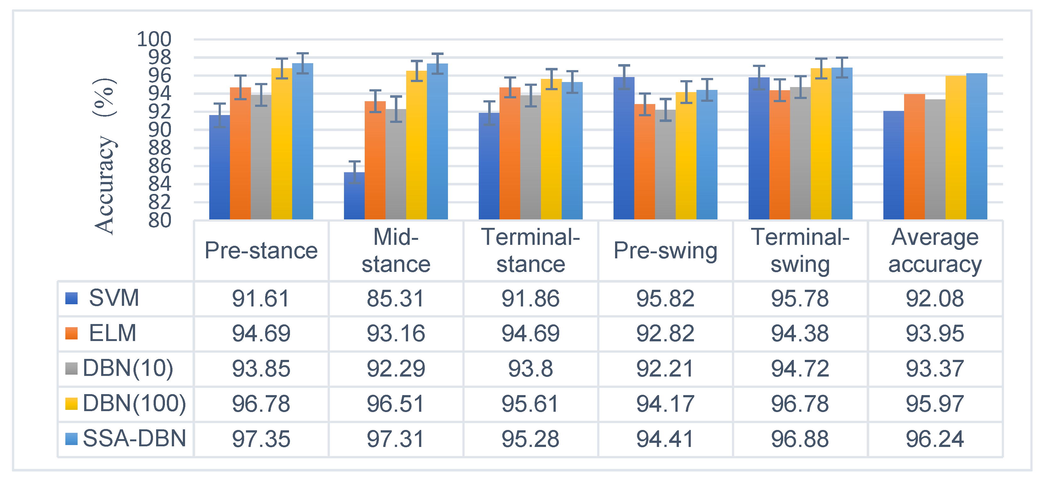
In Table 3, the rows represent the recognition rates trained by the classifier for the five stages of gait classification, i.e., pre-stance, mid-stance, terminal-stance, pre-swing, and terminal-swing. Each column represents different types of classifiers. In order to study the effect of network structure on the DBN model, DBN (10) (the number of reverse fine-tunings of this model is 10) and DBN (100) (the number of reverse fine-tunings of this model is 100) are used. In order to compare the classification results of each classifier more intuitively, a comparison graph is presented in Figure 8.

The analysis of the data presented in Figure 8 shows that the average classification accuracies based on TD features obtained by using SVM, ELM, DBN, and SSA-DBN classifiers are 92.08%, 93.95%, 95.97%, and 96.24%, respectively. The results show that SSA-DBN has the highest average recognition rate and improves the classification accuracy by about 4% compared with SVM. The recognition rate of SVM is significantly lower as compared to classifiers in mid-stance. Based on TD, the classification effect of DBN with reverse fine-tuning number of 10 is not much different from that of the SVM and ELM. Notably, the classification result of DBN with 100 reverse fine-tuning times is significantly better than that of DBN with 10 reverse fine-tuning times. This shows that the training efficiency and classification results can be improved by artificially adjusting the network structure of the DBN model. Therefore, in order to address this situation, we develop a discussion regarding the effect of the number of reverse fine-tunings on the classification results of the TD features.

3.3.2. The Effect of the Number of Reverse Fine-Tunings on TD Feature Classification Results

In this section, the TD features under the pre-stance are considered. First, we set the unoptimized DBN model with 4 layers, 3 RBMs, 10 neurons per layer, 30 training epochs, and a learning rate of 0.01. Then, we artificially adjust the number of reverse fine-tunings to 1, 20, 100, and 500. Second, in order to investigate the effect of the SSA algorithm on the network structure of the DBN model, we use the SSA algorithm to adaptively select the DBN model with the number of reverse fine-tunings $\beta$ for performing comparisons. The corresponding results are presented in

Table 4. The effect of the number of reverse fine-tunings on the recognition rate and training time.

Fine-Tuning Times	Accuracy (%)	Time (s)
1	0	6.81
20	91.79 ± 1.54	10.34
100	93.61 ± 1.21	23.75
$\beta$	96.78 ± 1.10	30.65
500	96.17 ± 1.11	79.02

.

As presented in Table 4, the recognition rate of the DBN model increases as the number of reverse fine-tunings is artificially increased. The results demonstrate that the network structure of the DBN model plays a decisive role in the accuracy of the final gait classification. However, at the same time, the increase in the number of reverse fine-tunings also increases the training time. Moreover, this method also relies on subjective judgment of human experience when solving the practical classification problems.

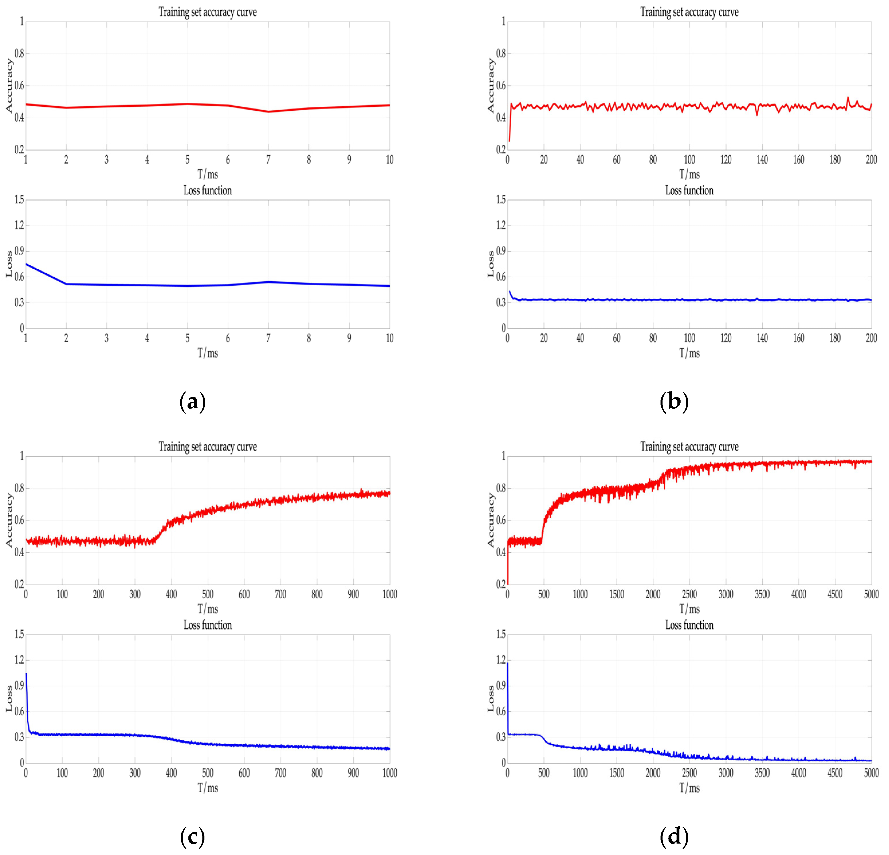
The recognition rate of the model optimized by SSA is the highest. When compared with the DBN with 500 times of reverse fine-tuning, although there is no major improvement in the recognition rate, it greatly reduces the training time, which in turn improves the classification efficiency and avoids human diagnosis errors. On the other hand, it also illustrates the importance of adjusting the network structure to improve the performance of the DBN model. Figure 9 compares the recognition rate curves of the aforementioned models.

We keep the vertical axis range from (a) to (d) in Figure 9 consistent to make the comparison clearer. With the increase of training time, the range of the horizontal axis also increases. It is evident from Figure 9 that when the number of fine-tunings is 1, the curve stability is poor and the recognition rate is extremely low. When the number of fine-tunings is 20, the recognition accuracy is slightly improved, but the curve is still oscillating. After the number of fine-tunings is increased again, the recognition rate curve becomes stable, and the loss function gradually decreases and finally tends to 0. This further illustrates the influence of the network structure on the DBN model. In the subsequent experiments, in order to reduce the invalid workload, reduce the execution time, and facilitate the analysis of the network performance before and after optimization, we fix the number of fine-tunings of the unoptimized DBN model to 100.

3.3.3. Frequency Domain Features

The FD features are used as the input of DBN and SSA-DBN models for performing gait classification and the corresponding results are compared with SVM and ELM classifiers. The classification results are shown in

Table 5. The classification results obtained using FD features with various classifiers (%).

Classifier	Pre-Stance	Mid-Stance	Terminal-Stance	Pre-Swing	Terminal-Swing	Average Accuracy
SVM	94.31 ± 1.32	94.14 ± 1.31	95.03 ± 1.42	95.81 ± 1.10	95.60 ± 1.21	94.97
ELM	94.06 ± 1.41	95.64 ± 1.12	94.69 ± 1.33	95.82 ± 1.11	95.32 ± 1.10	95.10
DBN	96.90 ± 1.10	96.89 ± 1.10	94.31 ± 1.21	96.03 ± 1.12	96.72 ± 1.10	96.17
SSA-DBN	96.81 ± 1.11	97.91 ± 1.00	94.28 ± 1.21	96.51 ± 1.12	96.58 ± 1.12	96.42

.

In Table 5, the rows represent the recognition rates of the classifier for the five stages of gait classification, and each column represents different types of classifiers. Please note that the parameters of the network structure are no longer set artificially for the SSA-DBN model, but the number of reverse fine-tunings is chosen by SSA autonomously from the conclusions drawn in the previous section. In order to compare the classification results of each classifier more intuitively, a comparison graph is presented in Figure 10.

According to the data analysis presented in Figure 10, the average recognition rate of SSA-DBN is the highest, reaching 96.42%, followed by DBN, which is still slightly higher than the other two algorithms. The recognition rate of DBN in pre-stance and mid-stance is significantly higher than that of the SVM and ELM. This also proves that the DBN further improves the accuracy of recognizing the gait stance phase by using its layer-by-layer learning characteristics. However, due to the small number of features extracted for the terminal-stance, the uncertainty, complexity, and muscle fatigue of the feature extraction in the swing phase, the training effect of DBN is not reflected properly. Consequently, the classification result in this phase is weaker as compared to the other two algorithms.

3.3.4. Fusion Features

In this section, the DBN and SSA-DBN models use the fusion feature dataset as the input for performing gait classification. The corresponding results are compared with SVM and ELM classifiers. The classification results are presented in

Table 6. The classification results obtained using fusion features with various classifiers (%).

Classifier	Pre-Stance	Mid-Stance	Terminal-Stance	Pre-Swing	Terminal-Swing	Average Accuracy
SVM	95.63 ± 1.31	96.03 ± 1.10	95.03 ± 1.22	97.23 ± 1.00	97.32 ± 1.00	96.25
ELM	95.26 ± 1.21	96.46 ± 1.22	95.16 ± 1.22	97.82 ± 1.00	95.23 ± 1.31	95.99
DBN	95.28 ± 1.25	97.85 ± 1.14	97.26 ± 1.10	98.18 ± 1.10	98.26 ± 1.10	97.37
SSA-DBN	95.48 ± 1.21	97.63 ± 1.11	98.45 ± 1.00	98.08 ± 1.00	99.03 ± 0.31	97.73

.

In Table 6, the rows represent the recognition rates of the classifier for five stages of gait classification, and each column represents different types of classifiers. In order to compare the classification results of each classifier more intuitively, a comparison graph is presented in Figure 11.

Based on the data analysis presented in Figure 11, it is evident that the fusion features increase the data volume and diversity of the feature samples. In addition, the classification results of each classifier are also improved. Particularly, the recognition rate in pre-swing and terminal-swing approaches the other three stages of gait.

It is evident from the figure that the average recognition rates of SVM, ELM, DBN, and SSA-DBN based on the fusion features are higher as compared to the case when a single feature is used, with an average improvement of 1.17% compared to the FD features. We note that the recognition rate of DBN is very close to that of SSA-DBN in pre-swing and terminal-swing, even slightly higher, as the former is 98.18% and the latter is 98.08%. This shows that the optimization effect in these two stages is limited. But for the average recognition rate, the results also prove that the fusion features can enhance the classification ability of the model. SSA-DBN has an excellent classification effect, i.e., 97.73%.

3.4. SSA Optimization Performance Analysis

3.4.1. SSA Optimization Performance Analysis with the Variance

In this section, we calculate the variance of the recognition rate including DBN and SSA-DBN. The variance represents the deviation degree between the sample recognition rate and the average recognition rate, that is, the variance represents the stability of recognition [60].

On the one hand, from the analysis of the data results in

Table 7. Variance of fusion feature under the DBN and SSA-DBN classifier.

Gait Stage	DBN	SSA-DBN
Pre-stance	0.46	0.37
Mid-stance	0.49	0.43
Terminal-stance	0.45	0.38
Pre-swing	0.37	0.25
Terminal-swing	0.23	0.22
Average value	0.40	0.33

, the variance of DBN and SSA-DBN in pre-swing and terminal-swing are lower than the other three stages, which shows a more stable recognition rate. On the other hand, the overall variance of SSA-DBN is smaller than DBN before optimization, which indicates that SSA can improve the stability of DBN recognition, and further verifies that SSA-DBN is an effective method.

3.4.2. SSA Optimization Performance under Different Features

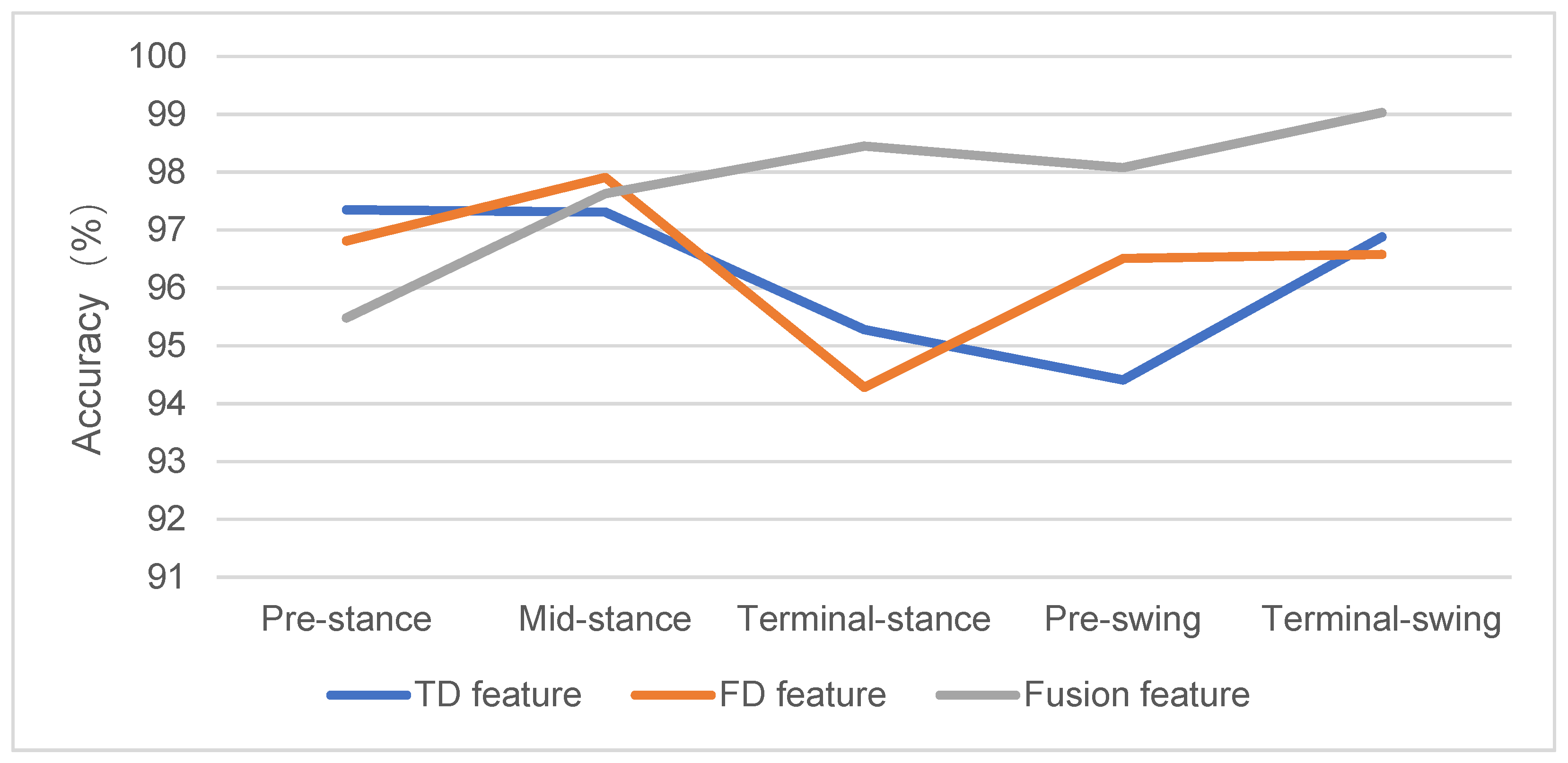
In order to study the influence of fusion features on classification performance as compared to using a single feature, the recognition rates of SSA-DBN under TD features, FD features, and fusion features are compared.

Figure 12 shows that the classification ability of an algorithm based on fusion features is significantly better than the use of single features. Second, the improvement in the classification ability of the swing phase is particularly significant under the fusion feature. This also proves that the fusion features can find more gait differences compared with the features in a single time domain or frequency domain, so as to better classify the five gait stages.

A comparison of DBN before and after optimization in time domain, frequency domain, and fusion feature dataset shows that the recognition rates of the five gait stages improve by different degrees after optimization. This shows that the SSA algorithm achieves the purpose of improving the classification accuracy of the DBN model by optimizing the weight parameters in the DBN model. This also proves that the SSA-DBN model is a real and effective model that can be applied to the actual gait classification problem.

4. Conclusions

In this paper, we optimized the deep belief network (DBN) by using the sparrow search algorithm (SSA) to perform gait classification based on multi-feature fusion of surface EMG signals. The DBN has the ability to find the distributed features of gait based on the underlying features. The use of the fused feature combination instead of single time domain or frequency domain features enables us to obtain higher classification accuracy and lower loss rate, and avoid the uncertainty caused by the traditional feature extraction. When the network structure and the parameters of DBN are changed manually and autonomously, the classification results change. Blindly increasing the number of fine-tunings may prolong the network training time and reduce the classification efficiency. The SSA is to optimize the parameters of the DBN model, such as the number of neurons in each layer, the learning rate, and the number of fine-tunings to aviod human-made interference. The experimental results show that SSA-DBN improves the gait recognition rate and stability. In addition, the SSA algorithm also increases the training time of the DBN network, while the optimization effect in some gait stages is limited. With the development of human gait detection and intelligent safety monitoring, the requirements for real-time classification are increasing, which lays the basis for our research direction in the future.

References

1. Wu, Z.; Huang, Y.; Wang, L.; Wang, X.; Tan, T. A comprehensive study on cross-view gait based human identification with deep CNNs. IEEE Trans. Pattern Anal. Mach. Intell. 2017, 39, 209–226. [Google Scholar] [CrossRef] [PubMed]
2. Roberts, M.; Mongeon, D.; Prince, F. Biomechanical parameters for gait analysis: A systematic review of healthy human gait. Phys. Ther. Rehabil. 2017, 4, 1–17. [Google Scholar] [CrossRef] [Green Version]
3. Bao, T.Z.; Zaidi, S.A.R.; Xie, S.Q.; Yang, P.F.; Zhang, Z.Q. A CNN-LSTM hybrid model for wrist kinematics estimation using surface electromyography. IEEE Trans. Instrum. Meas. 2021, 70, 2503809. [Google Scholar] [CrossRef]
4. Yao, T.; Gao, F.R.; Zhang, Q.Z.; Ma, Y.L. Multi-feature gait recognition with DNN based on sEMG signals. Math. Biosci. Eng. 2021, 18, 3521–3542. [Google Scholar] [CrossRef]
5. Alamri, A.; Cha, J.; El Saddik, A. Ar-rehab: An augmented reality framework for poststroke-patient rehabilitation. IEEE Trans. Instrum. Meas. 2010, 59, 2554–2563. [Google Scholar] [CrossRef]
6. Stenum, J.; Rossi, C.; Roemmich, R.T. Two-dimensional video-based analysis of human gait using pose estimation. PLoS Comput. Biol. 2021, 17, e1008935. [Google Scholar] [CrossRef]
7. Bijalwan, V.; Semwal, V.B.; Mandal, T.K. Fusion of multi-sensor-based biomechanical gait analysis using vision and wearable sensor. IEEE Sens. J. 2021, 21, 14213–14220. [Google Scholar] [CrossRef]
8. Ding, Y.R.; Pandala, A.; Li, C.Z.; Shin, Y.H.; Park, H.W. Representation-free model predictive control for dynamic motions in quadrupeds. IEEE Trans. Robot. 2021, 37, 1154–1171. [Google Scholar] [CrossRef]
9. Mustageem; Kwon, S. CLSTM: Deep feature-based speech emotion recognition using the hierarchical convLSTM network. Mathematics 2020, 8, 2133. [Google Scholar] [CrossRef]
10. Ye, M.X.; Yang, C.; Stankovic, V.; Stankovic, L.; Cheng, S. Distinct feature extraction for video-based gait phase classification. IEEE Trans. Multimed. 2020, 22, 1113–1125. [Google Scholar] [CrossRef]
11. Bai, X.R.; Hui, Y.; Wang, L.; Zhou, F. Radar-based human gait recognition using dual-channel deep convolutional neural network. IEEE Trans. Geosci. Remote Sens. 2019, 57, 9767–9778. [Google Scholar] [CrossRef]
12. Disselhorst-Klug, C.; Schmitz-Rode, T.; Rau, G. Surface electromyography and muscle force: Limits in sEMG-force relationship and new approaches for applications. Clin. Biomech. 2009, 24, 225–235. [Google Scholar] [CrossRef] [PubMed]
13. Gao, F.R.; Tian, T.X.; Yao, T.; Zhang, Q.Z. Human gait recognition based on multiple feature combination and parameter optimization algorithms. Comput. Intell. Neurosci. 2021, 2021, 6693206. [Google Scholar] [CrossRef] [PubMed]
14. Rainoldi, A.; Melchiorri, G.; Caruso, I. A method for positioning electrodes during surface EMG recordings in lower limb muscles. J. Neurosci. Methods 2004, 134, 37–43. [Google Scholar] [CrossRef] [PubMed]
15. Clark, D.J.; Ting, L.H.; Zajac, F.E.; Neptune, R.R.; Kautz, S.A. Merging of healthy motor modules predicts reduced locomotor performance and muscle coordination complexity post-stroke. J. Neurophysiol. 2010, 103, 844–857. [Google Scholar] [CrossRef] [PubMed] [Green Version]
16. Rueterbories, J.; Spaich, E.G.; Larsen, B.; Andersen, O.K. Methods for gait event detection and analysis in ambulatory systems. Med. Eng. Phys. 2010, 32, 545–552. [Google Scholar] [CrossRef] [PubMed]
17. Wei, P.N.; Xie, R.F.; Tang, R.N.; Li, C.; Kim, J.; Wu, M. sEMG based gait phase recognition for children with spastic cerebral palsy. Ann. Biomed. Eng. 2019, 47, 223–230. [Google Scholar] [CrossRef] [PubMed]
18. Pasluosta, C.F.; Gassner, H.; Winkler, J.; Klucken, J.; Eskofier, B.M. An emerging era in the management of Parkinson’s disease: Wearable technologies and the Internet of things. IEEE J. Biomed. Health Inform. 2015, 19, 1873–1881. [Google Scholar] [CrossRef] [PubMed]
19. Lin, Z.M.; Wu, Z.Y.; Zhang, B.B.; Wang, Y.C.; Guo, H.Y.; Liu, G.L.; Chen, C.Y.; Chen, Y.L.; Yang, J.; Wang, Z.L. A triboelectric nanogenerator-based smart insole for multifunctional gait monitoring. Adv. Mater. Technol. 2019, 4, 1800360. [Google Scholar] [CrossRef]
20. Benninger, D.H.; Berman, B.D.; Houdayer, E.; Pal, N.; Luckenbaugh, D.A.; Schneider, L.; Miranda, S.; Hallett, M. Intermittent theta-burst transcranial magnetic stimulation for treatment of Parkinson disease. Neurology 2011, 76, 601–609. [Google Scholar] [CrossRef]
21. Xi, X.; Tang, M.; Miran, S.M.; Luo, Z. Evaluation of feature extraction and recognition for activity monitoring and fall detection based on wearable sEMG sensors. Sensors 2017, 17, 1229. [Google Scholar] [CrossRef] [PubMed] [Green Version]
22. Qi, J.X.; Jiang, G.Z.; Li, G.F.; Sun, Y.; Tao, B. Surface EMG hand gesture recognition system based on PCA and GRNN. Neural Comput. Appl. 2020, 32, 6343–6351. [Google Scholar] [CrossRef]
23. Phinyomark, A.; Quaine, F.; Charbonnier, S.; Serviere, C.; Tarpin-Bernard, F.; Laurillau, Y. EMG feature evaluation for improving myoelectric pattern recognition robustness. Expert Syst. Appl. 2013, 40, 4832–4840. [Google Scholar] [CrossRef]
24. Felici, F.; Quaresima, V.; Fattorini, L.; Sbriccoli, P.; Filligoi, G.C.; Ferrari, M. Biceps brachii myoelectric and oxygenation changes during static and sinusoidal isometric exercises. J. Electromyogr. Kinesiol. 2009, 19, E1–E11. [Google Scholar] [CrossRef] [PubMed]
25. Hu, Q.; Qin, A.; Zhang, Q.; He, J.; Sun, G. Fault diagnosis based on weighted extreme learning machine with wavelet packet decomposition and KPCA. IEEE Sens. J. 2018, 18, 8472–8483. [Google Scholar] [CrossRef]
26. Sejdic, E.; Lowry, K.A.; Bellanca, J.; Redfern, M.S.; Brach, J.S. A comprehensive assessment of gait accelerometry signals in time, frequency and time-frequency domains. IEEE Trans. Neural Syst. Rehabil. Eng. 2014, 22, 603–612. [Google Scholar] [CrossRef] [Green Version]
27. Wei, P.N.; Zhang, J.H.; Tian, F.F.; Hong, J. A comparison of neural networks algorithms for EEG and sEMG features based gait phases recognition. Biomed. Signal Process. Control 2021, 68, 102587. [Google Scholar] [CrossRef]
28. Luo, R.M.; Sun, S.Q.; Zhang, X.F.; Tang, Z.C.; Wang, W.D. A low-cost end-to-end sEMG-based gait sub-phase recognition system. IEEE Trans. Neural Syst. Rehabil. Eng. 2020, 28, 267–276. [Google Scholar] [CrossRef]
29. Subasi, A. Classification of EMG signals using PSO optimized SVM for diagnosis of neuromuscular disorders. Comput. Biol. Med. 2013, 43, 576–586. [Google Scholar] [CrossRef] [PubMed]
30. Chen, X.P.; Zhang, D.G.; Zhu, X.Y. Application of a self-enhancing classification method to electromyography pattern recognition for multifunctional prosthesis control. J. Neuroeng. Rehabil. 2013, 10, 44. [Google Scholar] [CrossRef] [PubMed]
31. Wang, M.J.; Chen, H.L. Chaotic multi-swarm whale optimizer boosted support vector machine for medical diagnosis. Appl. Soft Comput. 2020, 88, 1–47. [Google Scholar] [CrossRef]
32. Youssef, A.M.; Pourghasemi, H.R. Landslide susceptibility mapping using machine learning algorithms and comparison of their performance at Abha Basin, Asir Region, Saudi Arabia. Geosci. Front. 2021, 12, 639–655. [Google Scholar] [CrossRef]
33. Shariati, M.; Mafipour, M.S.; Mehrabi, P.; Zandi, Y.; Dehghani, D.; Bahadori, A.; Shariati, A.; Trung, N.T.; Salih, M.N.A.; Poi-Ngian, S. Application of extreme learning machine (ELM) and genetic programming (GP) to design steel-concrete composite floor systems at elevated temperatures. Steel Compos. Struct. 2019, 33, 319–332. [Google Scholar]
34. Qi, J.X.; Jiang, G.Z.; Li, G.F.; Sun, Y.; Tao, B. Intelligent human-computer interaction based on surface EMG gesture recognition. IEEE Access 2019, 7, 61378–61387. [Google Scholar] [CrossRef]
35. Zhang, Q.Z.; Guo, B.; Kong, W.Z.; Xi, X.G.; Zhou, Y.Z.; Gao, F.R. Tensor-based dynamic brain functional network for motor imagery classification. Biomed. Signal Process. Control 2021, 69, 102940. [Google Scholar] [CrossRef]
36. Purushothaman, G.; Vikas, R. Identification of a feature selection based pattern recognition scheme for finger movement recognition from multichannel EMG signals. Australas Phys. Eng. Sci. Med. 2018, 41, 549–559. [Google Scholar] [CrossRef] [PubMed]
37. Zhao, X.H.; Zhang, X.; Cai, Z.N.; Tian, X.; Wang, X.Q.; Huang, Y.; Chen, H.L.; Hu, L.F. Chaos enhanced grey wolf optimization wrapped ELM for diagnosis of paraquat-poisoned patients. Comput. Biol. Chem. 2019, 78, 481–490. [Google Scholar] [CrossRef]
38. He, Z.Y.; Shao, H.D.; Zhang, X.Y.; Cheng, J.S.; Yang, Y. Improved deep transfer auto-encoder for fault diagnosis of gearbox under variable working conditions with small training samples. IEEE Access 2019, 7, 115368–115377. [Google Scholar] [CrossRef]
39. Merletti, R.; Farina, D.; Gazzoni, M.; Schieroni, M.P. Effect of age on muscle functions investigated with surface electromyography. Muscle Nerve 2002, 25, 65–76. [Google Scholar] [CrossRef]
40. Wang, J.; Gao, F.; Sun, Y.; Luo, Z. Non-uniform characteristics and its recognition effects for walking gait based on sEMG. Chin. J. Sens. Actuators 2016, 29, 384–389. [Google Scholar]
41. Kuremoto, T.; Kimura, S.; Kobayashi, K.; Obayashi, M. Time series forecasting using a deep belief network with restricted boltzmann machines. Neurocomputing 2014, 137, 47–56. [Google Scholar] [CrossRef]
42. Zhao, H.; Zheng, J.; Deng, W.; Song, Y. Semi-supervised broad learning system based on manifold regularization and broad network. IEEE Trans. Circuits Syst. I Regul. Pap. 2020, 67, 983–994. [Google Scholar] [CrossRef]
43. Liu, Y.; Wang, X.; Zhai, Z.; Chen, R.; Zhang, B.; Jiang, Y. Timely daily activity recognition from headmost sensor events. ISA Trans. 2019, 94, 379–390. [Google Scholar] [CrossRef] [PubMed]
44. Qiu, X.; Ren, Y.; Suganthan, P.N.; Amaratunga, G.A.J. Empirical mode decomposition based ensemble deep learning for load demand time series forecasting. Appl. Soft Comput. 2017, 54, 246–255. [Google Scholar] [CrossRef]
45. Hassan, M.M.; Alam, M.G.R.; Uddin, M.Z.; Huda, S.; Almogren, A.; Fortino, G. Human emotion recognition using deep belief network architecture. Inf. Fusion 2019, 51, 10–18. [Google Scholar] [CrossRef]
46. Lv, Z.; Qiao, L. Deep belief network and linear perceptron based cognitive computing for collaborative robots. Appl. Soft Comput. 2020, 92, 106300–106309. [Google Scholar] [CrossRef]
47. Samadi, F.; Akbarizadeh, G.; Kaabi, H. Change detection in SAR images using deep belief network: A new training approach based on morphological images. IET Image Process. 2019, 13, 2255–2264. [Google Scholar] [CrossRef]
48. Deng, W.; Liu, H.L.; Xu, J.J.; Zhao, H.M.; Song, Y.J. An improved quantum-inspired differential evolution algorithm for deep belief network. IEEE Trans. Instrum. Meas. 2020, 69, 7319–7327. [Google Scholar] [CrossRef]
49. Xue, J.K.; Shen, B. A novel swarm intelligence optimization approach: Sparrow search algorithm. Syst. Sci. Control. Eng. 2020, 8, 22–34. [Google Scholar] [CrossRef]
50. Li, J.; Wang, W.D.; Chen, G.; Han, Z. Spatiotemporal assessment of landslide susceptibility in Southern Sichuan, China using SA-DBN, PSO-DBN and SSA-DBN models compared with DBN model. Adv. Space Res. 2022, 69, 3071–3087. [Google Scholar] [CrossRef]
51. Vaughan, C.L.; Davis, B.; O’Conners, J.C. Dynamics of Human Gait, 3rd ed.; Human Kinetics: Champaign, IL, USA, 1992; pp. 15–43. [Google Scholar]
52. Au, S.K.; Weber, J.; Herr, H. Powered ankle–foot prosthesis improves walking metabolic economy. IEEE Trans. Robot. 2009, 25, 51–66. [Google Scholar] [CrossRef] [Green Version]
53. Phinyomark, A.; Nuidod, A.; Phukpattaranont, P.; Limsakul, C. Feature extraction and reduction of wavelet transform coefficients for EMG pattern classification. Elektron. Elektrotechnika 2012, 122, 27–32. [Google Scholar] [CrossRef]
54. Basahel, A.; Sattari, M.A.; Taylan, O.; Nazemi, E. Application of feature extraction and artificial intelligence techniques for increasing the accuracy of X-ray radiation based two phase flow meter. Mathematics 2021, 9, 1227. [Google Scholar] [CrossRef]
55. Mayet, A.M.; Nurgalieva, K.S.; Al-Qahtani, A.A.; Narozhnyy, I.M.; Alhashim, H.H.; Nazemi, E.; Indrupskiy, I.M. Proposing a high-precision petroleum pipeline monitoring system for identifying the type and amount of oil products using extraction of frequency characteristics and a MLP neural network. Mathematics 2022, 10, 2916. [Google Scholar] [CrossRef]
56. Parent, A.; Dal Maso, F.; Pouliot-Laforte, A.; Cherni, Y.; Marois, P.; Ballaz, L. Short walking exercise leads to gait changes and muscle fatigue in children with cerebral palsy who walk with jump gait. Am. J. Phys. Med. Rehabil. 2021, 100, 1093–1099. [Google Scholar] [CrossRef]
57. Hinton, G.E.; Osindero, S.; Teh, Y.W. A fast learning algorithm for deep belief nets. Neural Comput. 2006, 18, 1527–1554. [Google Scholar] [CrossRef]
58. Dong, X.T.; Li, Y.; Zhong, T.; Wu, N.; Wang, H.Z. Random and coherent noise suppression in DAS-VSP data by using a supervised deep learning method. IEEE Geosci. Remote Sens. Lett. 2022, 19, 8001605. [Google Scholar] [CrossRef]
59. McHugh, M.L. Standard error: Meaning and interpretation. Biochem. Med. 2008, 18, 7–13. [Google Scholar] [CrossRef]
60. Chia, K.; Sangeux, M. Quantifying sources of variability in gait analysis. Gait Posture 2017, 56, 68–75. [Google Scholar] [CrossRef]
Figure 1. The flowchart of the proposed method starting at obtaining the normal gait of the human body through to classifying the gait stages.
Mathematics 10 04387 g001
Figure 2. The partial muscle distribution of one subject in the lower limbs, including tensor fascia lata (TF), adductor longus (AL), rectus femoris (RF), vastus medialis (VM), tibialis anterior (TA), semitendinosus (ST), gastrocnemius (GM), and soleus (SO).
Mathematics 10 04387 g002
Figure 3. The gait cycle distribution, dividing preliminary gait stages by judging the position change of heel and toe.
Mathematics 10 04387 g003
Figure 4. The basic building module of DBN is RBM. (a) is composed of 1 RBM; (b) is composed of 2 RBMs; (c) is composed of n RBMs. The two arrows represent forward training and reverse fin e-tuning respectively.
Mathematics 10 04387 g004
Figure 5. The flowchart is divided into three parts, from right to left, the data processing part, the DBN model training part, and the SSA algorithm optimization model part. The double arrows indicate the transfer of parameters between SSA and DBN.
Mathematics 10 04387 g005
Figure 6. Original sEMG waveform. Eight channels of sEMG signals acquired in one gait cycle are marked with stance phase and swing phase.
Mathematics 10 04387 g006
Figure 7. The de-noising result of the selected lower limb muscle signal using the wavelet module maximum method. Taking the tensor fascia lata (TF) as an example, the red line represents the original signal before de-noising, and the blue line represents the signal after de-noising.
Mathematics 10 04387 g007
Figure 8. The time domain feature classification results.
Mathematics 10 04387 g008
Figure 9. The recognition rate curves for different fine-tuning times. The red line represents the recognition rate and the blue line represents the loss rate. (ad) respectively represent that fine-tunning time is 1, 20, 100, and 500.
Mathematics 10 04387 g009
Figure 10. The frequency domain feature recognition rate.
Mathematics 10 04387 g010
Figure 11. The fusion feature recognition rate.
Mathematics 10 04387 g011
Figure 12. A comparison of recognition rate under different features.
Mathematics 10 04387 g012