Article

Quantification of Aversion to Uncertainty in Intertemporal Choice through Subjective Perception of Time

Department of Mathematics and Physics, University of Campania Luigi Vanvitelli, Viale A. Lincoln, 5, 81100 Caserta, Italy
*
Author to whom correspondence should be addressed.
Mathematics 2022, 10(22), 4315; https://doi.org/10.3390/math10224315
Submission received: 22 October 2022 / Revised: 10 November 2022 / Accepted: 11 November 2022 / Published: 17 November 2022
(This article belongs to the Special Issue State-of-the-Art Mathematical Applications in Europe)

Abstract

:
Intertemporal choices are those decisions structured over several periods in which the effects only manifest themselves with the passage of time. The main mathematical reference for studying the behavior of individuals with respect to this type of decision is the Discounted Utility Model which hypothesizes completely rational individuals. The empirical evidence that deviates from normative expectations has motivated the formulation of alternative models with the aim of better describing the behavior of individuals. The present paper investigates the characteristics behind hyperbolic discounting starting from the phenomenon of decision inconsistency, i.e., when individuals’ preferences vary over time. The mechanisms of inconsistency will be explored through the physical concept of relative time, proving the importance of uncertainty aversion in the hyperbolic trend of the discount function. The analysis of the mathematical characteristics of hyperbolic discounting and the relationship between decision inconsistency and subjective perception of time defines the maximum distance between rational and non-rational preferences. An experimental part empirically proves the relationship between uncertainty aversion and time inconsistency. The present paper contributes to the literature by defining a new characteristic of hyperbolic discounting and quantifying the impact of the subjective perception of time in the decision-making process.

1. Introduction

Recent studies in finance argue that asset pricing should consider both risk and uncertainty [1]. The decision-making context in which the present research is developed involves choices under uncertainty, particularly the kind of decisions in which alternatives are distributed over time, called intertemporal choices. The purpose of the research is to understand how individuals behave when they have to select an intertemporal prospect from those available. The reason why intertemporal choices are so complex and interesting comes down to two characteristics. First, precisely because alternatives are spread over multiple periods, the selection of later and more important outcomes necessarily involves foregoing a more imminent and modest outcome [2]. Moreover, even after selecting an alternative, it is not necessarily perceived over time always to be the optimal one [3]. The essential mathematical reference model for the study of behavior with respect to intertemporal choices was formalized by Samuelson [4,5]. The model predicts that the utility of an alternative was calculated as the product between its cardinal utility and the discount function evaluated at the time of receipt. From an operational point of view, the discount function determines a reduction in the present utility of the outcome based on how the individual perceives the indeterminacy of the future. The first formulation of the model predicted an exponential trend in the discount function, in line with the principles of economic rationality, which assumes a perfectly rational decision-maker capable of considering all components of the decision-making environment. Empirical evidence has over time motivated research to formulate alternative discount functions that could better describe the behavior of individuals. The hyperbolic model was formalized later in response to the discrepancy between the preferences predicted by the exponential model and the behavior of individuals. The main difference between the hyperbolic model and the exponential model is that in the former, the discount rate and the degree of impatience [6] are not constant but decrease over time [7,8]. Initially, this feature of hyperbolic discounting came to be associated with a kind of non-rationality of decision-making, characterizing nonexponential preferences with a negative connotation. In 1957, the concept of bounded rationality introduced by Simon [9] proposed the idea of a decision-maker with limited cognitive ability and resources. A decision-maker applies her rationality only after simplifying the available alternatives not being able to perceive, from a cognitive point of view, their full complexity. The consequence of this mechanism is that the decision-making satisfies adequacy criteria to determine a satisfactory solution rather than identifying the absolute best alternative. Later, a variety of works [10,11] clarified that decision-making is affected by systematic distortions associated with cognitive machinery and the emotional sphere. Since everyone is prone to certain biases, the work on strategic personalization proposed in Nudge theory [12] and in behavioral personalized finance [13,14] highlights the importance of behavioral attitudes in decision-making. At this point, it is even more interesting to investigate the characteristics of hyperbolic discounting since it is an expression of the cognitive and behavioral structure of the decision-maker.
This paper aims to understand whether the decreasing discount rate and impatience are sufficient to describe the mechanisms underlying hyperbolic discounting, or whether there are concepts within its structure that have not yet been formalized. To achieve the purpose, the object under consideration in the present paper is the phenomenon of time inconsistency, for which an individual’s preferences vary over time. The idea is to describe the phenomenon of inconsistency by integrating within hyperbolic discounting the concept of subjective perception of time. Using a time transformation, a measure of inconsistency is defined to quantify the discrepancy between the exponential and hyperbolic models. The relationships between this new measure and the elements used so far to describe hyperbolic discounting (discount rate and impatience) will prove that it constitutes distinct and original elements from those found in the literature. A variety of works that operationally justify the present study [15,16,17,18,19,20,21,22] also lead one to associate the defined measure with an uncertainty aversion mechanism. The applicability of this research addresses the Markets in Financial Instruments Directive, 2014/65/UE (MiFID2), which emphasizes the need to create customer profiling to ensure personalized strategies and protection mechanisms. The quantification of bias through the concept of impatience [23] and the quantification of uncertainty aversion are two useful measures to define classes of behavioral investors. In fact, although this article is far from dealing with choices under risky conditions, uncertainty analysis is considered essential by some studies for asset pricing and entrepreneurship [24]. Therefore, any relationships between the measure presented in this article and risk aversion coefficients [25] could be topics for future research. Finally, the possibility of applying the measure presented in this paper to the strategic personalization and classification of individuals is supported by two well-known works in the literature: with respect to classification, [26] prove that there is a relationship between cognitive ability and hyperbolic discounting, with respect to customized strategic plans, on the other hand, [27] proves how it is possible to increase helper-control with techniques to reduce dynamically inconsistent preferences. This paper is organized as follows. After a brief presentation on the Discounted Utility Model, some studies are presented that justifies the introduction of a temporal transformation function in intertemporal choice theory. The problem of time inconsistency will shift from the trend of the discount function to the evaluation of perceived time. The new measure of inconsistency is characterized and discussed with respect to the discount factor and impatience exhibited by the function. An experimental part will empirically prove the formalized results. This is followed by a discussion and conclusion section.

2. Motivation and Mathematical Formalization

2.1. Discounted Utility Model and Time in Intertemporal Choice

Let x 1 , , x n be n alternatives available at the times t 1 , , t n , respectively. An intertemporal prospect is the n-pla ( x 1 , t 1 ; ; x n , t n ) of pairs ( x i , t i ) where x i , t i + . If the individual accepts the prospect, then the outcome x i will be received at time t i . The Discounted Utility Model [4,5] states that:
U ( x 1 , t 1 ; ; x n , t n ) = i = 0 n U x i f t i
where U x i is the cardinal utility of x i and f t i is the discount function. By definition, the discount function is defined as f : such that f 0 = 1 , f t monotonous decreasing and lim t f t = 0 . It is possible to prove that a discount function generates a relation, called preference relation ( ) , of total order and vice versa [6]. From a practical point of view, given ( x 1 , t 1 ; ; x n , t n ) and ( y 1 , s 1 ; ; y n , s n ) two different prospects then ( x 1 , t 1 ; ; x n , t n ) > f ( y 1 , s 1 ; ; y m , s m ) i = 0 n U ( x i ) f t i > i = 0 m U ( y i ) f s i and ( x 1 , t 1 ; ; x n , t n ) ~ f ( y 1 , s 1 ; ; y m , s m ) i = 0 n U ( x i ) f t i = i = 0 m U ( y i ) f s i : the first case indicates that the decision-making prefers to select the prospect ( x 1 , t 1 ; ; x n , t n ) ; the second case indicates that the decision-making is indifferent with respect the two prospects.
Preferences in intertemporal choice theory are weak order, continuous, monotone, and impatient [7]. The performance of the discount function is decisive for preferences because it determines a reduction in the present utility of the outcome according to the time distance between evaluation and reception. Table 1 reports the common discount functions in intertemporal choice theory.
As can be seen from Table 1, all discount functions have a decreasing trend over time, which, from a behavioral point of view, is equivalent to saying that in the future the value of an asset decreases because it is more uncertain. The main difference between the linear, exponential, and hyperbolic discount functions is that the first two decrease with a constant rate. In general, empirical evidence proves that hyperbolic discounting has greater descriptive power of individuals’ preferences than exponential discounting [28]. The psychological mechanisms underlying the decrease in the discount function are quantified by the discount rate and the degree of impatience. The discount rate, defined as ρ t = f t f t , represents “the proportional variation of f over a standard period” [8] (p. 425). The impatience of investor, defined in [ t i , t j ] is given by 1 f t j / f t i and represents “the amount of money that the agent is willing to lose in exchange for anticipating the availability of a $1 reward” [6] (p. 5). The main difference from a mathematical point of view between the exponential and hyperbolic formulation of the discount function lies in the fact that the discount rate and the degree of impatience are not constant over time in the hyperbolic discount. In particular, the degree with which impatience decreases represents the gap between preferring an event to occur and preferring an event to occur sooner [7].
Time is a concept that has attracted the curiosity of various fields of inquiry, such as philosophy and physics. Although the objective nature of time, associated with the chronological scanning of events, was obvious, the subjective perception of time is a dimension of human intuition that cannot be refuted. How the passage of time is perceived defines the cognitive, emotional, and motivational style of the individual [22,29]. As a result, decision-making is strongly influenced by the subjective perception of time. In intertemporal choices, in which the passage of time is critical to prospect evaluation, one must integrate the subjective perception of time into the dynamics responsible for the hyperbolic or exponential pattern of preferences. Regarding the key elements of the discounted Utility Model, a variety of studies prove the existence of a relationship between subjective perception of time, degree of impatience, and hyperbolic trends. Zauberman et al. [16] proved that the hyperbolic trend of the discount function decreases, considering the impact of subjective perception of time. Next, Nyberg et al. [17] verified that the decrease in impatience is correlated with a nonlinear perception of time. Among the mathematical formalization of the impact that the subjective perception of time has on decision-making, the discount function proposed by [30], named the general hyperbolic function, defines and includes the subjective time duration. The reference to a clear distinction between subjective time and physical time in intertemporal choice has been empirically proven by [31]. The present article, with respect to the cited literature, investigates the subjective perception of time as a physical component of hyperbolic discounting, determining a point of maximum temporal misperception that, to the best of our knowledge, had not yet been identified in the dynamics of decision inconsistency. This result also introduces the need to have to investigate the relationship that exists between impatience, discount rate (both decreasing over time), and temporal misperception since they have a different trends over time. From an operational point of view, the mathematical approach used in this paper is based on a time transformation function, referring to the theory of relativity. Dos Santos and Martinez [32] have already addressed inconsistency as the result of a subjective time dilation perception effect but unlike their study, the present work considers that time perceived by consistent functions is also a “proper time” different from objective time.
From a psychological perspective, the idea of introducing a time transformation to determine a measure of inconsistency that is associated with the subjective perception of time refers to the projection mechanism [18,19,20,21]. In practice, to evaluate the usefulness of an alternative available to a prospect, it is necessary to project the choice into the future. Therefore, defining a measure of inconsistency related to the subjective perception of time is equivalent to quantifying an individual’s aversion to the uncertainty of the future.

2.2. Aversion to Uncertainty and Inconsistency Function

Temporal inconsistency is the phenomenon whereby preferences vary over time. In practice, if the decision-maker has to choose between a smaller sooner outcome (SS) and a larger later outcome (LL), the choice will depend only on the discount applied. From a theoretical perspective, it is rational to prefer SS or LL, assuming that this preference remains constant over time. Inconsistency is generated when the decision-maker prefers LL at first and SS at a later evaluation time. This mechanism generates an intersection point between the hyperbolic and exponential functions.
Definition 1.
Let f t be a hyperbolic discount function. For each indifference pair of the type x , 0 ~ f y , t , y > x > 0 , the normative function is the exponential discount function y t such that x , 0 ~ y y , t .
Proposition 1.
Let f t be a hyperbolic discount function whose indifference x , 0 ~ y , T is fixed. Then, there is a unique normative function.
Proof. 
A generical exponential discount function can be expressed as y t = e z t , z 0 , + because δ ϵ 0 , 1 ! z 0 , + :   δ = 1 / e z . As z varies in 0 , + there are infinite exponential discount functions. The only exponential normative function that verifies Definition 1 is the one for z = ( ln x / y ) / T . □
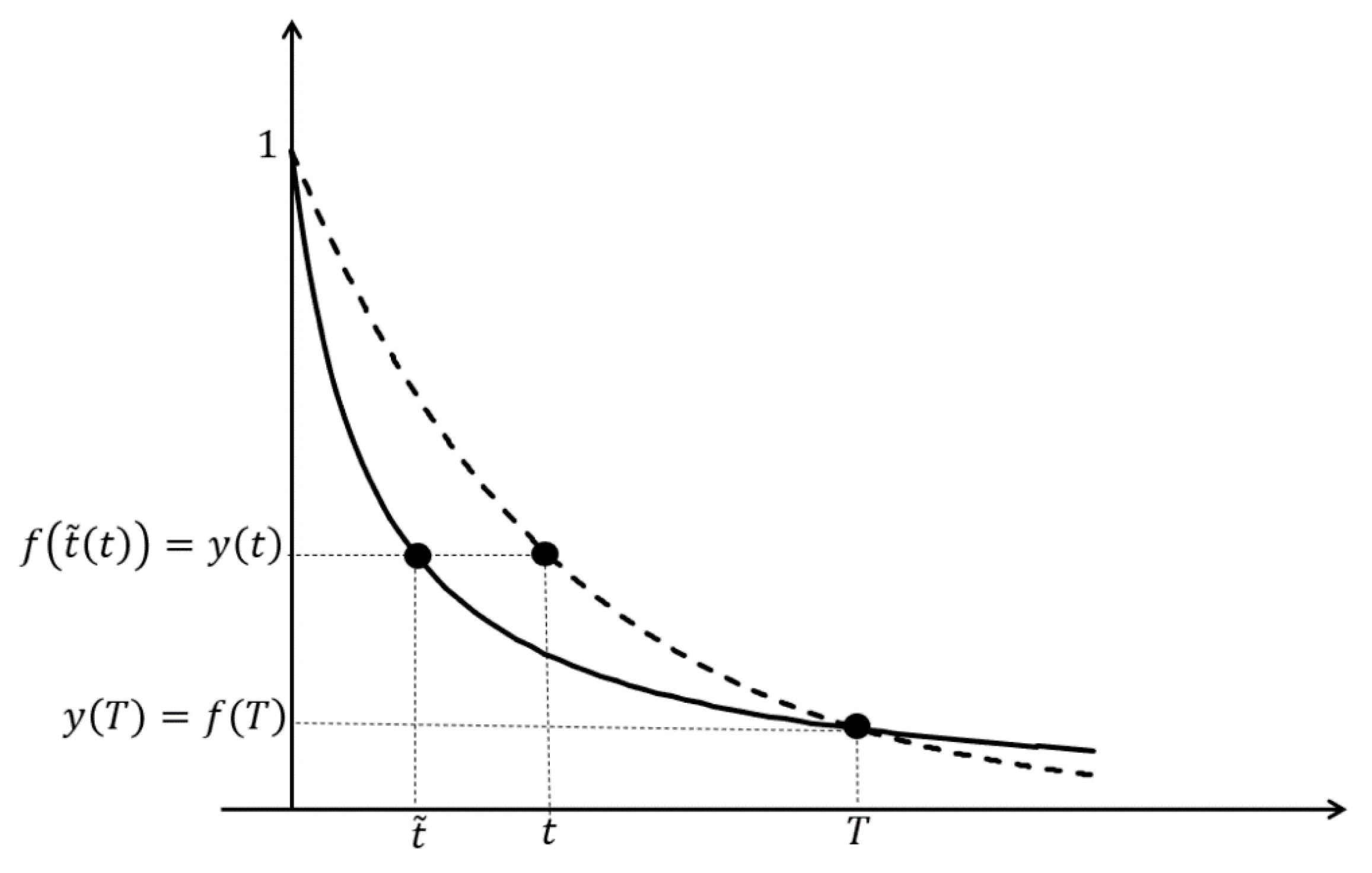
Figure 1 shows the relationship between the hyperbolic discount function and the related normative function for a generic indifference pair fixed at the time instant T . We observe that by the continuity property of the preference relation, it is sufficient to fix the initial outcome x to determine for each time instant the unique normative function.
Proposition 2.
Let f t be an exponential discount function and y t the respective exponential normative function then the time perceived by f t is shorter than that perceived by y t t 0 , T and it is longer than that perceived by t t T , + .
Proof. 
At the instant t = 0 , f t = y t = 1 . The existence of the point T such that f T = y T and the hyperbolic character of f t allows us to state that there exists at least one R > 0 in which f t has a steeper decrement than y t in a neighborhood I R 0 such that t < y t t 0 , T . From the monotony of the discount function ! t ˜ < t for which f t ˜ = y t . Thus, the generic instant t is perceived as if it were an instant closer to the origin, and the time perception of f t is contracted with respect to that of y t . For the interval T , + , the demonstration is analogous considering that f t > y t t T , + . □
Proposition 3.
Let y 1 t and y 2 t be two exponential normative functions of the hyperbolic discount function f t with respect to two indifference pairs x 1 , 0 ~ y 1 y 1 , T 1 and x 2 , 0 ~ y 2 y 2 , T 2 . If
ln x 1 y 1 T 1 > ln x 2 y 2 T 2
then the time perceived by y 1 t is longer than that perceived by y 2 t .
Proof. 
If 1 then z 1 < z 2 and δ 1 > δ 2 . What has been said is equivalent to state that t 0 , + , y 1 t > y 2 t . For the monotony of the discount function exists a point t ˜ < t such that y 1 t = y 2 t ˜ . The thesis follows as in Proposition 2. □
Definition 2.
Let f t and y t be a hyperbolic discount function and the respective exponential normative function. The time function between f t and y t is the function defined as:
t ˜ : 0 , + 0 , + t t ˜ t = t ˜
Proposition 4.
Let f t and y t be a hyperbolic discount function and the respective exponential normative function, then f t ˜ t = y t   t   0 , + .
Proof. 
Follows by Proposition 2. □
Figure 2 highlights the contraction mechanism described by the function t ˜ t .
Proposition 5.
Let y 1 t and y 2 t be two exponential normative functions of the hyperbolic discount function f t respect to x 1 , 0 ~ y 1 y 1 , t 1 and x 2 , 0 ~ y 2 y 2 , t 2 then t   0 , +   t t 1 ˜ t < t t 2 ˜ t y 1 t f t < y 2 t f t .
Proof. 
By hypothesis y 1 t < y 2 t . Let t 1 ˜ t and t 2 ˜ t be the time functions of f t with respect to y 1 t and y 2 t , respectively. t   0 , + y 1 t = f t 1 ˜ t < f t 2 ˜ t = y 2 t . For the monotony of f t t 1 ˜ t > t 2 ˜ t and follows the thesis.
⟹ By hypothesis t 1 ˜ t > t 2 ˜ t . The thesis follows from the monotony of f t . □
Definition 3.
Let f t and y t   be a hyperbolic discount function and the respective exponential normative function. The time misperception function d t ˜ and the empirical inconsistency function d y are defined as:
d t ˜ : 0 , + t t t ˜
d y : 0 , + t y t f t
Theorem 1.
Existence of maximum empirical inconsistency. Let f t and y t be a hyperbolic discount function and the respective exponential normative function then d y t admits at least one point of maximum in the interval 0 ,   T .
Proof. 
By construction d y 0 = f 0 y 0 = 0 and d y T = y T f T = 0 . As discussed in Proposition 2, t < y t t 0 , T . It follows that d y t is a continuous and positive function in the interval 0 , T . The thesis follows by considering that
lim t 0 d y t = lim t T d y t = 0
and d y t > 0 in 0 , T . □
Theorem 2.
Uniqueness of maximum empirical inconsistency. Let f t and y t be a hyperbolic discount function and the respective exponential normative function then d y t admits a unique point of maximum in the interval 0 ,   T .
Proof. 
Absurdly t 1 and t 2 are two points of maximum for the function d y t and without loss of generality t 1 < t 2 . By continuity of the function d y t , there exists a point t ^ : t 1 < t ^ < t 2 in which d y t reaches a minimum value. Then, we obtained that y t > f t t   0 , t 1 ,   y t < f t t   t 1 , t ^ and y t > f t t   t ^ , t 2 . The above contradicts the nature of the discount functions considered. □
This paper does not discuss the case of the interval T , + . Thus, although the properties of the discount function ensure the existence of a unique minimum m , it is not formalized.
Proposition 6.
Characterization of maximum empirical inconsistency. Let f t and y t be a hyperbolic discount function and the respective exponential normative function and let t 0 , T the maximum point for d y t . Denoted by ρ f = f t / f t and ρ y = y t / y t the discount rates of f t and y t then ! t ^   : t < t ^ < T for which ρ f t > ρ y ( t ) t 0 ,   t ^ and ρ f t < ρ y ( t ) t   t ^ , + .
Proof. 
By hypothesis t is the point of maximum for d y t , i.e., d d t y t f t t = t = 0 . It follows that y t f t = 0 . Since Proposition 2 and from the monotony of y t and f t follows that y t f t > 0 t   0 , t . In the interval 0 , t , y t > f t implies y t < f t and considering that d y t > 0 in 0 , T follows:
ρ f t = f t f t > y t y t = ρ y t
By Theorem 2, t f t < 0 t   t , m , with m the point of minimum of d y t . Since m > T then t f t < 0 t t , T , i.e., y T < f T . At the T -point, f T = y T :
ρ f T = f T f T < y T y T = ρ y T
Then, there exists a point t ^ > t such that ρ f t ^ = ρ y t ^ . The thesis follows considering that ρ y t is constant and ρ f t decreases. □
Proposition 7.
Let f t and y t be a hyperbolic discount function and the respective exponential normative function. The time misperception function d t ˜ increases (decreases) ⟺ empirical inconsistency function d y increases (decreases).
Corollary 1.
Let f t and y t be a hyperbolic discount function and the respective exponential normative function then t 0 , + is a maximum (or minimum) point for d t ˜ t t 0 , + is a maximum (or minimum) point for d y t .
Corollary 2.
Let f t and y t be a hyperbolic discount function and the respective exponential normative function then the time misperception function d t ˜ admits a unique point of maximum.
Proof. 
Follows by Theorem 1 and Theorem 2 and Corollary 1. □
Theorem 3.
Relationship between uncertainty and impatience. Let f t and y t be a hyperbolic discount function and the respective exponential normative function. Let t be the point in which the time misperception function d t ˜ reaches the maximum value then I f [ t i , t j ] > I y [ t i , t j ] t [ t i , t j 0 , t )   and I f [ t i , t j ] < I y [ t i , t j ] t [ t i , t j ] t , + .
Proof. 
By Proposition 6, t 0 ,   t it is possible to state that f t < y t . Let t i < t and h > 0 be such that t i + h = t j < t , then
f t = lim h 0 f t i + h f ( t i ) h < lim h 0 y t i + h y ( t i ) h = y t
f t i f ( t i + h ) f t i > f t i f ( t i + h ) y t i > y t i y ( t i + h ) y t i
I f [ t i , t j ] = 1 f ( t i + h ) f t i > 1 y ( t i + h ) y t i = I y [ t i , t j ]
The thesis follows from the assumption that f t = y t , and lim t i + I f [ t i , t j ] = 0 . □

3. Materials and Methods

Among the results proved in Section 2.2, the experimental phase refers in particular to the following objectives: to find the expression of the best empirical exponential function starting from a fixed initial outcome x , to analyze the correspondence between d t ˜ and d y function and their respective maximum points, to describe the variation of the sample’s uncertainty aversion, and to analyze the impatience trend of the hyperbolic discount function versus the exponential discount function. The questionnaire was implemented with the creation of a web application, made available and freely accessible by all Italian individuals. In fact, the test was designed entirely in Italian and voluntarily submitted only to Italian individuals to avoid the influence of cultural differences. The responses were stored in a database and processed for data analysis using Python and Excel. When uploading the link, the respondent had to indicate age and gender. Table 2 shows the distribution of the sample with a total of 50 individuals with respect to the characteristics considered.
The distribution of collected data is uneven with respect to age, probably due to the type of experimentation adopted (using a web app might be difficult or boring to an over-50 person). The distribution with respect to gender is uniform, but this article is not devoted to behavioral differences in the decision-making context between the two genders. This observation could be an additional line of development for the present research. After entering the characteristics shown in Table 2, the experiment includes an “INSTRUCTIONS” section, in which the response mode and the existence of time are briefly introduced. The questionnaire consists of two questions that alternate with each other: the first question is used to collect the values needed to construct the empirical discount function using the interpolation technique; the second question is used to elicit a sense of confusion. The first question answers the following:
“You have to receive U x t i euros in t i days, how much do you want to receive in t i + 1 days to consider the offer equivalent?”
The second question, used as distraction, is like the previous one but leaves the figure constant over time as follows:
“You have to receive 100 euros today, how much do you want to receive in t i days to consider the offer equivalent?”
In this way, it will be more difficult for respondents to keep track of the figures they write previously in response to the first question. Individuals undergoing the experimental phase did not actually receive the proposed figures but were asked to respond hypothetically. In this regard, from an experimental point of view [33] proves that decision-making processes may vary whether the money figures are real or hypothetical. However, because the application of the present article is especially directed toward empirical testing of theoretically proven results, it is not interested in investigating the influence of decision context in the proposed inconsistency measure, although this may be a future avenue of research. The initial outcome has been set as U x 0 = 100 , a moderate amount to enable individuals of all ages to realize the hypothesis in a practical way. For each question, the maximum time to answer was set at 20 s, and the countdown was constantly visible in a square placed below the question. In this way, each respondent had a constant perception of the limited passage of time. This dynamic was designed to elicit haste and agitation from each respondent. At the end of the countdown, if the question had not yet been submitted, the statement.
“Time’s up! The time available to answer the question has expired. Please answer the question IMMEDIATELY without further thought.”
Would appear on the website. The introductory display also points out that if the time expires more than 10 times, the sample analyzed will be disregarded. Fortunately, all individuals who participated fell within the imposed limit of 10 countdown deadlines.
The time instants for defining indifference pairs are t = 0 ,   2 ,   4 ,   7 ,   10 ,   14 ,   20 ,   30 ,   45 ,   60 ,   90 . The choice of heterogeneous intervals is related to the need to preserve homogeneity in the perception of the future (for example, the interval 4 ,   6 is perceived equivalently to the interval 4 ,   7 but the interval 6 ,   10 is not perceived as the interval 10 ,   14 ).
The discount function was obtained by interpolating the median values of individual participants as:
f t = f 0 = 1 f t i + 1 = f t i U x t i U x t i + 1
The choice of median depends on the high variability of the results obtained at the end of the interviews (e.g., f 20 0.000067 ; 33.33 ).

4. Results

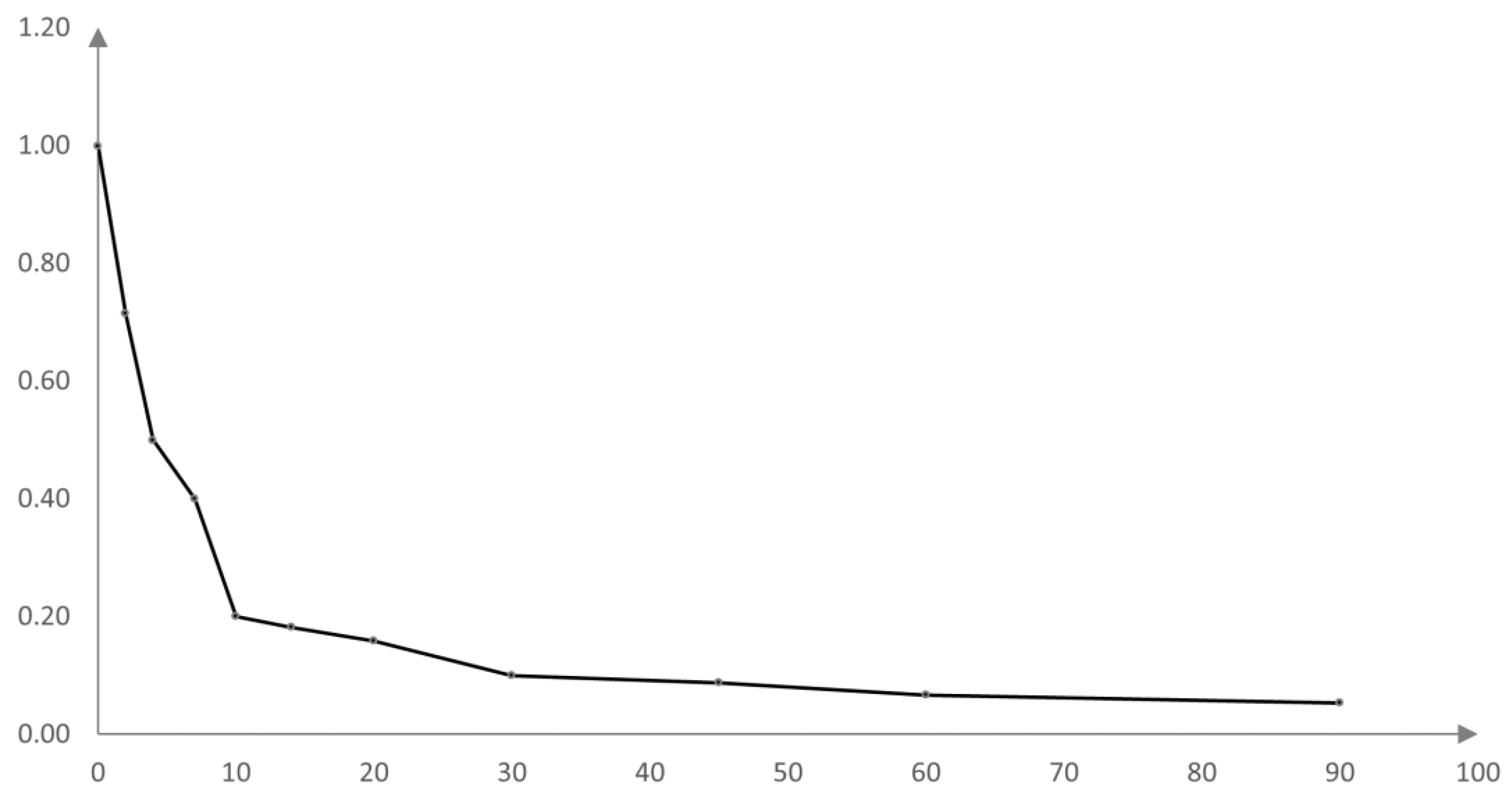
Figure 3 represents the obtained discount function, in which a steeper initial discount, characteristic of the empirical evidence and hyperbolic discounting, is shown.
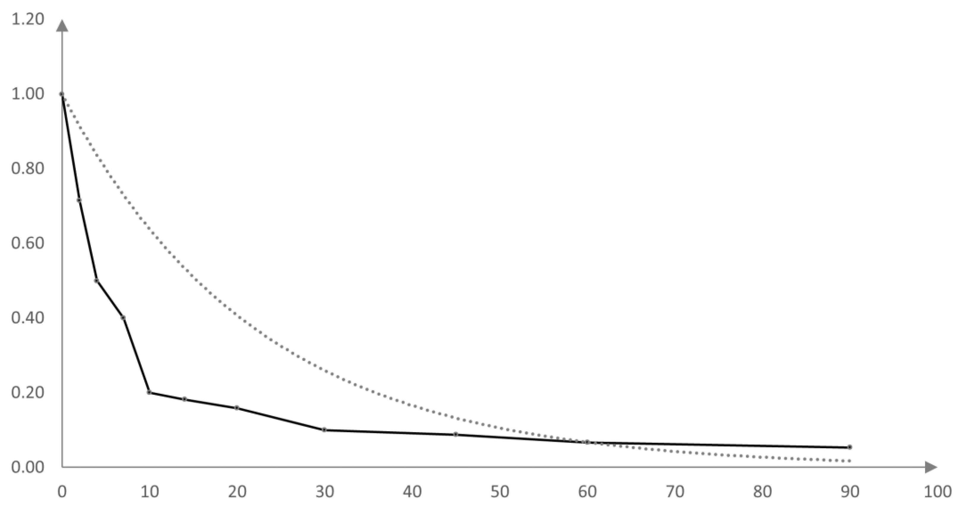
To determine the normative exponential function, instead of fixing a priori a point T needed for definition, the best exponential approximation of the empirical curve was evaluated with Excel, obtaining T = 60 . Any other point chosen would still have defined a single normative exponential function, but this strategy minimizes the maximum discrepancy between the exponential and hyperbolic trends. The normative exponential function occurs for z = 0.045 and its trend is shown in Figure 4.
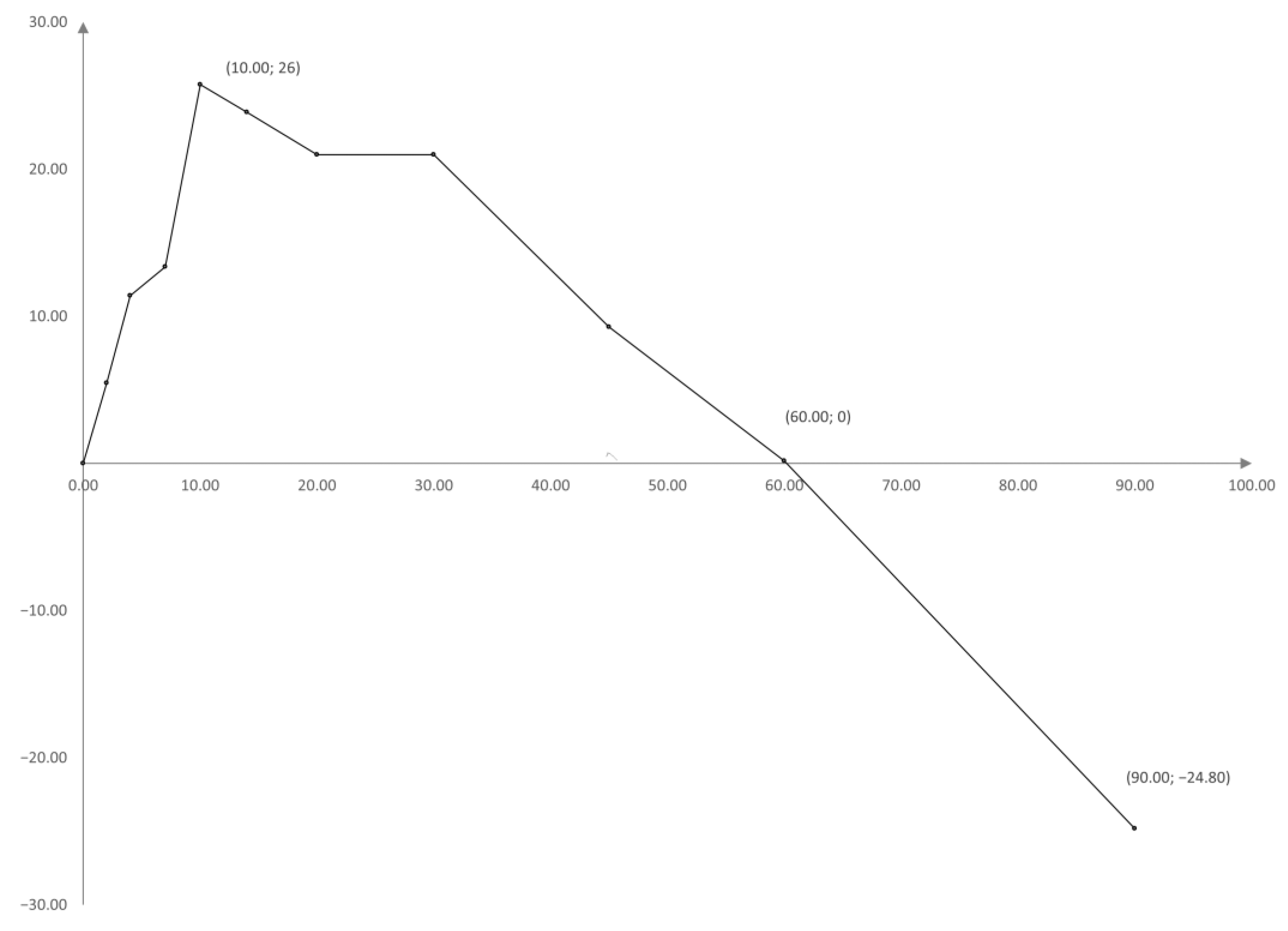
The function, representing the discrepancy between exponential preferences and hyperbolic trends, was calculated as in Definition 3. The graph is shown in Figure 5.
To check the correspondence between the point at which the maximum discrepancy occurs and the point at which the maximum contraction to the future occurs, identified by the point at which the maximum of the temporal misperception function occurs, the function d t ˜ t was calculated. The graph is shown in Figure 6.
For the construction of the graph of d t ˜ t , it was assumed that the time perceived by the sample is that associated with the hyperbolic curve. Therefore, the time of the exponential discount function was calculated by the inverse formula:
t ˜ 1 t = ln f t 0.045
It is possible to observe that the point at which the functions d t ˜ t and d y t reach the maximum value is for both functions t = 10 . The importance of t = 10 is also evident in Table 3, which confirms the result proved in Theorem 3. In fact, I f [ t i , t j ] > I y [ t i , t j ] before the point t = 10 and then the situation changes. This result is an empirical evidence of the relationship between the quantities used so far to describe inconsistency and the measure proposed by this paper. In addition, this result confirms that individuals who apply hyperbolic discounting exhibit greater impatience in periods closer to the present than those who apply exponential discounting.

5. Discussion

Intertemporal choices have a great influence on everyday life [34]. The discrepancy between the normative model and empirical evidence has motivated researchers to investigate the dynamics of decision-making when alternatives distributed over multiple periods are evaluated. The mechanisms of hyperbolic discounting, a reflection of the human rationality of the decision-maker, have so far been described through the discount factor and the degree of impatience.
This paper deepens the characteristics of hyperbolic discounting by adding a third element to the study of preference trends: time perception. The idea behind the definitions presented in Section 2.2 is to shift the problem of time inconsistency, a phenomenon associated with hyperbolic discount function performance, from curve performance to time perception. The transformation defined in Definition 2 made it possible to derive a new characteristic of hyperbolic discounting. In fact, although the two functions coincide punctually (Proposition 4), the discrepancy between hyperbolic and exponential preferences increases to a point of maximum. The existence of a maximum point is a feature not associated with either the degree of impatience or the discount rate, both of which assume a decreasing trend over time. The correspondence between the trend of the functions, proven in Corollary 1, justifies the idea of considering a psychological relationship between the two maximum points. In this regard, the present work addresses the mechanism of projection into the future that occurs when an intertemporal prospect is evaluated. The temporal contraction of perceived time invokes a dynamic of contraction that the individual feels with respect to the future. The aversion the decision-maker feels with respect to the future increases over time because it is more distant and because it is more difficult to imagine [35]. The existence of the maximum is when the individual becomes emotionally disinterested in a scenario that she cannot yet perceive (as if it were a future too far in the future to feel concerned and to imagine its projection sharply). Therefore, the degree of uncertainty aversion begins to decrease, and so the discrepancy between the hyperbolic and exponential functions does the same. The dynamic described is equivalent to saying that the decision-maker is more uncertainty averse, for example, to a future that is 10 days away, rather than 5 years away. Again, cognitive limitations and the emotional factor of the decision-maker are responsible for what is observed. The relationships tested with respect to the discount factor and impatience (Proposition 6 and Theorem 3) show that they are all distinct objects expressing three different dynamics: the discount factor expresses how much one prefers an event to happen, impatience expresses how much one prefers an event to happen sooner, and uncertainty aversion expresses how close one perceives the future to be.
The experimental phase empirically confirmed the results proven in Section 2. With respect to the implementation of the experiment, it is possible to observe how simple the construction of the proposed measure is. In fact, once the discount function is obtained through the interpolation technique, the construction of the best exponential function that approximates it is imminent even using simple Excel spreadsheets. Therefore, the proposed inconsistency measure lends itself to a very wide audience of researchers, who can investigate the dynamics of decision-making in intertemporal choices by varying the time instants considered, the lengths of the intervals, the initial digit, and so on, without necessarily making use of advanced implementation techniques. So far, the calculation of the degree of inconsistency of a discount function has always been a much-discussed problem, especially since [7] formalized the measure of the degree of decrease in impatience, defined as D I t = ln f t l n   f t . The proposed measure, in fact, is very difficult to calculate from an empirical point of view since it requires the calculation of the first and second derivatives of the logarithm. Subsequently, the following works deepened the tool proposed by [7] by improving its quantitative aspect: [36], through the introduction of time trade-off curves, generally simplified both qualitative and quantitative analysis of inconsistency; [37], on the other hand, formalized the concept of hyperbolic factor that provides the degree of decrease in impatience fixed an indifference pair.
The measure formalized in the present paper does not replace those mentioned but complements them because it conceptually differs from the psychological mechanisms incorporated in the concept of decreasing impatience, but still turns out to be a description of it, as proved in Theorem 3. Particularly important is the correspondence between Figure 5 and Figure 6 and Table 3, in which the point t = 10 is critical. What has been observed should not be surprising considering that the same measure defined by Prelec, can be described as D I t = ln ρ t . The expression is equivalent to saying that the rate at which the discount rate varies is related to the degree to which impatience decreases, and the way in which the discount rate varies, by definition, quantifies how the individual’s perception of the indeterminacy of time changes. In conclusion, the novelty of the measure of inconsistency proposed by the present paper lies in being characterized by a maximum point that represents the boundary between the emotional drive and the detachment from it of the decision-maker.

6. Conclusions

This article refers to the investigation of the discrepancy between normative models and empirical evidence in the context of intertemporal choices. The characteristics of hyperbolic discounting, starting from inconsistency, were explored through the concept of subjective perception of time. A dynamic related to how the decision-maker perceives the remoteness of the future was quantified. This mechanism generates a contraction with respect to the time frames involved in the intertemporal prospect and contributes to the hyperbolic preference trend. An experimental phase empirically confirmed the proven results. The research conducted aims at three key concepts: anomaly, normalization, and personalization.
The term anomaly denotes those phenomena that are difficult to rationalize from a theoretical point of view. The anomalies of the Discounted Utility Model [38,39] are described by a hyperbolic trend of the discount function. The goal is the full description of the anomalies through a combination of the quantities mentioned throughout the paper (impatience, discount rate, uncertainty, and subjective time).
Quantifying the gap between the normative model and the empirical evidence allows the normalization of anomalous attitudes, defining the extent to which the decision-maker’s bounded rationality respects economic rationality, also overcoming from a formal point of view the concept of non-rationality. These first two key concepts are unified in personalization: after understanding and quantifying non-rational preferences, these measures can be used to define classes of investors. The need to introduce personalized strategies is known from the work of Pompian [13,14] and Thaler [12]: the former refers to personalization by behavioral attitudes; the latter discusses systematic cognitive alterations in decision-making and projects them into a strategic architecture. In addition, the planning ability of individuals is not common to all decision-makers but is related to cognitive ability [26] and is critical to reducing the effects of myopic behavior in the future [27]. Therefore, quantifying the elements of the hyperbolic discount, which represents the expression of the individual’s decision-making process, is a method for calibrating the personalized approach.
The need to concretize these tools responds to the Markets in Financial Instruments Directive, 2014/65/UE (MiFID2) which emphasizes the need to consider the client’s needs, but also her behavioral attitudes with respect to available alternatives. Specifically, MiFID 2 can be seen as a tool to protect savers by requiring client assessment mechanisms. The main goal is to achieve a maximum fit between the individual’s profile and the products offered. In assessing suitability, customer profiling addresses both objective and subjective characteristics of the individual: objective characteristics include, for example, criteria such as investment objectives, duration of service, and associated risks; subjective characteristics, on the other hand, are all behavioral and individual aspects of the customer such as risk tolerance, knowledge needed to understand portfolio assets, and financial situation. Only by increasing the details that describe the client’s profile, recommendable financial instruments can be determined.
The measure proposed in the present paper refers to the subjective aspect of customer traits. First, quantifying the impact that subjective time has on intertemporal preferences can help investigate investor attitudes toward debt and investment dynamics [40], through the anomalies of the intertemporal choices [38,39]. The above could provide an additional criterion, in addition to personality traits [41,42], for the classification required by MiFID 2. With respect to the emotional sphere, on the other hand, the proposed measure of inconsistency, because it expresses the subjective perception of time, is linked related to emotional factors that interact with decision-making [43,44] and can help investigate the relationship between investor sentiment and financial activity [45]. For example, assuming risk as a feeling [46], assessing the influence of subjective time in the description of decision inconsistency can improve the description of risk aversion and perception of risk [47,48,49], elements on which MiFID 2 places so much emphasis on when designing customized plans. The transition between measurement and individualized plan design can be guided using decision support techniques, such as multicriteria methods [50,51].
From a conceptual point of view, one possible development of this paper is the introduction of another concept fundamental for calibrating strategies, financial inertia [52]. Inertia in finance, as in physics, is the force by which a body, in this case the investor, opposes a change in its motion. In this sense, inertia, as a force, helps delineate the geometric properties of the curve associated with the discount function. Finally, in addition to extending the formalization to the other anomalies of the Discounted Utility Model [38,39], it would be interesting to discuss the measure in a continuous, not discrete set of definitions. For although intertemporal choice is determined by precise instants of time, the concept of uncertainty aversion is continuous over time, and its extension in this sense could enhance its descriptive capabilities of the psychological mechanisms responsible.

Author Contributions

All authors contributed equally to this work. All authors have read and agreed to the published version of the manuscript.

Funding

This research received no external funding.

Institutional Review Board Statement

Not applicable.

Informed Consent Statement

Informed consent was obtained from all subjects involved in the study.

Data Availability Statement

Not applicable.

Conflicts of Interest

The authors declare no conflict of interest.

References

  1. Anderson, E.W.; Ghysels, E.; Juergens, J.L. The impact of risk and uncertainty on expected returns. J. Financ. Econ. 2009, 94, 233–263. [Google Scholar] [CrossRef] [Green Version]
  2. Noor, J. Intertemporal choice and the magnitude effect. Games Econ. Behav. 2011, 72, 255–270. [Google Scholar] [CrossRef]
  3. Sayman, S.; Öncüler, A. An investigation of time inconsistency. Manag. Sci. 2009, 55, 470–482. [Google Scholar] [CrossRef] [Green Version]
  4. Samuelson, P.A. A note on measurement of utility. Rev. Econ. Stud. 1937, 4, 155–161. [Google Scholar] [CrossRef]
  5. Samuelson, P.A. Probability, utility, and the independence axiom. Econom. J. Econom. Soc. 1952, 20, 670–678. [Google Scholar] [CrossRef]
  6. Cruz Rambaud, S.; Muñoz Torrecillas, M.J. Measuring impatience in intertemporal choice. PLoS ONE 2016, 11, e0149256. [Google Scholar] [CrossRef] [Green Version]
  7. Prelec, D. Decreasing impatience: A criterion for Non-stationary time preference and “hyperbolic” discounting. Scand. J. Econ. 2004, 106, 511–532. [Google Scholar] [CrossRef]
  8. Read, D. Blackwell Handbook of Judgment and Decision Making; John Wiley & Sons: Hoboken, NJ, USA, 2008; pp. 424–443. [Google Scholar]
  9. Simon, H.A. Models of Man, Social and Rational: Mathematical Essays on Rational Human Behavior in Society Setting; Wiley: New York, NY, USA, 1957. [Google Scholar]
  10. Kahneman, D. Thinking, Fast and Slow; Farrar, Straus and Giroux: New York, NY, USA, 2011. [Google Scholar]
  11. Kahneman, D.; Tversky, A. Prospect theory: An analysis of decision under risk. In Handbook of the Fundamentals of Financial Decision Making: Part I; World Scientific: Singapore, 2013; pp. 99–127. [Google Scholar]
  12. Thaler, R.H.; Sunstein, C.R. Nudge: Improving Decisions about Health, Wealth, and Happiness; Reviewed and Expanded Edition; Penguin Books: New York, NY, USA, 2009. [Google Scholar]
  13. Pompian, M.M. Using behavioral investor types to build better relationships with your clients. J. Financ. Plan. 2008, 21, 64–76. [Google Scholar]
  14. Pompian, M.M. Behavioral Finance and Investor Types: Managing Behavior to Make Better Investment Decisions; John Wiley & Sons: Hoboken, NJ, USA, 2012. [Google Scholar]
  15. Agostino, C.S.; Claessens, P.M.E.; Balci, F.; Zana, Y. The role of time estimation in decreased impatience in intertemporal choice. J. Neurosci. Psychol. Econ. 2021, 14, 185. [Google Scholar] [CrossRef]
  16. Zauberman, G.; Kim, B.K.; Malkoc, S.A.; Bettman, J.R. Discounting time and time discounting: Subjective time perception and intertemporal preferences. J. Mark. Res. 2009, 46, 543–556. [Google Scholar] [CrossRef]
  17. Nyberg, L.; Kim, A.S.N.; Habib, R.; Levine, B.; Tulving, E. Consciousness of subjective time in the brain. Proc. Natl. Acad. Sci. USA 2010, 107, 22356–22359. [Google Scholar] [CrossRef] [PubMed]
  18. Loewenstein, G. Out of control: Visceral influences on behavior. Organ. Behav. Hum. Decis. Process. 1996, 65, 272–292. [Google Scholar] [CrossRef] [Green Version]
  19. Loewenstein, G.; O’Donoghue, T.; Rabin, M. Projection bias in predicting future utility. Q. J. Econ. 2003, 118, 1209–1248. [Google Scholar] [CrossRef] [Green Version]
  20. Loewenstein, G.; Prelec, D.; Shatto, C. Hot/Cold Intrapersonal Empathy Gaps and the under-Prediction of Curiosity. Unpublished Manuscript; Carnegie-Mellon University: Pittsburgh, PA, USA, 1998. [Google Scholar]
  21. Wheeler, M.A.; Stuss, D.T.; Tulving, E. Toward a theory of episodic memory: The frontal lobes and autonoetic consciousness. Psychol. Bull. 1997, 121, 331. [Google Scholar] [CrossRef] [PubMed]
  22. Zimbardo, P.; Boyd, J. The Time Paradox: The New Psychology of Time that Will Change Your Life; Simon and Schuster: New York, NY, USA, 2008. [Google Scholar]
  23. Ventre, V.; Rambaud, S.C.; Martino, R.; Maturo, F. An analysis of intertemporal inconsistency through the hyperbolic factor. Qual. Quant. 2022, 1–28. [Google Scholar] [CrossRef]
  24. Gifford, S. Risk and uncertainty. In Handbook of Entrepreneurship Research; Springer: Boston, MA, USA, 2003; pp. 37–53. [Google Scholar]
  25. LeRoy, S.F.; Werner, J. Principles of Financial Economics; Cambridge University Press: Cambridge, MA, USA, 2014. [Google Scholar]
  26. Da Silva, S.; De Faveri, D.; Correa, A.; Matsushita, R. High-income consumers may be less hyperbolic when discounting the future. Economics Bulletin. 2017, 37, 1421–1434. [Google Scholar]
  27. Laibson, D. Golden eggs and hyperbolic discounting. Q. J. Econ. 1997, 112, 443–478. [Google Scholar] [CrossRef] [Green Version]
  28. Green, L.; Myerson, J.; McFadden, E. Rate of temporal discounting decreases with amount of reward. Mem. Cogn. 1997, 25, 715–723. [Google Scholar] [CrossRef]
  29. Shipp, A.J.; Edwards, J.R.; Lambert, L.S. Conceptualization and measurement of temporal focus: The subjective experience of the past, present, and future. Organ. Behav. Hum. Decis. Processes 2009, 110, 1–22. [Google Scholar] [CrossRef]
  30. Takahashi, T. Loss of self-control in intertemporal choice may be attributable to logarithmic time-perception. In Behavioral Economics of Preferences, Choices, and Happiness. Med. Hypotheses 2005, 65, 691–693. [Google Scholar] [CrossRef] [Green Version]
  31. Han, R.; Takahashi, T. Psychophysics of time perception and valuation in temporal discounting of gain and loss. Phys. A Stat. Mech. Its Appl. 2012, 391, 6568–6576. [Google Scholar] [CrossRef]
  32. Dos Santos, L.S.; Martinez, A.S. Inconsistency and subjective time dilation perception in intertemporal decision making. Front. Appl. Math. Stat. 2018, 4, 54. [Google Scholar] [CrossRef]
  33. Xu, S.; Xiao, Z.; Rao, H. Hypothetical versus real monetary reward decrease the behavioral and affective effects in the Balloon Analogue Risk Task. Exp. Psychol. 2019, 66, a000447. [Google Scholar] [CrossRef] [PubMed]
  34. Lu, Y.; Yang, C. Measuring impatience: Experiments of intertemporal choices. In Education Management and Management Science; CRC Press: Boca Raton, FL, USA, 2015; pp. 311–314. [Google Scholar]
  35. Gilbert, D.T.; Gill, M.J.; Wilson, T.D. The future is now: Temporal correction in affective forecasting. Organ. Behav. Hum. Decis. Processes 2002, 88, 430–444. [Google Scholar] [CrossRef] [Green Version]
  36. Attema, A.E.; Bleichrodt, H.; Rohde, K.I.; Wakker, P.P. Time-tradeoff sequences for analyzing discounting and time inconsistency. Manag. Sci. 2010, 56, 2015–2030. [Google Scholar] [CrossRef] [Green Version]
  37. Rohde, K.I. The hyperbolic factor: A measure of time inconsistency. J. Risk Uncertain. 2010, 41, 125–140. [Google Scholar] [CrossRef] [Green Version]
  38. Loewenstein, G.; Thaler, R.H. Anomalies: Intertemporal choice. J. Econ. Perspect. 1989, 3, 181–193. [Google Scholar] [CrossRef] [Green Version]
  39. Loewenstein, G.; Prelec, D. Anomalies in intertemporal choice: Evidence and an interpretation. Q. J. Econ. 1992, 107, 573–597. [Google Scholar] [CrossRef] [Green Version]
  40. Hoang, E.C.; Hoxha, I. Corporate payout smoothing: A variance decomposition approach. J. Empir. Financ. 2016, 35, 1–13. [Google Scholar] [CrossRef]
  41. Conlin, A.; Kyröläinen, P.; Kaakinen, M.; Järvelin, M.R.; Perttunen, J.; Svento, R. Personality traits and stock market participation. J. Empir. Financ. 2015, 33, 34–50. [Google Scholar] [CrossRef] [Green Version]
  42. Tauni, M.Z.; Fang, H.X.; Yousaf, S. The influence of investor personality traits on information acquisition and trading behavior: Evidence from Chinese futures exchange. Personal. Individ. Differ. 2015, 87, 248–255. [Google Scholar] [CrossRef]
  43. McLoughlin, A. Factors Affecting Human Time Perception: Do Feelings of Rejection Increase the Rate of Subjective Timing? Timing Time Percept. 2019, 7, 131–147. [Google Scholar] [CrossRef]
  44. Droit-Volet, S.; Meck, W.H. How emotions colour our perception of time. Trends Cogn. Sci. 2007, 11, 504–513. [Google Scholar] [CrossRef]
  45. Schmeling, M. Investor sentiment and stock returns: Some international evidence. J. Empir. Financ. 2009, 16, 394–408. [Google Scholar] [CrossRef] [Green Version]
  46. Loewenstein, G.F.; Weber, E.U.; Hsee, C.K.; Welch, N. Risk as feelings. Psychol. Bull. 2001, 127, 267. [Google Scholar] [CrossRef] [PubMed]
  47. Wang, M.; Keller, C.; Siegrist, M. The less You know, the more You are afraid of—A survey on risk perceptions of investment products. J. Behav. Financ. 2011, 12, 9–19. [Google Scholar] [CrossRef]
  48. Broihanne, M.H.; Merli, M.; Roger, P. Overconfidence, risk perception and the risk-taking behavior of finance professionals. Financ. Res. Lett. 2014, 11, 64–73. [Google Scholar] [CrossRef]
  49. Sun, Y.; Li, S. The effect of risk on intertemporal choice. J. Risk Res. 2010, 13, 805–820. [Google Scholar] [CrossRef]
  50. Toloie-Eshlaghy, A.; Homayonfar, M. MCDM methodologies and applications: A literature review from 1999 to 2009. Res. J. Int. Stud. 2011, 21, 86–137. [Google Scholar]
  51. Saaty, T.L. Decision making—The analytic hierarchy and network processes (AHP/ANP). J. Syst. Sci. Syst. Eng. 2004, 13, 1–35. [Google Scholar] [CrossRef]
  52. Gal, D. A psychological law of inertia and the illusion of loss aversion. Judgm. Decis. Mak. 2006, 1, 23–32. [Google Scholar]
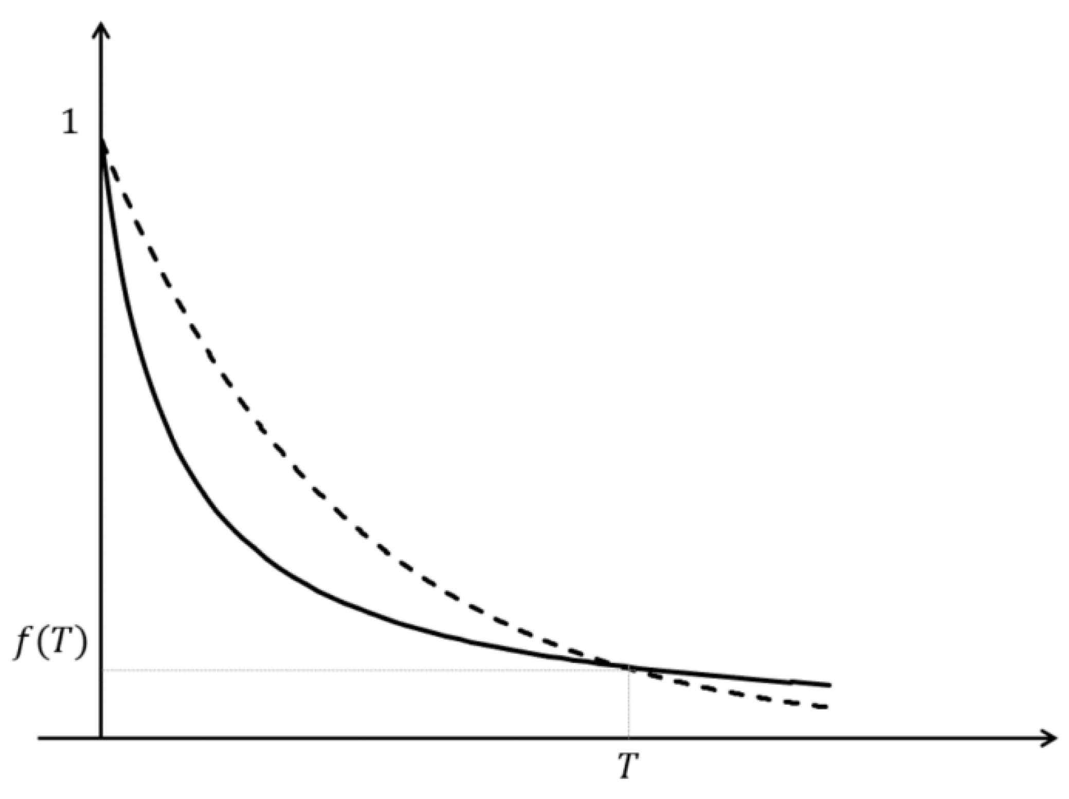
Figure 1. Representation of a hyperbolic discount function and the related empirical function.
Mathematics 10 04315 g001
Figure 2. Correspondence between the function t ˜ t and the time scanned by exponential discounting.
Mathematics 10 04315 g002
Figure 3. Discount function obtained from interview collection.
Mathematics 10 04315 g003
Figure 4. Empirical and normative functions.
Mathematics 10 04315 g004
Figure 5. Graph of d y t .
Mathematics 10 04315 g005
Figure 6. Graph of d t ˜ t .
Mathematics 10 04315 g006
Table 1. Common discount functions in intertemporal choice reported by [8], p. 426.
Linear f t = 1 r t
Exponential f t = 1 1 + ρ t
HyperbolicGeneralized
f t = 1 + α t β α
Quasi-hyperbolic
f t = β 1 1 + ρ t
One parameter
f t = 1 1 + ρ t
Table 2. Distribution of the sample with respect to age and gender.
CharacteristicCategoriesPercentage
SexMale59.09%
Female40.91%
Age20–3463.67%
35–4933.23%
50–649.10%
Table 3. I f [ t i , t j ] and I y [ t i , t j ] for 0 ,   10 and 10 ,   90 .
I f 0 ,   10 I y 0 ,     10 I f 10 ,   90 I y 10 , 90
0.800.360.730.97
Publisher’s Note: MDPI stays neutral with regard to jurisdictional claims in published maps and institutional affiliations.