An Optimized Open Pit Mine Application for Limestone Quarry Production Scheduling to Maximize Net Present Value

Abstract

This study involves a working limestone mine that supplies limestone to the cement factory. The two main goals of this paper are to (a) determine how long an operating mine can continue to provide the cement plant with the quality and quantity of materials it needs, and (b) explore the viability of combining some limestone from a nearby mine with the study mine limestone to meet the cement plant’s quality and quantity goals. These objectives are accomplished by figuring out the maximum net profit for the ultimate pit limit and production sequencing of the mining blocks. The issues were resolved using a branch-and-cut based sequential integer and mixed integer programming problem. The study mine can exclusively feed the cement plant for up to 15 years, according to the data. However, it was also noted that the addition of the limestone from the neighboring mine substantially increased the mine’s life (85 years). The findings also showed that, when compared with the production planning formulation that the company is now using, the proposed approach creates 10% more profit. The suggested method also aids in determining the desired desirable quality of the limestone that will be transported from the nearby mine throughout each production stage.

1. Introduction

The limestone production scheduling for an open pit mine can be described as determining the order in which ‘blocks’ should be extracted to achieve a specific goal, while taking into account a range of physical and resource restrictions [1]. The availability of high-quality raw materials in sufficient quantities is critical to the success of a cement plant’s operation. Limestone is the primary raw material for cement production, and its quality is evaluated by the presence of suitable oxides of silica, calcium, aluminum, and iron. CaO, SiO₂, Al₂O₃, Fe₂O₃, MgO, SO₃, K₂O, Na₂O, and P₂O₅ are some of the undesirable oxides found in limestone [2]. The quality of limestone extracted at a certain time determines the raw mix for the cement plant [3]. As a result, the cement production owner’s goal is to keep the undesired oxides below a certain level while preserving the desired oxides’ quality requirements. [2]. The limestone mine is usually the source of the desired limestone for the cement factory. Although the mine can supply a certain amount of limestone, there is no guarantee that the quality standards will be met if the limestone is extracted directly from one portion of the mine [1]. As a result, the mixing of limestone from various parts of the mine or outside sources is fairly common to meet the quality standards of the cement plant [4,5].

Raw materials for a cement plant are typically supplied from a single captive mine or many mines. When constructing a cement plant, the company must be confident that the limestone mine will provide the required quality and quantity. Proper mine planning is necessary to guarantee the quality and quantity of raw materials provided to the cement plant. Many factors need to be considered while limestone mine planning including: (a) geological factors; (b) economic factors; and (c) technological factors.

The limestone mine planning can be classified into two classes i.e., long- and short-range mine plans. Long-term mine planning is generally carried out during the establishment of the cement plant. However, if circumstances arise, such as a change of production, feeding raw materials from other mines, change of lease, change of management, etc., the long-term mine planning is reassessed. On the other side, in short-range planning, the day-to-day optimization, and operational control tasks are considered.

The quantity of limestone that will be provided to the plant from the mine, or the mine’s ultimate pit, needs to be planned out over a long time. To determine the final pit limit that generates the greatest profit, numerous studies on automated open-pit design have been conducted. The final pit limit problem has been successfully solved using either Picard’s [6] network flow approach or the graph theoretic algorithm of Lerchs-Grossmann [7]. Long-term planning also considers the order in which limestone is extracted from the mine, i.e., production scheduling. Limits are typically connected to mine extraction sequences, the capacity of cement plants, limestone grade to feed plants, and other operational requirements. There have been various methods to the mine scheduling problems presented [8,9,10,11,12,13,14,15], however, there is a lack of studies on limestone mine scheduling [1].

In contrast to metallic ores, long-term production planning for limestone mines aims to provide the cement plant with a balanced combination of raw materials [1]. Aims to produce long-term in addition, the planning technique used by limestone mines differs significantly from one mine to the next. Asad [16] proposed a production scheduling algorithm to minimize the use of materials from other sources. The algorithm is easy in terms of calculation, but finding the best answer is complex. For the optimization model of a cement mill, Asad [17] suggested a linear programming model based on the mixing approach. This technique is best for determining the number of materials needed to mix, but it does not construct mining block extraction sequences. For cement plant optimization, Modiri et al. [18] proposed a fuzzy -programming approach. Joshi et al. [19] created a cement plant production scheduling algorithm that maximized the use of a medium to low-quality limestone by combining it with high-grade ingredients from other sources. However, none of the studies take into account the economic aspects of limestone mining planning. Vu et al. [20] suggest a stochastic framework that takes the effect of geological uncertainty on raw material availability into account. Multiple simulated deposit models are combined into mining cuttings by a clustering method. To reduce the expense of creating the raw mix and the danger of not fulfilling production goals. The stochastic model created by Vu et al. [20] is a standalone model that excludes the blending or mixing of materials from a nearby mine. The proposed research was carried out in an operating captive limestone mine for a cement plant to create a long-range mine plan considering the economic parameters associated with the quality of limestone. The cement plant management is opening up a new limestone mine nearby and would like to bring some part of the required limestone from the new mine. The goal of this study is to use an economic analysis-based approach to compute the ultimate pit limit and production schedule of the case study limestone mine. The first part of the research covers the finding of the ultimate pit limit and production scheduling of the limestone mine independently i.e., without adding any additional materials from the outside. The second part of this research covers the calculation of the ultimate pit and production schedule of the study mine when some portions of the limestones are supplied by the other mine. The quality of limestone required for the cement plant should have a lime saturation factor (LSF) value within the range of 103 to 107 and a magnesium oxide (MgO) value below 2.5%. Therefore, blending of raw materials from the different parts of the limestone mine is necessary and the blending is dependent upon the knowledge of the quality and quantity of mineable reserves. The mine plan should be developed in such a way that the sequence of extraction forms the mine will ensure the availability of the limestone at a specific period that achieves the target of the plant after blending.

The paper continues with a literature survey. The approach is discussed in the part titled “Methodology”, and its application to a limestone deposit is covered in the section titled “Description of Case Study Mine”. The paper is finished with the sections “Results and Discussion” and “Conclusion and future scope”.

2. Literature Survey

Mining for raw materials for cement industries requires a different approach to production planning than mining for metals. Instead of being determined by the cost of the raw ingredients, the economic block value depends on the possibilities for blending with other blocks and additives. When mining for metals, cut-off grades can be used to classify ore and waste blocks, however, they cannot be used when mining for cement raw materials. To address the needs for cement production, the cement industry must adopt a special planning strategy [21,22]. Asad [23] introduced sequencing strategies to address the Long-term quarry production scheduling issue. The integer programming (IP) model was created by Joshi et al. [19] to supply constant quantities and quality of limestone to a cement factory. Cement production is affected whenever the raw material supply is at risk. Traditionally, a variety of strategies are used, such as sourcing, adjusting input mixtures, and maintaining minimal long-term buffer levels. To secure availability, quarries typically build a raw mix for cement production that combines the quarry’s raw materials and external additional materials from a nearby quarry. The creation of special planning by the cement industry to handle cement production demand. QSO Expert (Quarry Scheduling and Optimization), created and used internally at Holderbank (now LafargeHolcim 1980s), was the first program specifically designed for mining cement raw materials. The quarry planning issue has been addressed by various authors. To define the blending problem for an operational Pakistani cement production plant, Rehman and Asad [21] used mixed-integer linear programming. In comparison to the manual schedule, the blending model shows its ability to produce an optimal schedule with cutting costs. Asad [23] provided the sequencing algorithm to identify a set of solutions that satisfies the quarry production capacity and block precedence requirements, and then chose the most practicable solution to ensure the quality and quantity constraints of the cement production. To evaluate quarry life, Joshi et al. [19] also created a long-term production planning model which is based on the block clustering method. Both methods can produce a feasible solution, but neither guarantees that the solution obtained is optimal. The proposed methodology can overcome the drawbacks of the traditional procedure. It utilizes geological block modeling to address the quarry scheduling problems. Developing a realistic solution to the problem is not difficult given recent advances in operations research methodologies. Unfortunately, the optimization strategy used in cement raw material mining is much more restricted than in metal mining. Similarly, the deployment of production scheduling for cement raw material mining differs from metal mining. Therefore, the goal is to reduce the overall cost of supplying raw materials and increase the net present value of the quarry. Restrictions are also in place to meet blending needs and other operational demands. The optimization models were created to match the overall design of cement production, to determine whether it could be possible to use some of the limestones from the nearby mine and combine them with the limestone from the study mine to meet the desired quality and output of the cement plant.

3. Methodology

Resource estimation is the first step in long-term limestone planning. For reserve estimation, exploration drilling data is required. The chemistry of limestone and the number of accessible tons are calculated using an interpolation method and data from exploration drilling. The deposit is discretized into many small blocks for an estimate. The resource model determines the chemical values for each of the deposit’s numerous blocks. The reference model’s objective is to present the most precise inventory of raw materials that is currently accessible [19]. The geological model generates a deposit inventory that describes the grade and amount of limestone that may be expected at each location (block). Geostatistical approaches were used to create the limestone mine resource model [24]. Chemical parameters (percentage of SiO₂, Al₂O₃, Fe₂O₃, CaO, MgO, and MnO) and specific gravity are computed for each block in the limestone resource model. The tonnage of each block is calculated by dividing the volume by the specific gravity of the block. The extraction process and final pit limit are the main design concerns for limestone mines. After blending raw material from a near mine, the extraction process should be carried out in a way that respects the requirements of the cement factory. To meet the quality and quantity needs of the cement plant, this study aims to mine limestone using a specific method. Calcium oxide which is accessible from limestone mines is the most important requirement for generating a suitable raw mix for cement plants. To attain a balance of silica (SiO₂), alumina (Al₂O₃), and iron, secondary raw materials are necessary (Fe₂O₃). The lime saturation factor (LSF) is a balancing index for main oxides [25], and it iss calculated as follows:

$$\mathrm{LSF}=\frac{100\ast \mathrm{CaO}}{2.8{\mathrm{SiO}}_2+1.18{\mathrm{Al}}_2{\mathrm{O}}_3+0.65{\mathrm{Fe}}_2{\mathrm{O}}_3}$$

(1)

The raw material supplied to the plant may contain some undesirable substances that impair the cement plant’s efficiency if they are present in certain proportions. The most crucial element, magnesium oxide, acts as a fluxing agent at low concentrations, but at concentrations above 2.5%, it creates an impurity in the cement that is produced. In this project, two different multi-period long-range production planning models for limestone mines were developed. Out of these two models, one is an integer programming model, and one is a mixed integer programming model. The purpose of both of these models is the same i.e., to generate the best possible extraction of sequence and the ultimate pit limit; however, the goal varies from one model to another. The integer and mixed integer programming models’ indexing, parameters, and variables are denoted by the following notations:

$$\begin{array}{c}{c}_i = \mathrm{Amount} \mathrm{of} \mathrm{material} \mathrm{in} \mathrm{block} i\\ i= \mathrm{Block} \mathrm{index}, 1\dots N\\ t= \mathrm{period} \mathrm{index}, t=1\dots T\\ I_i= \mathrm{Economic} \mathrm{value} \mathrm{of} \mathrm{block} i\\ \overline{\mathrm{M}}=\mathrm{Extraction} \mathrm{of} \mathrm{a} \mathrm{maximum} \mathrm{amount} \mathrm{of} \mathrm{limestone}\\ \underset{\_}{M}= \mathrm{Extraction} \mathrm{of} \mathrm{a} \mathrm{minimum} \mathrm{amount} \mathrm{of} \mathrm{limestone}\\ m{n}_t = “\mathrm{In} \mathrm{period}t, \mathrm{the} \mathrm{amount} \mathrm{of} \mathrm{limestone} \mathrm{obtained} \mathrm{from} a \mathrm{nearby} \mathrm{mine}”\\ L{S}_i = \mathrm{lime} \mathrm{saturation} \mathrm{factor} \mathrm{of} \mathrm{block} i\\ Max\_LS = \mathrm{Per} \mathrm{period}, \mathrm{the} \mathrm{highest} \mathrm{permitted} \mathrm{value} \mathrm{of} \mathrm{lime} \mathrm{saturation} \mathrm{factor}\\ Min\_LS = \mathrm{Per} \mathrm{period}, \mathrm{the} \mathrm{lowest} \mathrm{permitted} \mathrm{value} \mathrm{of} \mathrm{lime} \mathrm{saturation} \mathrm{factor}\\ New\_\left(LS\_t \right)= “\mathrm{Value} \mathrm{of} \mathrm{the} \mathrm{average} \mathrm{lime} \mathrm{saturation} \mathrm{factor} \mathrm{in} \mathrm{limestone} \mathrm{from} a \mathrm{nearby} \mathrm{mine} \mathrm{over} \mathrm{time} t”\\ m{g}_i = \mathrm{Mgo} \mathrm{present} \mathrm{in} \mathrm{block} “i” \mathrm{value}\\ Max\_mg=\mathrm{Mgo} \mathrm{maximum} \mathrm{allowed} \mathrm{value}\\ New\_m{g}_t= \mathrm{Mgo} \mathrm{value} \mathrm{averaged} \mathrm{over} \mathrm{time} \mathrm{t} \mathrm{in} \mathrm{limestone} \mathrm{from} \mathrm{a} \mathrm{nearby} \mathrm{mine}\\ Pi = “\mathrm{The} \mathrm{set} \mathrm{of} \mathrm{predecessors} \mathrm{of} \mathrm{block} “i”;\mathrm{i}.\mathrm{e}., \mathrm{blocks} \mathrm{that} \mathrm{should} \mathrm{be} \mathrm{removed} \mathrm{before} “i” \mathrm{can} \mathrm{be} \mathrm{mined}”\\ x_{it}={\{}_{0 \mathrm{otherwise}}^{1 \mathrm{if} \mathrm{block} i \mathrm{is} \mathrm{mined} \mathrm{during} \mathrm{period} t}\end{array}$$

Model 1: The model’s objective is to increase the net discounted profit of the limestone mine. This model is a standalone model for the case study limestone mine and is based on integer programming. This model aids in estimating how long the study mine will be able to provide the cement factory with the required quantity and quality of limestone based on economic considerations. The mathematical formulation of Model 1 is represented in Equation (2):

$$Z_2= \mathrm{Max} {\displaystyle \sum }_{t=1}^T{\displaystyle \sum }_{i=1}^N{x}_{it}\ast \frac{I_i}{{(1+r)}^t}$$

(2)

Subject to

$${\displaystyle \sum }_{t=1}^T{x}_{it}\le 1 i=1,\dots ,N$$

(3)

$$\begin{gathered} {\displaystyle \sum }_{i=1}^N{x}_{it}{c}_i \ge \underset{\_}{M} t=1,\dots ,T \\ {\displaystyle \sum }_{i=1}^N{x}_{it}{c}_i\le \overline{M} t=1,\dots ,T \end{gathered}$$

(4)

$$\begin{array}{c}{\displaystyle {\displaystyle \sum }_{i=1}^N}{x}_{it}{c}_i\ast \left(L{S}_i-Min\_LS\right)\ge 0 t=1,\dots ,T\\ {\displaystyle {\displaystyle \sum }_{i=1}^N}{x}_{it}{c}_i\ast \left(L{S}_i-Max\_LS\right)\le 0 t=1,\dots ,T\end{array}$$

(5)

$${\displaystyle \sum }_{i=1}^N{x}_{it}{c}_i\ast \left(m{g}_i-Max\_mg\right)\le 0 t=1,\dots ,T$$

(6)

$$x_{it}-{\displaystyle \sum }_{\tau =1}^t{x}_{p\tau }\le 0 p\in P_i, t=1,\dots ,T$$

(7)

$$x_{it}={\{}_{0 \mathrm{otherwise}}^{1 \mathrm{if} \mathrm{block} i \mathrm{is} \mathrm{mined} \mathrm{during} \mathrm{period} t}$$

(8)

Model 2: The purpose of this model, like Model 1, is to maximize the case study limestone mine’s net discounted profit. The distinction between Model 1 and Model 2 is that in Model 2, limestone can be imported from a nearby mine for blending(mixing) reasons, allowing the cement factory to reach the appropriate raw mix. As a result, components from the case study limestone mine alone will not always satisfy the needs of the plant; instead, components from another mine will be blended(mixed) to achieve this goal. In Model 2, management has the flexibility to bring some limestone from the nearby mine. The cement plant has decided to bring 2 million ton per year from the nearby mine and blend it in with the materials. Therefore, 10 million tons of limestone will be brought from another mine per period (one period here is 5 years). This model helps to decide the feeding grades of the limestone that is going to be brought back from another mine. At the same time, the model helps to optimizing the extraction sequence and ultimate pit limit of the limestone mine. Therefore, results of this model help management to see how long the limestone mine feeds their cement plant if they are bringing 2-million-ton limestone from outside. The purpose of this model is to predict how long the study limestone mine will be able to supply the cement factory with the appropriate quantity and quality of limestone, along with limestone from a nearby mine. Here, Equation (9) represents the objective function of model 2.

$$Z_2= \mathrm{Max} {\displaystyle \sum }_{t=1}^T{\displaystyle \sum }_{i=1}^N{x}_{it}\ast \frac{I_i}{{(1+r)}^t}$$

(9)

Subject to

$${\displaystyle \sum }_{t=1}^T{x}_{it}\le 1 i=1,\dots ,N$$

(10)

$$\begin{array}{c}{\displaystyle {\displaystyle \sum }_{i=1}^N}{x}_{it}{c}_i+m{n}_t \ge \underset{\_}{M} t=1,\dots ,T\\ {\displaystyle {\displaystyle \sum }_{i=1}^N}{x}_{it}{c}_i+m{n}_t \le \overline{M} t=1,\dots ,T\end{array}$$

(11)

$$\begin{array}{c}{\displaystyle {\displaystyle \sum }_{i=1}^N}{x}_{it}{c}_i\ast \left(L{S}_i-Min\_LS\right)+mn\ast \left(New\_L{S}_t-Min\_LS\right)\ge 0 t=1,\dots ,T\\ {\displaystyle {\displaystyle \sum }_{i=1}^N}{x}_{it}{c}_i\ast \left(L{S}_i,-Max\_LS\right)+mn\ast \left(New\_L{S}_t-Max\_LS\right)\le 0 t=1,\dots ,T\end{array}$$

(12)

$${\displaystyle \sum }_{i=1}^N{x}_{it}{c}_i\ast \left(m{g}_i-Max\_mg\right)+mn\ast \left(New\_m{g}_t-Max\_mg\right)\le 0 t=1,\dots ,T$$

(13)

$$x_{it}-{\displaystyle \sum }_{\tau =1}^t{x}_{p\tau }\le 0 p\in P_i, t=1,\dots ,T$$

(14)

$$x_{it}={\{}_{0 \mathrm{otherwise}}^{1 \mathrm{if} \mathrm{block} i \mathrm{is} \mathrm{mined} \mathrm{during} \mathrm{period} t}$$

(15)

$$Ne{w}_{L{S}_t}\ge 0 \mathrm{and} New\_m{g}_t\ge 0$$

(16)

Here, Block $i$ is assigned to the production period $t$, Equations (2) and (9) attempts to maximize the discounted cash profit.

Where, $\frac{I_i}{{(1+r)}^t}$ is the cash flow discounted produced by mining block $i$ in period $t$, where $r$ denotes the discount rate reserve limitations are indicated by Equations (3) and (10), and suggest that each block is mined just once. Equations (4) and (11) ensure that the total amount of limestone production in period t cannot exceed the upper bound of mining capacity $\overline{M}$ and less than lower bound $\underset{\_}{M}$. Hence Equation (11) contains study mine limestone plus limestone supplied from a nearby mine. Equations (5) and (12) represent the upper and lower bounds of the lime saturation factor value in period t; Equation (12)’s lime saturation factor value after mixing limestone from both mines (study mine and nearby mine) is within the bounds in period $t$. Equations (6) and (13) represent the upper bound for MgO percentage. Equations (7) and (14)’s slope constraints prevent block $i$ from being retrieved until the collection of overlying blocks $Pi$ has been removed first. Equations (8) and (15) indicate the decision variables that determine whether or not block $i$ will be extracted in period t. Equation (16) represents the Lime saturation factor value and MgO % of raw materials brought in from a nearby mine are defined as a set of real decision factors.

4. Proposed Approach

Due to many resource limitations, it is computationally expensive to solve the mixed integer programming and integer programming methods for larger deposits. for ex: -, Equations (4)–(6) in Model 1, and Equations (11)–(13) in Model 2. The major problem in this study is divided into a number of small sub-problems. Instead of resolving the above formulation simultaneously for all periods $T$, the issue is resolved sequentially. After solving for the first period, the blocks allotted to that period (for example: $n1$) are removed from the orebody models, and the remaining blocks ($N-n1$) are considered for assignment in the subsequent period. This step is repeated until all of the blocks in the deposit have been recovered profitably and allocated a production term. The production scheduling sub-problem formulation proposes to arrange the blocks that will be extracted by maximizing object function values but keeping to a set of constraints. The real structure of the models is valid for the subproblem with time $T$ = 1. Due to resource limitations, despite the sub-problem formulation reducing the computational complexity of the initial form, the sub-problem still has high computational complexity. Some decision variables (i.e., a collection of mining blocks) are combined and mapped to a single decision variable to further simplify the processing complexity of the production scheduling for the limestone mine. The k-means clustering algorithm [26] was used to group the choice variables. Unlike classic k-means clustering, which solves the problem without constraints, this project solves the constraint k-means clustering problem. The constraint here is that the members of the choice variables that make up the group must be close to one another. The adjacency matrix was used to evaluate the nearby criterion. The clusters were generated once the number of clusters was determined, and the cluster centers were calculated. The decision variables were then deemed to be the clusters’ centers. The cluster centers are mapped and then used in the production scheduling problem as new decision variables.

5. Description of Case Study Mine

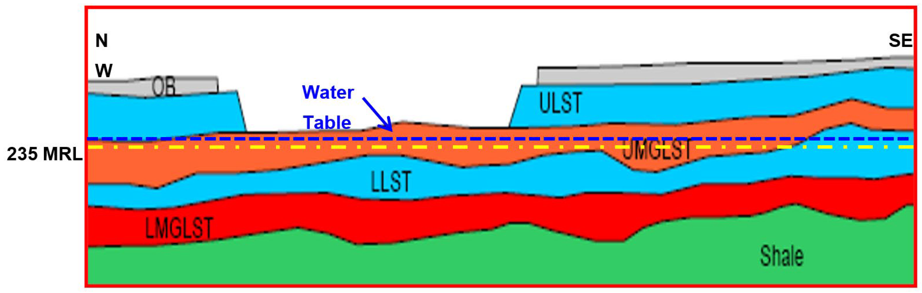
The research was conducted at an Indian limestone mine that serves as a captive limestone mine for a cement mill. The landscape in the case study mine is plain and sloping, with a northeast regional inclination. In the south, the mean elevation is roughly 280 m, whereas, in the north, it is around 240 m above sea level. The mean land slope is 4 m per kilometer. Limestone deposit forms a part of the Chhattisgarh Synclinorium comprising sediments of calcareous, argillaceous, and arenaceous facies represented by the Limestone, shale, and sandstone, respectively. Limestone, magnesian/dolomite limestone, and shale are the principal geological formations found in the area. The beds are mostly horizontal or have a slight incline of 2 to 5 degrees due south. The stratigraphic column of the study limestone mine includes Overburden (OB), Upper Limestone (ULST), Upper MgO Limestone (UMGLST), Lower Limestone (LLST), Lower MgO, and Shale. A typical stratigraphic section of the study limestone mine is presented in Figure 1. The limestone formations run generally northeast-southwest, with modest dips of 2°–3° to the northwest. The deposit has a basic structure, with limestone beds that are practically level and persist at depth.

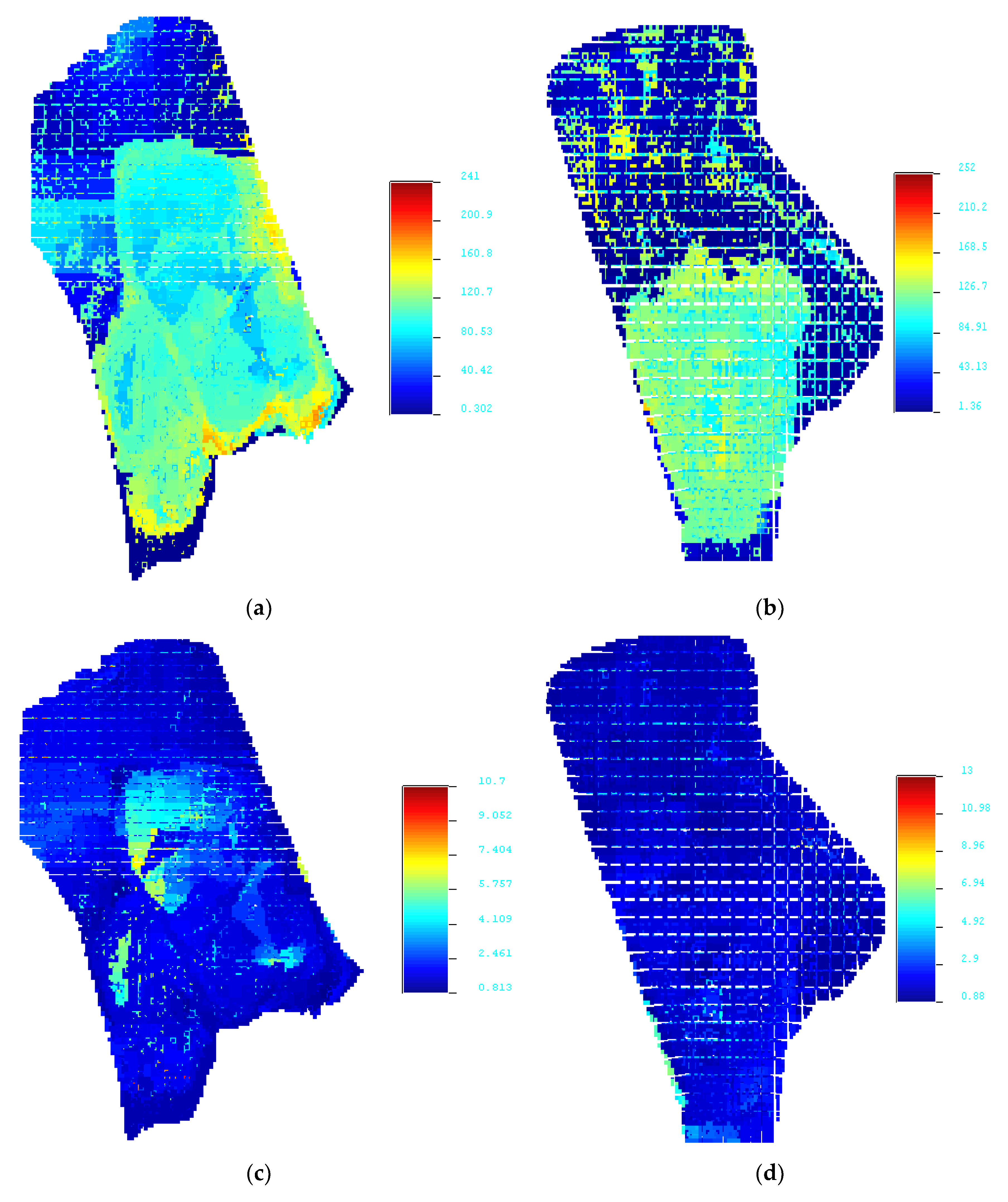
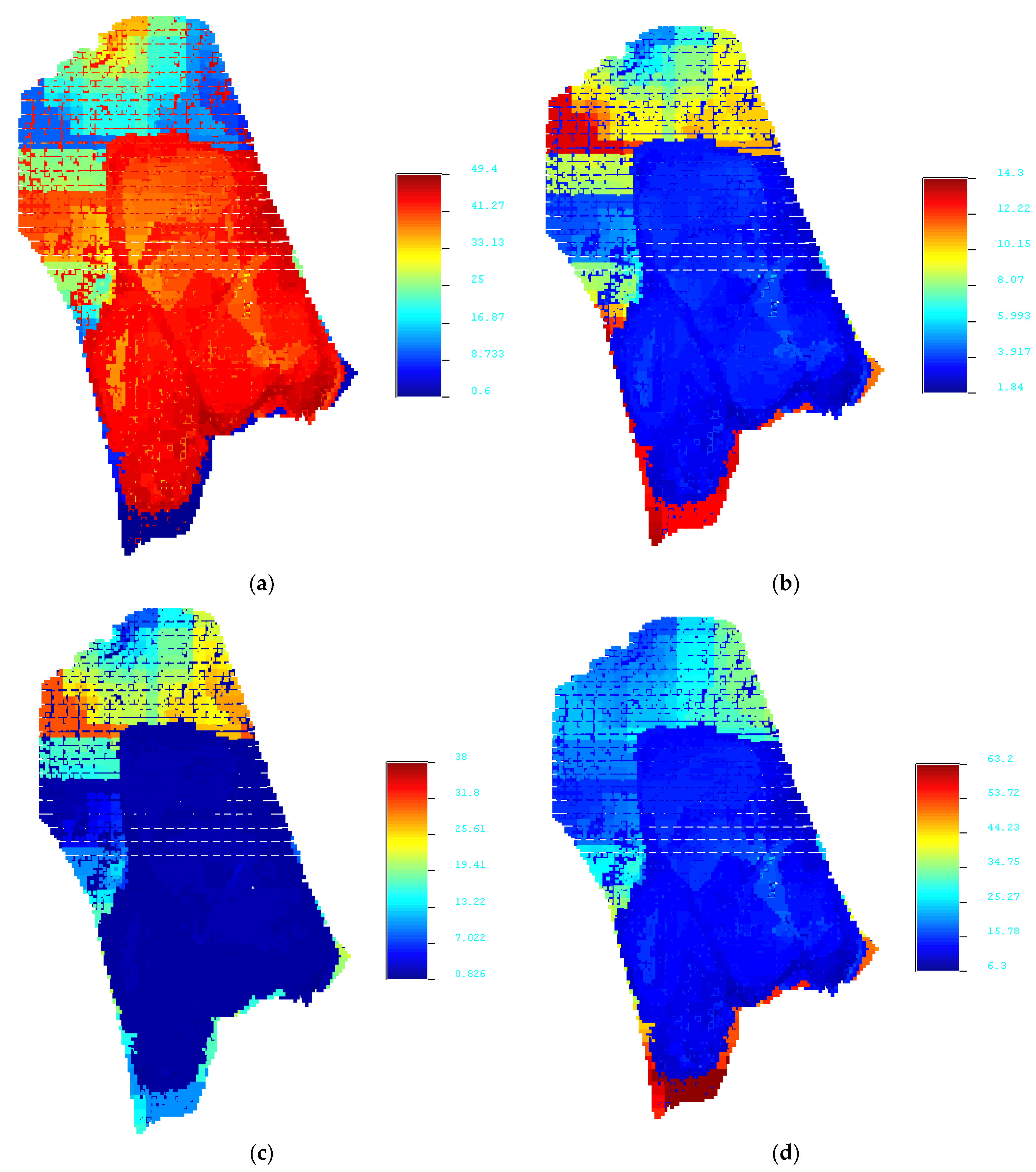
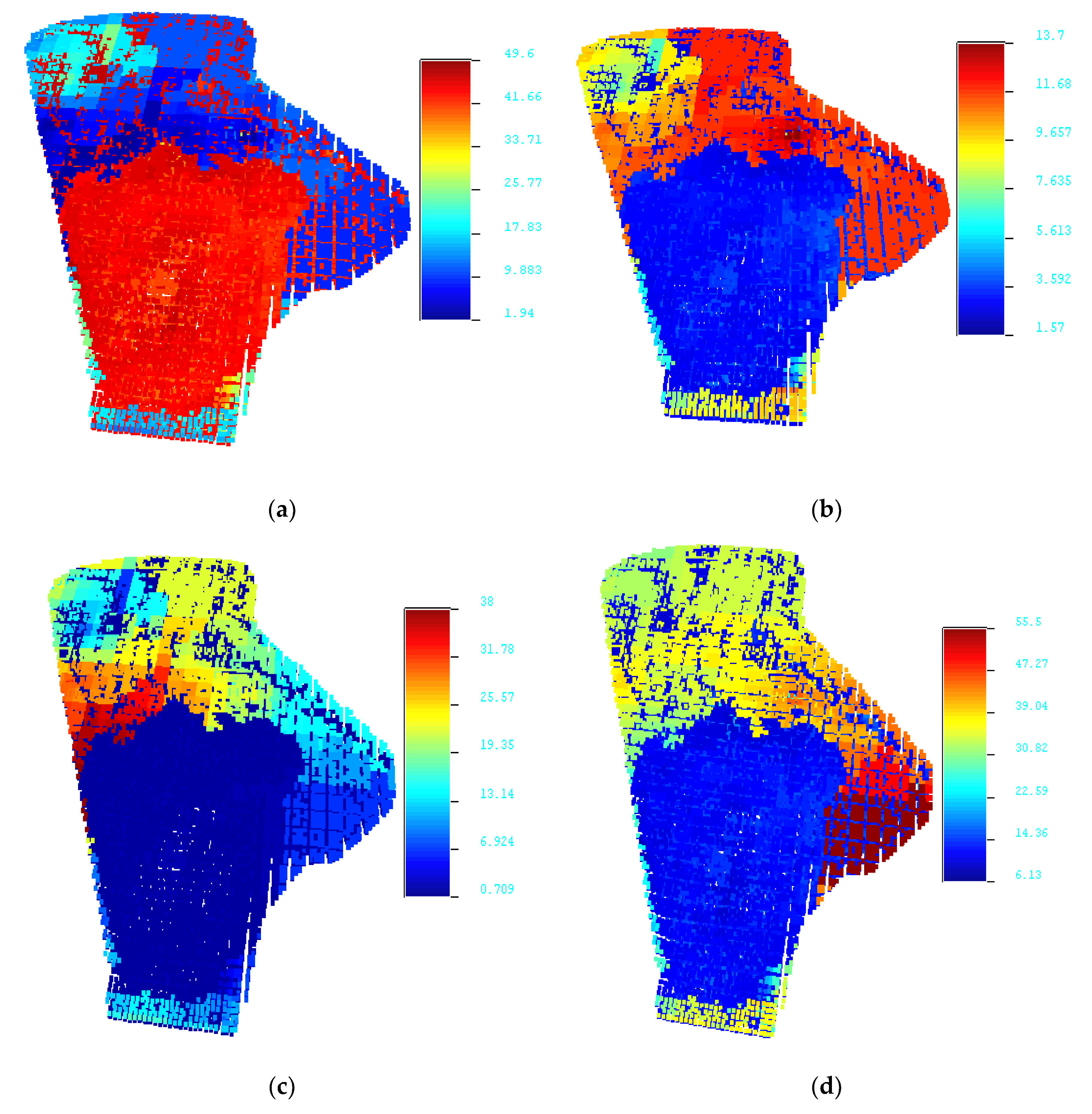
The interstate highway divides the study limestone deposit into two blocks: the north block and the south block. The orebody resource model of the limestone mine was prepared for the parameters like CaO, Al₂O₃, SiO₂, Fe₂O₃, MgO, and specific gravity. The resource models of CaO, Al₂O₃, SiO₂, and Fe₂O₃ are presented in Figure 2 and Figure 3 for both the north and south blocks. 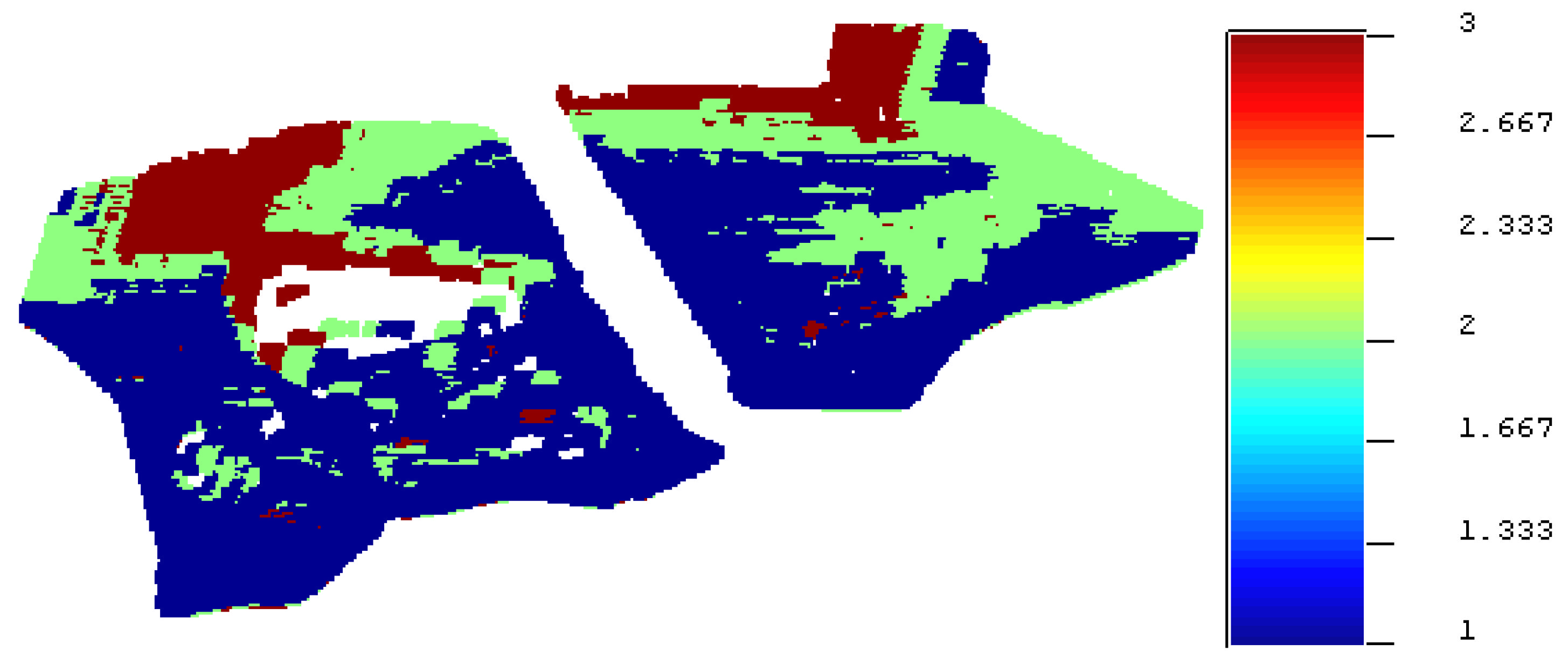The LSF value which is one of the primary parameters was calculated using the CaO, Al₂O₃, SiO₂, and Fe₂O₃ data and Equation (1). 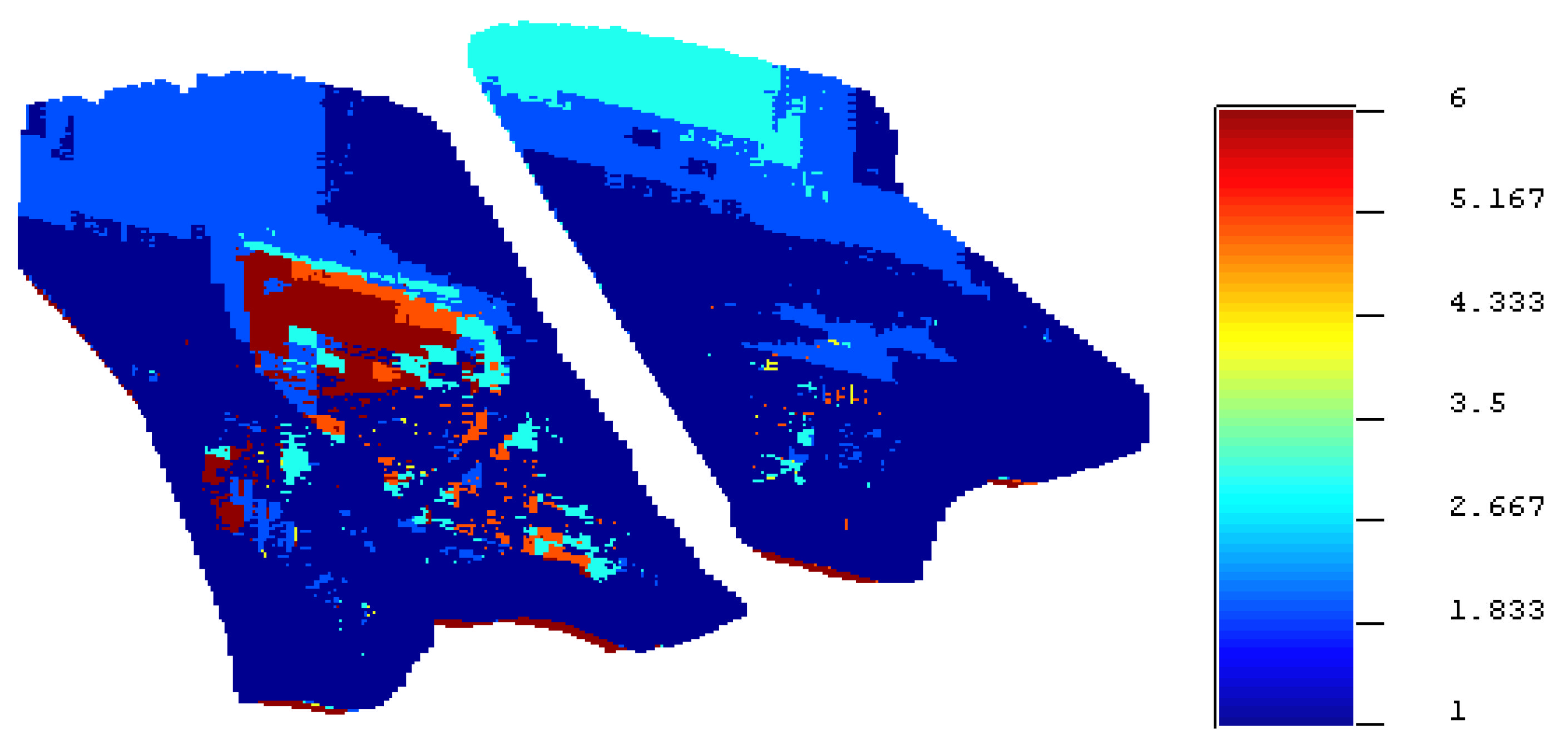The LSF maps and MgO maps for both blocks are presented in Figure 4.

Table 1. The exploratory data analysis of the south block and north block of the case study mine.

	CaO	Al2O3	Fe2O3	SiO2	LSF	MgO
Southern Block
Median	43.31	3.36	1.68	12.67	106.67	2.25
Mean	41.18	3.59	2.37	13.46	106.66	2.85
Variance	43.70	2.34	12.54	33.29	1157.25	2.36
Northern Block
Median	43.23	3.31	1.69	12.75	105.93	2.11
Mean	40.95	3.73	2.69	14.09	106.78	2.47
Variance	65.52	3.81	19.48	49.12	1464.05	1.30

shows the exploratory statistics for all of these factors for both blocks. The median and mean of all of these parameters revealed that the CaO, Al₂O₃, and Fe₂O₃ distributions are approximately Gaussian; however, the MgO and SiO₂ are slightly skewed distributions. For both blocks, this statement remains true. Al₂O₃, CaO, and MgO have relatively low variability, whereas Fe₂O₃ has a comparatively large variability. When these two blocks are compared, it is clear that the northern block has a higher level of variability than the southern block. When the LSF value is determined, it is discovered that it follows a Gaussian distribution.

In this project, optimization models were developed to maximize the discounted net present profit. The objective functions of these two models used the economic value of the individual block as input parameters. The following equation is used to compute the economic value of each block:

$$I_j=RE{V}_j-M{C}_j-MC{A}_j-D{W}_j$$

(17)

where $I_j$ is the economic value of block j, $RE{V}_j$ is the revenue (INR/ton) generated from block j, $M{C}_j$ is mining cost (INR per ton) of the block j, $MC{A}_j$ is the mining cost adjustment factor of block j, $D{W}_j$ is the dewatering cost of block j. The $RE{V}_j$, $M{C}_j$, $MC{A}_j$, and $D{W}_j$ of the block, j is calculated as:

$$RE{V}_j=\left\{\begin{array}{c}\mathrm{INR} 100 \mathrm{if} L{S}_j<60\\ \mathrm{INR} 170 \mathrm{if} L{S}_j\ge 90\\ \mathrm{INR} 130 \mathrm{If} 90>L{S}_j\ge 60\end{array}\right.$$

$M{C}_j$ of block j including royalties, taxes and all cost parameters are INR 170.

$MC{A}_j$ of a block, j per bench (9 m) below 235 mRL is INR 5.

$D{W}_j$ of a block, j per bench (9 m) below 235 mRL is INR 3.

After calculating the economic value of the block, the data are used for production planning. The present total number of blocks in the limestone mine’s north and south blocks is 216,193, and 273,407, respectively. There are 489,600 blocks in total in the deposit. Because the no. of blocks in the deposit is so large, no solver can manage the production scheduling problem optimally even after solving it period after period. In this study, the blocks are first mapped into clusters, as indicated in the solution approach, to decrease the quantity of decision factors. Although the sub-problem formulation reduces the computation time of the original formulation, the sub-problem still has a significant amount of computational burden due to resource constraints. To further reduce the processing complexity of the production schedule for the limestone mine, several decision factors (such as a group of mining blocks) are consolidated and mapped to a single decision variable. To group the choice variables, the k-means clustering algorithm [26] was applied. This effort resolves the constraint k-means clustering problem as opposed to traditional k-means clustering, which resolves the problem with no restrictions. The requirement, in this case, is that the individuals who make up the group of choice variables get into direct range of one another. The adjacent factor was assessed using the adjacency matrix. Once the number of clusters was established and the cluster centers were computed, the clusters were formed. The centers of the clusters were then determined to be the deciding factors. After being mapped, the cluster centers are employed as new decision variables in the production scheduling issue. All block members in a single cluster were made to make the same decision; for example, if a particular cluster is extracted in period t, all blocks mapped in that cluster are also extracted in period t. The number of choice factors is greatly reduced with this method. The fundamental tree algorithm suggested by Ramazan [27] was applied in this study to cluster the data. There are 15,796 and 12,289 clusters selected for the southern and northern blocks, respectively. As a result, the deposits total number of clusters is 28,085. Then, these clusters are used for production scheduling. When the statistics of the clustered data are compared to the statistics of the actual resource model, no significant differences are found. Among several clustering algorithms, K-means is the fastest centroid-based technique. The K-means clustering technique assigns each mining block to one of the $K$ predefined classes or groups through an iterative process. K-means clustering returns the cluster centers, or centroids, which correspond to the average value of each cluster’s block attributes as an associated output. The mass of the clusters and the individual parameters were calculated using the following equations:

$$C_j={\displaystyle \sum _{i=1}^s{c}_i} j=1,2,\dots ,J$$

(18)

$$C\_L{S}_j=\frac{{\displaystyle \sum _{i=1}^s{c}_i\ast L{S}_i}}{{\displaystyle \sum _{i=1}^s{c}_i}} j=1,2,\dots ,J$$

(19)

$$C\_m{g}_j=\frac{{\displaystyle \sum _{i=1}^s{c}_i\ast m{g}_i}}{{\displaystyle \sum _{i=1}^s{c}_i}} j=1,2,\dots ,J$$

(20)

where $C_j$, $C\_L{S}_j$, and $C\_m{g}_j$ are mass, lime saturation factor, and MgO, respectively, for the cluster j and, s is the number of decision variables mapped to the cluster j. After mapping the cluster centers, they are used as new decision variables for the production scheduling problem. The slope constraints are prepared for the set of decision variables.

6. Results and Discussion

The limestone deposit is divided into two blocks by the highway, i.e., the northern block and the southern block. The separate ultimate pit and production planning were performed by a mine in their long-range plant. The mining lease boundary, ultimate pit limit for both northern and southern blocks, and current working pits for both northern and southern blocks according to the Cement plant. Production planning was done using clustered data from a northern block and a southern block. The boundaries for LSF were 103 and 107, which correspond to the cement plant’s necessary LSF value. For the cement plant, the maximum allowed limit for MgO in limestone was 2.5%. The plant’s yearly limestone need is 6.31 million tons. Production planning of the limestone mine was done for five years in this study. As a result, for both difficulties, the maximum production target from the study mine per period was taken into account. A lower bound limit of the output objective was also defined to reduce the idle time of mining equipment, and that value is 30 million tons. For Model 2, it changes upper limit is 21.50 million tons and the lower limit is 20 million tons. The branch and cut approach was used to tackle the integer and mixed integer programming problems.

7. Results and Discussion of Model 1

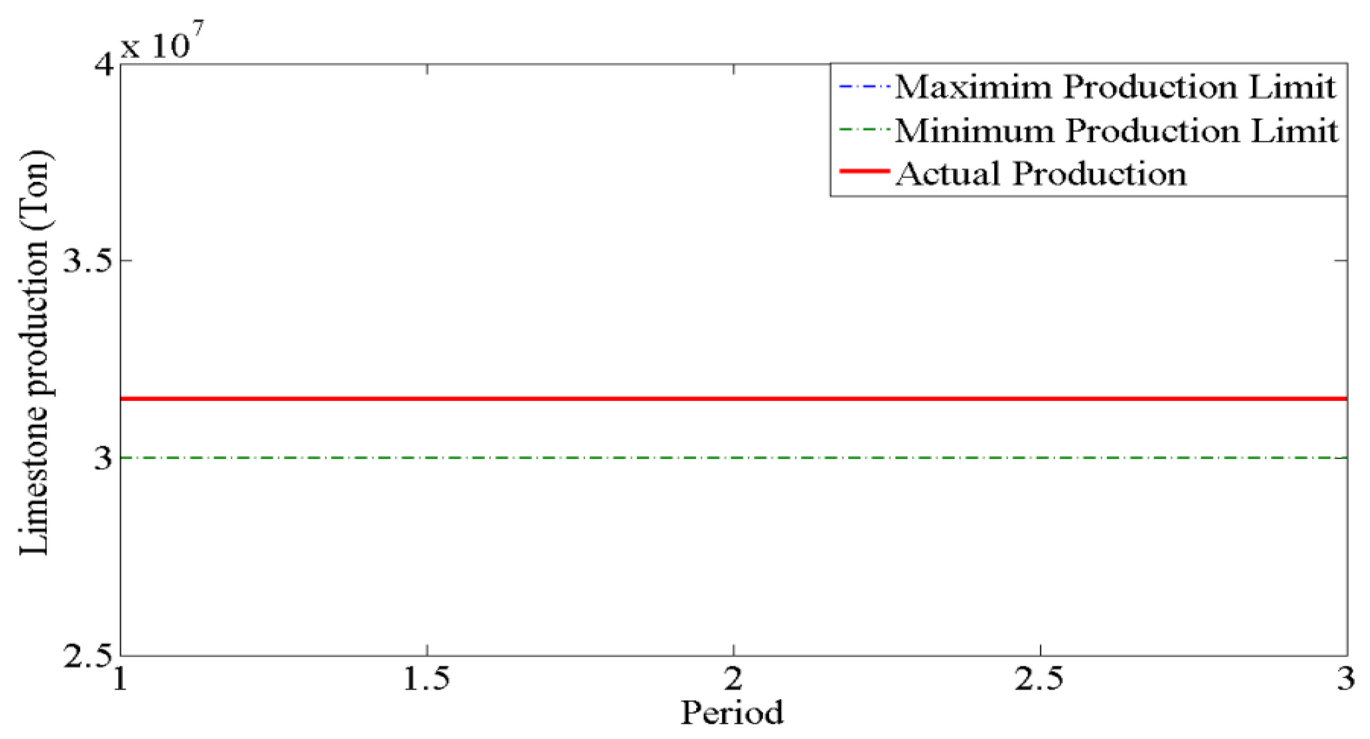
The purpose of this model is to maximize profit while determining the final pit limit and the life of the limestone mine. No additional limestone from other sources was used in this model to meet the cement plant’s requirements. As a result, the model’s results show that the case study limestone mine seems to have the potential to be the cement plant’s single source of the desired quantity and quality of limestone. After applying the branch and cut method to this model, it was determined that it can create feasible solutions up to period 3, indicating that the mine can only serve as the cement plant’s only source of limestone for 15 years. Figure 5 depicts the production of limestone for three years, and shows that limestone output reaches the highest permissible limit, which is 31.55 million tons, which is the study mine’s target production. 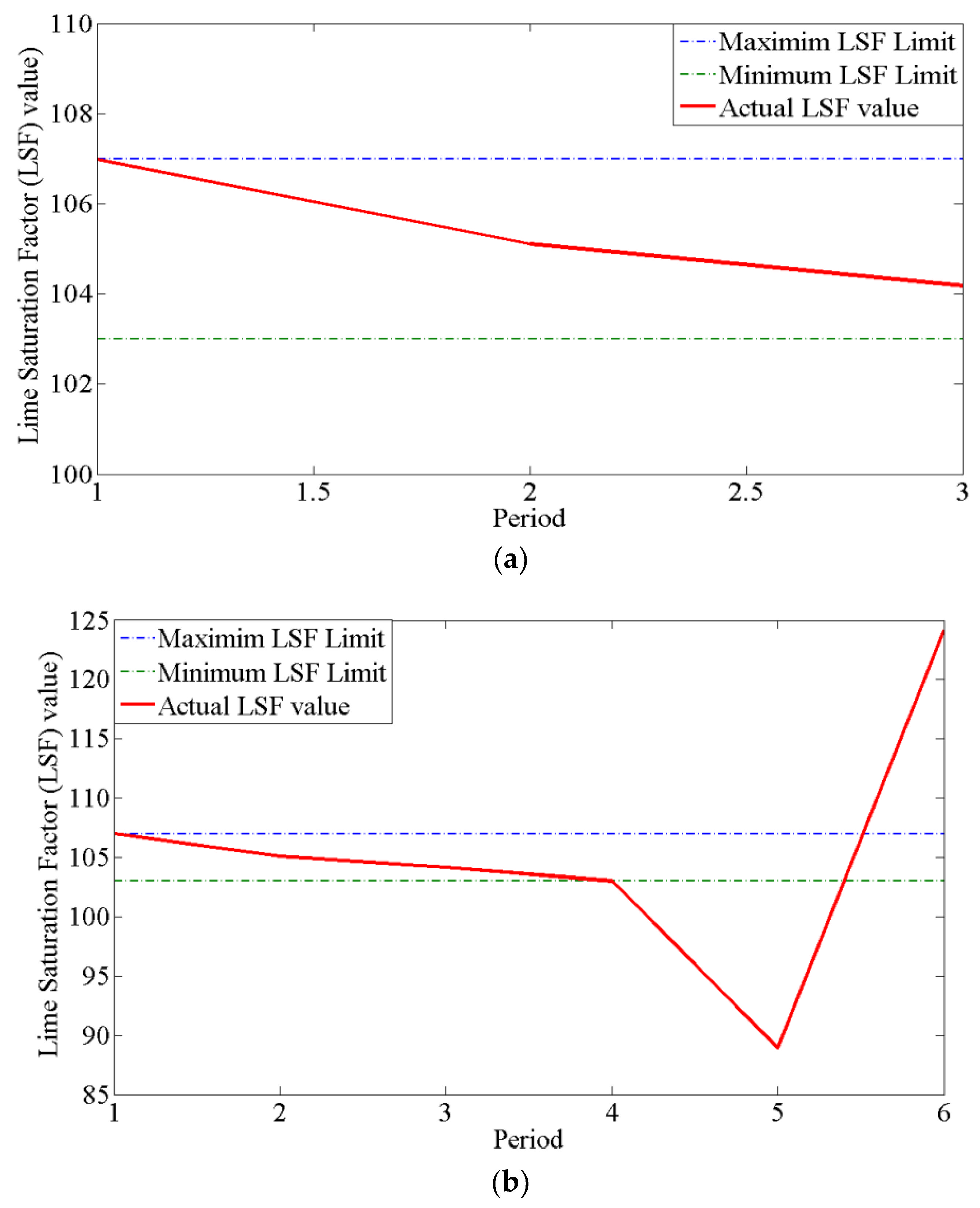Figure 6a,b show the average LSF values for these three and six periods. The average LSF values are gradually dropping from period one to period three as shown in the graph. Because profit is a function of LSF, greater LSF values ensure higher profit. 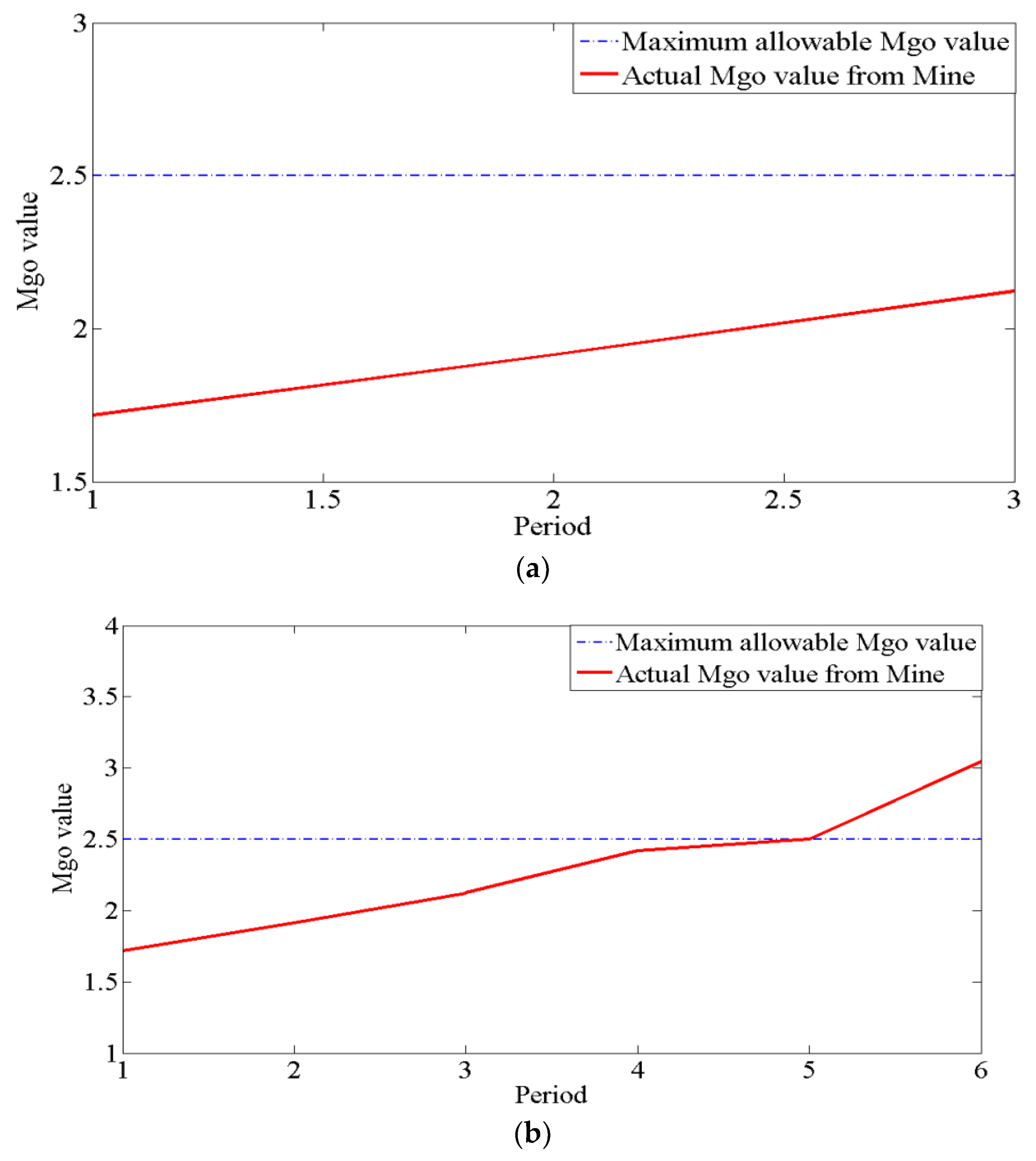Figure 7a,b show the average MgO values for these periods three and six. The average MgO values are growing, as seen in the graph, although they are still within acceptable limits up to the third period. Figure 8 depicts the production schedule. To check whether the ultimate pit can be extended beyond the third period if the constraints are eliminated, model 1 was solved using the blocks left over after period three and relaxing the constraints. The ultimate pit is considered until the objective function value is positive which ensures profit from the deposit. First production limit constraints were eliminated, then LSF constraints, and finally, the MgO constraints. This way the pit can be extended up to the sixth period. The limestone productions, LSF, MgO, and undiscounted cash flow up to six periods are represented in

Table 2. Production scheduling results from Model 1.

Period	LSF	MgO (%)	Production (Million Ton)	Undiscounted Cash Flow (Million INR)
1	106.99	1.72	31.5	1940
2	105.10	1.92	31.5	1960
3	104.18	2.12	31.5	1960
4	103.07	2.42	2.35	135
5	88.89	2.45	18.54	670
6	124.16	3.04	242	7690
Total			357.39	14,355

. It was viewed from the Table that the productions violated marginally the lower bounds in period five; however, there is a substantial deviation in the fourth and sixth periods. It was viewed from the results that the LSF value touches the lower bound in the fourth period; however, after the fourth period, these values are far from the bound (one far below and one far above). It was also observed from the results the MgO value is within the range in the fourth and fifth periods; however, after the sixth periods, the MgO value is higher than the maximum allowable value. The total undiscounted profit from the limestone deposit using this model is INR 1.44 × 10¹⁰. The total amount of limestone present within the relaxed solution of the ultimate pit is 357 million tons. This is a crucial observation that when applying the economic parameters as an objective function in production planning, more profit can be generated by extracting less amount of materials. The relaxed model’s ultimate pit is represented in Figure 9.

8. Results and Discussion of Model 2

This model is using the same objective function as Model 1. The main difference between Model 1 and this model is that here so the plant management has the flexibility to bring limestone from the nearby mine. The cement factory management has chosen to bring 2 million tons of limestone per year from a nearby mine and blend it with the limestone from the study mine to solve this problem. As a result, 10 million tons of limestone will be transported per period from another mine. This model aids in determining the limestone feeding grades that will be brought in from other mines. Moreover, by maximizing the net discounted cash flow, the model assists in optimizing the extraction sequence and the ultimate pit limit of the study limestone mine. As a result, this model assists cement plant management in determining how long the study limestone mine will be able to feed the cement plant if 2 million tons of limestone are brought in from outside. 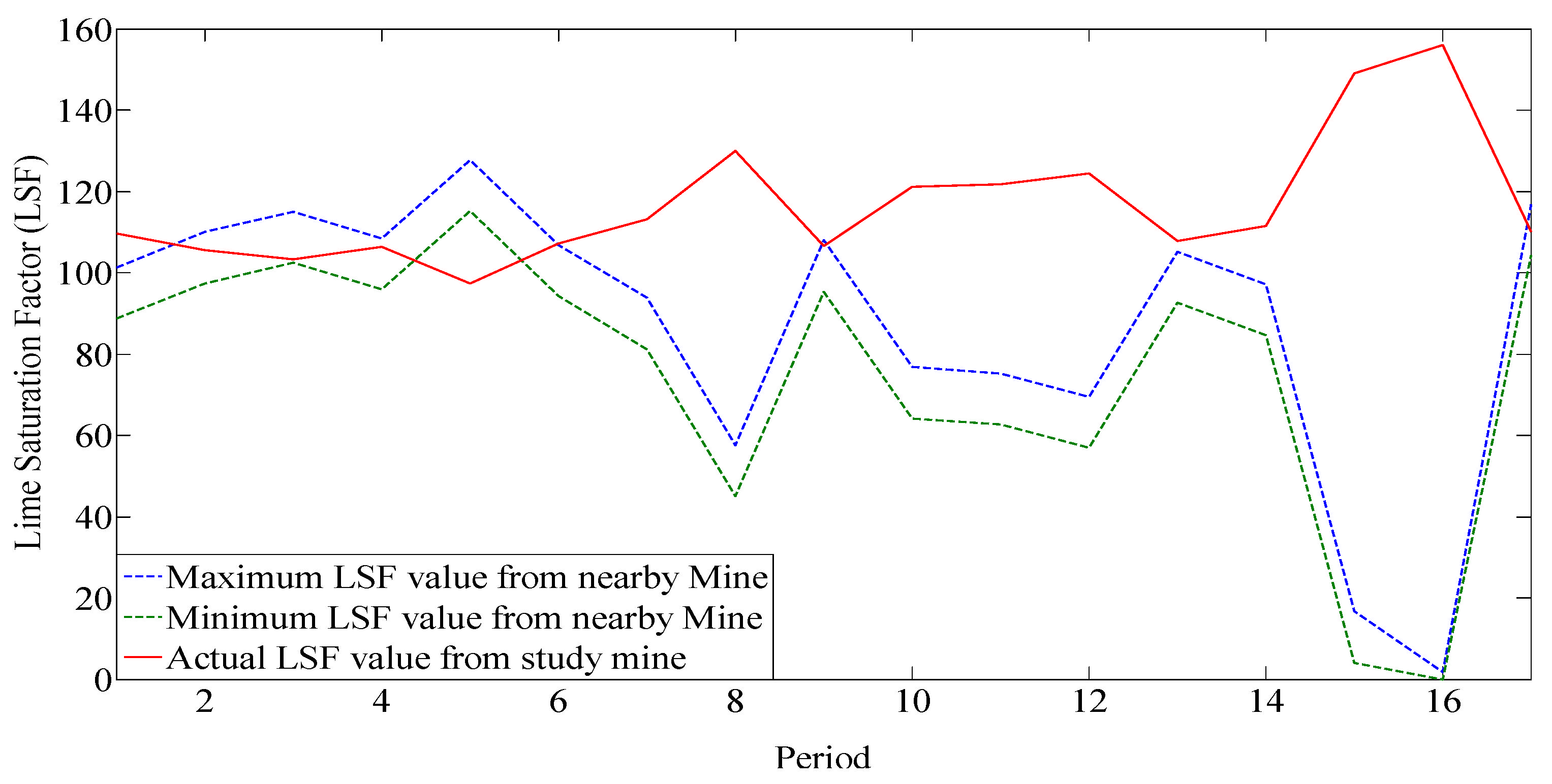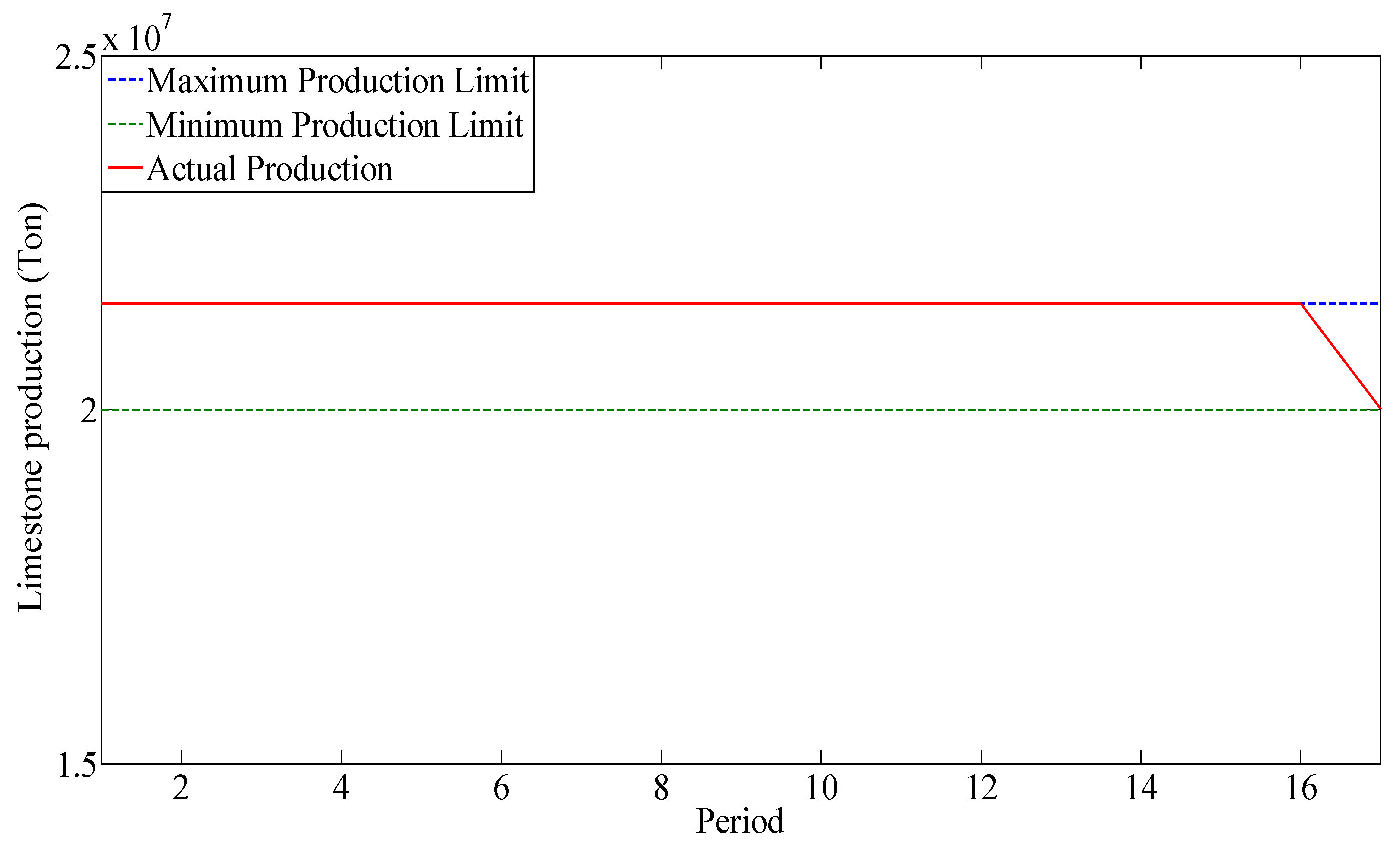If the 10 million tons of limestone can be brought from a nearby mine during each period (one period here is five years), the study mine can serve for 17 periods, or 85 years, according to the Branch and cut algorithm. When compared to Model 1, where mine life can be as long as 15 years, this is an interesting observation. Figure 10 shows the production of limestone through time over 17 periods and shows that limestone output corresponds to the maximum production limit for the first 16 periods, while the 17th period barely touches the lower limit. The reduced output in the last period is because there are insufficient materials in the pit to extract at that time; yet, that figure is within the required production limit. 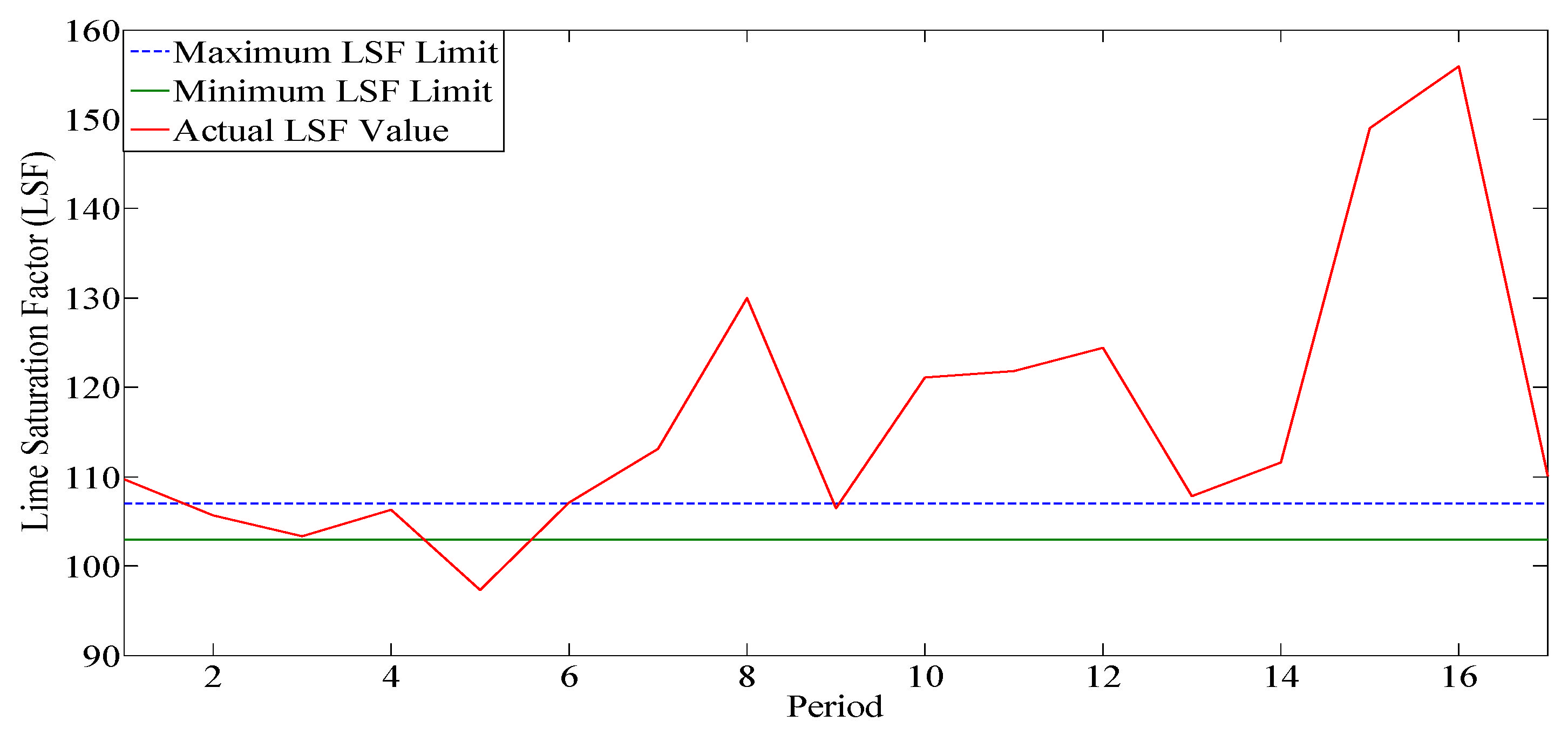Figure 11 shows the average LSF values from the study mine during 17 periods. The LSF values fluctuate quite close to the intended range of up to seven periods, according to the figure; however, after eight periods, the value is over the maximum target LSF value. Figure 12 shows the maximum and minimum LSF values for the limestone brought from the other source for each of the 17 periods. If the limestone supplied from the other source falls within the range represented in Figure 12, a continuous supply of the adequate quantity and quality of limestone to the cement plant is achievable. 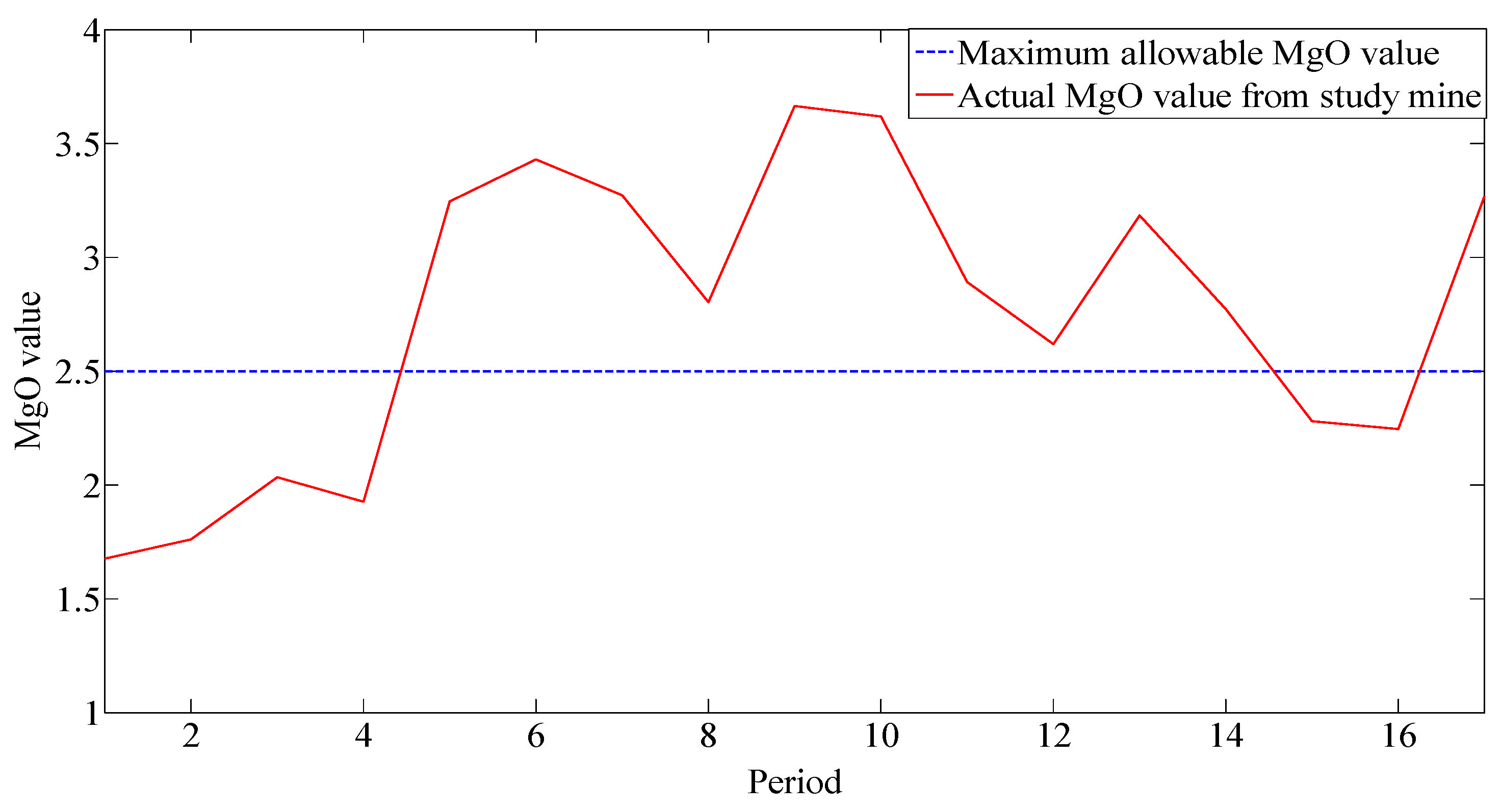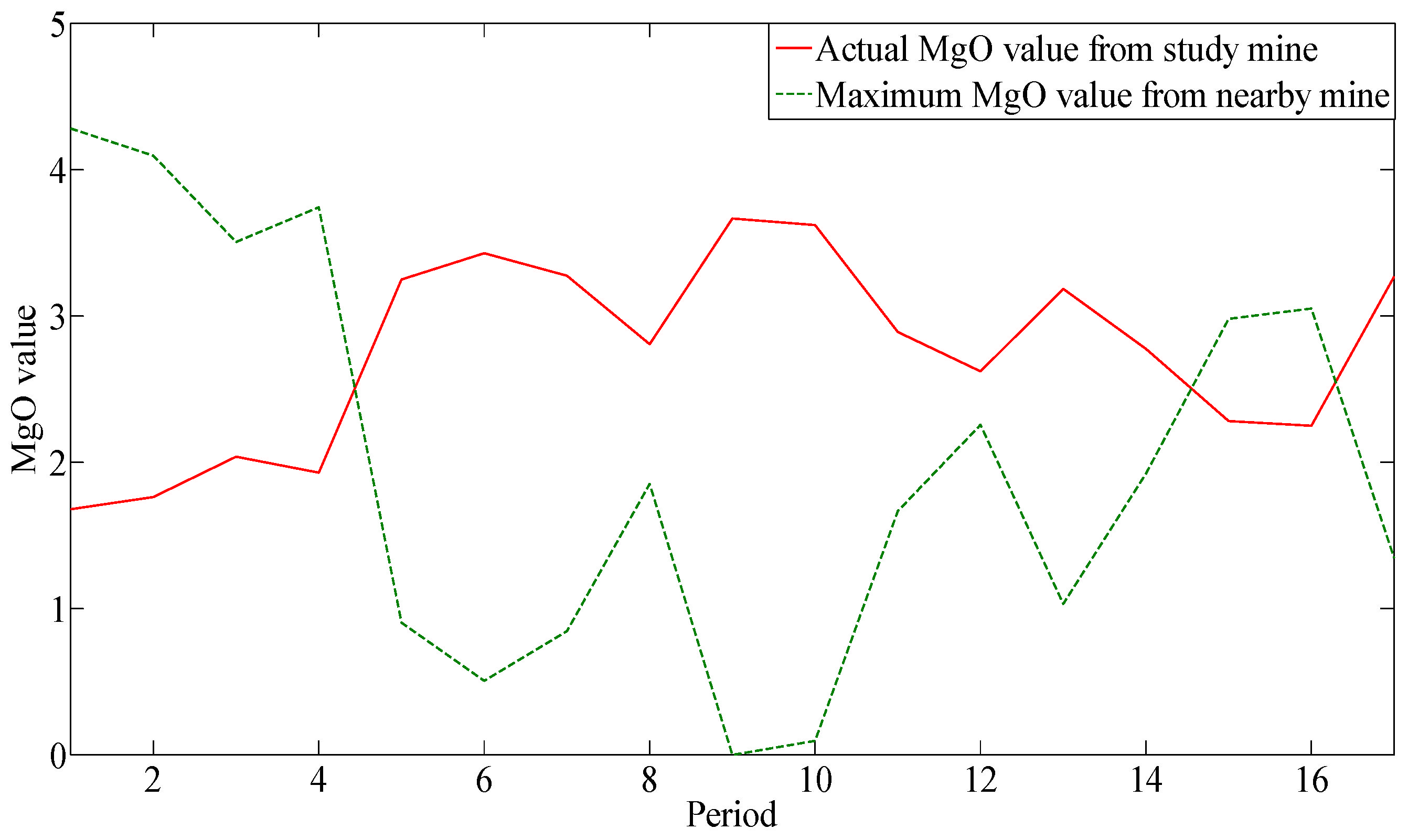Figure 13 shows the MgO values for these 17 periods. The average MgO values are within the limit up to the third period, then show an increasing trend, and finally a decreasing trend. For the first three periods, the study mine itself is supplying the limestone within the MgO bound, so there is nothing to worry much for the management about the MgO problem; however, after third period, management needs to be careful in selecting the limestone from the nearby mine for blending purpose. Figure 14 shows the maximum permitted MgO values for limestone from a nearby mine for 17 different periods. As can be seen in the figure, the limestone provided from the nearby mine can initially have a high MgO value; but, for later periods, suitable consideration of limestone from the nearby mine is essential. It is observed from the figure that the average MgO values are showing decreasing trends; for most of these periods, the Rawan mine is not able to supply the limestone within the allowable MgO value. The maximum allowable values of the MgO for the limestone from the nearby mine for 17 periods are presented in Figure. It is observed from the Figure 13, as expected, initially, the limestone that will be supplied from the nearby mine should have a very MgO value. The undiscounted cash flow is also calculated for this problem (

Table 3. Production scheduling results of Model 2.

Period	LSFR	LSFmax	LSFmin	MgOR(%)	MgOmax(%)	Cash Flow (Million INR)	Production from Study Mine (Million Ton)
1	109.66	101.29	88.70	1.67	4.28	1340	21.50
2	105.63	109.95	97.35	1.76	4.09	1320	21.50
3	103.29	114.99	102.39	2.03	3.50	1340	21.50
4	106.33	108.45	95.85	1.92	3.74	1370	21.50
5	97.33	127.79	115.19	3.24	0.90	1170	21.50
6	107.11	106.76	94.16	3.43	0.50	966	21.50
7	113.15	93.80	81.20	3.27	0.85	873	21.50
8	130.01	57.54	44.94	2.80	1.85	813	21.50
9	106.49	107.95	95.35	3.66	0	722	21.52
10	121.08	76.74	64.14	3.62	0.09	669	21.50
11	121.77	75.25	62.65	2.89	1.66	616	21.50
12	124.43	69.53	56.93	2.62	2.25	582	21.50
13	107.83	105.22	92.62	3.18	1.03	604	21.50
14	111.56	97.21	84.61	2.77	1.92	597	21.50
15	149.02	16.70	4.10	2.28	2.98	648	21.50
16	155.96	1.77	0	2.25	3.05	518	21.50
17	110	116.86	104.26	3.27	1.34	123	20.00
Total						14.271	364.02

* LSF_R = Study mine LSF value; LSF_max = Maximum LSF value from the nearby mine; LSF_min = Minimum LSF value from the nearby mine; MgO_R = Study mine MgO value; MgO_max = Maximum MgO value from the nearby mine.

). The total undiscounted profit generated using this model is INR 1.43 ×10¹⁰, which is almost similar to Model 1. However, Model 1, cannot provide any production schedule for the deposit after the third period. The total amount of limestone in the ultimate pit is 364 million tons, which is significantly greater than in Model 1. There for, the size of the ultimate pit for Model 2 will be more than that of Model 1. The production schedule and the ultimate pit of the model are also presented in Figure 15.

9. Comparisons of Models

A comparative study of two models (Model 1 and Model 2) was performed to see the effectiveness of the study. First, the amount of ore, waste, total materials within the ultimate pits, stripping ratio, and undiscounted cash flow were calculated and presented in

Table 4. Amount of waste, ore, total materials, and stripping ratio of an ultimate pit of the deposit for Model 1 and Model 2.

Model Number	Amount of Waste (Million Ton)	Amount of Ore (Million Ton)	Total Material (Million Ton)	Stripping Ratio	Undiscounted Cash Flow (Million INR)
1	6.99	350.4	357.39	2.00 × 10−2	14355
2	13.5	350.52	364.02	3.85 × 10−2	14271

. For determining the ore and waste, we used the same cut-off value that the study mine uses presently, i.e., 60 LSF. The results demonstrated that Model 2 produces more amount of waste compared to Model 1. The reason is that the limestone that is treated as waste by the plant management, could be sent to the cement plant by blending with high-grade limestone from other sources. Results also demonstrated that both models produce the almost same amount of ore within the ultimate pit. The stripping ratio is relatively small in Model 1 because it produces a lesser amount of waste materials. The undiscounted cash flow is almost the same for both these models, however, it is noted that Model 1 can’t produce the production schedule therefore, a true comparison of the discounted cash flow can’t be possible.

Furthermore, a comparison with the existing optimization model [19] of the study mine was performed with Model 2 which provides a production schedule. In their existing optimization models, the plant management was performing almost the same problem as discussed in this paper, with different objective functions. The current model focuses on maximizing the exploitation of limestone with an LSF value of 60 to 90 by bringing in the same amount of limestone from other sources (2 million tons per year). All the constraints and decision variables are exactly same as Model 2. The optimization formulation and detailed results of the existing method can be found [19]. The amount of ore, waste, total materials within the ultimate pits, stripping ratio, and undiscounted cash flow were calculated and presented in

Table 5. Amount of waste, ore, total materials, and stripping ratio of an ultimate pit of the deposit using the proposed model (Model 2) and existing model [19].

Model Number	Amount of Waste (Million Ton)	Amount of Ore (Million Ton)	Total Material (Million Ton)	Stripping Ratio	Undiscounted Cash Flow (Million INR)
Existing model	19.9	344.56	364.46	5.76 × 10−2	13,987
Proposed model	13.5	350.52	364.02	3.85 × 10−2	14,271

. The results reveal the fact that when economic parameters are used as an objective function (the proposed model in this paper), there is a possibility of extracting less amount of waste materials when compared with the existing method. When the stripping ratios were compared, it was found that the suggested approach has a substantially lower stripping ratio than the existing method, confirming that the economic factors in the objective function aid to reduce the amount of waste extraction per ton of ore removed. The undiscounted cash flow results also show that a proposed model produces more cash flow than the existing model. The reason is that in the proposed model, the higher quality materials are scheduled in the initial period to generate more cash flow; however, the existing model tries to use the lower quality limestone at the initial stage. So, when the model reaches the final stage i.e., close to the end of periods, there are plenty of higher quality materials left but due to the geotechnical constraints, they were not extracted.

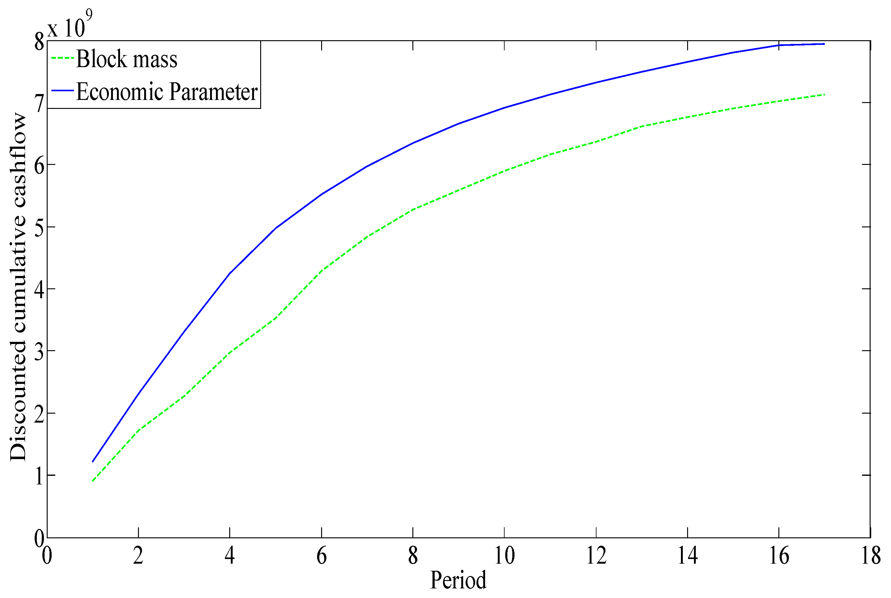
The existing model’s undiscounted cumulative cash flow and the proposed model’s undiscounted cumulative cash flow were compared, and the results showed that the proposed model can generate 2% more cash flow than the existing model. The undiscounted cash flow, on the other hand, does not account for the time worth of money. When compared to undiscounted cash flow, the outcome can be misleading. As a result, the discounted cash flow for the existing model and the proposed model was calculated and shown in Figure 16. The discounted cash flow calculation employs a 10% discount rate. The results show that the new model generated around 10% greater cash flow than the existing model. As a result, if economic parameters are available, it is always preferable to execute production planning and ultimate pit limit calculation using those values.

10. Conclusions and Future Scope

From this study, the following observations were made: limestone mines alone can be serve the cement plant for 15 years. If the economic parameter is used as an objective function, the mine generates more profit. When 2 million tons of materials are supplied from other sources, the life of the mine is increased up to 85 years. Long-term planning for the limestone mine was carried out in this article. The ultimate pit limit, as well as production scheduling, were both completed. This study’s main goal was to determine how well the study mine could provide a cement plant with the appropriate quantity and quality of limestone while also maximizing the deposit’s net profit. According to the results, the limestone quarry undergoing study can consistently feed the cement plant for 15 years. The project’s second goal was to determine how long the study mine could last if more limestone could be obtained from other sources. The results showed that by bringing 2 million tons of limestone from another source to blend with the limestone in the study mine, the mine’s life might be extended to 85 years. When compared to the existing model [19], the quantity of limestone in the ultimate pit in this model is significantly higher; however, the undiscounted cash flow is nearly identical. It was discovered that when compared to the existing system, the proposed method yields greater discounted cash flow (10% more). According to the research, it was found that the limestone from the nearby mine that would initially be supplied might have a high MgO value; however, for the later periods, careful selection of the limestone from the nearby mine is required for blending. The computed quality criteria for the limestone provided from other sources, such as the LSF bound and maximum MgO values, assist management in finding suitable quality materials from other nearby mines to reach the desired grade after mixing these materials. The proposed method’s fundamental flaw is that it ignores the quality of information from other sources. Understanding the fundamental complexities of developing a comprehensive model, however, in the future, not only the qualitative composition, but also the quantitative capabilities of the nearby mine are taken into account. Incorporating the quality and quantity criteria of the limestone from the other source assures that the desired quality and quantity of materials will be available from that source, which will be investigated further in the future.