Article

Affine Term Structure Models: Applications in Portfolio Optimization and Change Point Detection

by
Konstantinos Bisiotis
1,
Stelios Psarakis
2,* and
Athanasios N. Yannacopoulos
3
1
Department of Statistics and Department of Accounting and Finance, Athens University of Economics and Business, Patission 76, 104 34 Athens, Greece
2
Department of Statistics and Laboratory of Statistical Methodology, Athens University of Economics and Business, Patission 76, 104 34 Athens, Greece
3
Stochastic Modeling and Applications Laboratory, Department of Statistics, Athens University of Economics and Business, Patission 76, 104 34 Athens, Greece
*
Author to whom correspondence should be addressed.
Mathematics 2022, 10(21), 4094; https://doi.org/10.3390/math10214094
Submission received: 12 October 2022 / Revised: 25 October 2022 / Accepted: 26 October 2022 / Published: 3 November 2022

Abstract

:
Affine term structure models are widely used for studying the relationship between yields on assets of different maturities. However, it can be a helpful tool for the construction of fixed-income portfolios. The monitoring of these bond portfolios is of great importance for the investor. The purpose of this work is twofold. Firstly, we construct and optimize fixed-income portfolios using Markowitz’s portfolio approach to a multifactor Gaussian affine term structure model (ATSM) under no-arbitrage conditions estimated with the minimum chi square estimation method. The fixed-income portfolios based on the term structure model are compared with some benchmark portfolio strategies, and our findings show that our proposed approach performs well under the risk–return tradeoff. Secondly, we propose control chart procedures for monitoring the optimal weights of government bond portfolios in order to detect possible changes. The results indicate that control chart procedures can be useful in the detection of changes in the optimal asset allocation of fixed income portfolios.
MSC:
91G10; 91G30; 62P30

1. Introduction

Dynamic term structure models play an important role in fixed-income asset pricing and strategic asset allocation. However, the connection between dynamic factor models and portfolio optimization has been explored only in recent years. The literature is mainly focused on the construction and performance of equity portfolios under the mean variance (MV) approach (see for example [1,2]). Ref. [3] examined the the validity of the expectation hypothesis (EH) of the term structure of U.S. repo rates and the profitability of portfolios of bonds that exploit deviations from the EH. Ref. [4] investigated the MV analysis immunization to real yield curve fluctuations under the Vasicek term structure model. Ref. [5] using the Vasicek term structure model examined the optimal portfolio choice under inflation risk. Refs. [6,7,8] constructed optimal portfolios generated from various Nelson–Siegel term structure models. Ref. [9] mentioned that if we can estimate expected bond returns and their variance–covariance matrix, the portfolio optimization procedure is similar to that of equity portfolios.
The majority of the literature about dynamic factor models and bond portfolios is focused on the dynamic Nelson–Siegel model. In addition, the application of control chart procedures is referred mainly to stock portfolios. Our research deals with a different class of factor models, the Gaussian affine term structure model (ATSM) with the minimum chi square estimator, and extends the application of control chart procedures to government bond portfolios. Minimum chi-square estimation (MCSE) avoids many of the numerical problems associated with the maximum likelihood estimation (MLE) for the affine term structure models and ensures the finding of global maximum solutions ([10].) Following the work of [8], we obtain closed-form solutions for the expected bond returns and the covariance matrix of bond returns but for a different class of dynamic factor models. The purpose of this work is, firstly, the construction of an MV and global minimum variance (GMV) portfolio that consists of government bonds via a no-arbitrage ATSM and secondly to apply exponentially weighted moving average (EWMA) control charts for monitoring the optimal portfolio weights. For the covariance of the proposed control statistics, we propose an iterative procedure.
We mention that in our case, the asset returns, which are the bond expected returns, due to their structure exhibit autocorrelation, and appropriate control charts are constructed. The expected return and variance of bond yields are estimated from the distribution of a dynamic term structure model. The results indicate that the proposed technique for obtaining bond portfolios could be a good alternative to other existing methods, and we determine the appropriate monitoring procedure for the fixed-income portfolio.
Government bonds issued by national governments are generally considered low-risk investments in comparison with stocks. Bonds are usually less volatile than stocks, and many investors include bonds in their portfolio as a source of diversification so as to reduce potential losses and overall portfolio risk. Investing in sovereign bonds, especially in times of economic turmoil, could be a safer choice for individual and institutional investors such as pension funds. The investor at every time is interested in the optimal portfolio weights, and structural breaks may cause changes that may have economic effects. The portfolio investor needs to detect these breaks as soon as possible, since they may alter the optimal portfolio composition. The presence of structural breaks can influence the estimation of the portfolio parameters and affects the forecasting procedures. The investor decides every time period about the optimal wealth allocation. As a result, he needs to know whether the optimal portfolio allocation in the previous time period can be still considered now as the optimal. If the current portfolio position is not the optimal, then the investor could face wealth losses. The new information about bond expected returns arrives sequentially, and the optimal portfolio weights should be monitored in a sequential manner. In order to do this, we apply statistical process control (SPC) methods, specially control charts, for deciding whether the optimal portfolio weights of the last period are still optimal in the current period.
In Section 2, we present the related literature, and in Section 3, we describe our data set. Next, in Section 4, we estimate the term structure model, the one-period ahead expected returns and the variance of the bond yields for a specified out-of-sample period. In Section 5, we present the framework and the results for the fixed-income portfolio optimization. Section 6 deals with the application of control charts to optimal weights of a global minimum variance portfolio (GMVP). Section 7 and Section 8 present the results of a simulation study and an empirical example, respectively. Finally, in Section 9, we present the conclusion of this work and our contribution.

2. Related Literature

According to [11], since the processes that affect both bond price and bond return are non-ergodic, the traditional statistical techniques cannot be used to directly model the expected return and volatility of bond yields. Refs. [12,13] proposed the use of the one-factor [14] model for the yield curve for the mean variance bond portfolios optimization. In contrast, our analysis refers to the category of multifactor dynamic term structure model exploiting the forecasting benefits they have in comparison to one-factor models. Ref. [8] are focused on Nelson–Siegel models, the Gaussian dynamic term structure model of [15] and the no-arbitrage representation of a dynamic Nelson–Siegel model of [16]. However, in our work, we use the term structure model of [10] that combines macroeconomic and latent factors for a small set of bond yield maturities. This class of ATSMs using the MCSE approach has many estimation advantages in contrast to models that use MLE such as that of [15], especially when applied to highly persistent data. The Nelson–Siegel model is mainly focused on the bond yields under the empirical measure. The no-arbitrage affine models specify via appropriate restrictions the dynamic evolution of yields under a risk-neutral measure and provide through the market price of risk a connection between these two measures [17].
Another difference is that [8] proposed a dynamic rule to switch each time among alternative bond strategies. In contrast, our work is focused on extending the affine model of [10] by constructing optimal bond portfolios and finding techniques for portfolio monitoring so as to detect changes in the vector of optimal weights. In addition, in our portfolio optimization framework, we examine the cases of including or not the short selling constraint. Ref. [15] cannot incorporate most auxiliary restrictions on the model dynamics under the historical probability measure. One important issue is that the representation that [15] proposed becomes unidentified in the presence of a unit root. There is another identification issue, which has separately been recognized by [15] using a very different approach from ours: not all matrices of the factor loadings under the risk-neutral measure can be transformed into a lower triangular form. The model of [16] requires certain restrictions on the ATSM. For example, they impose over-identifying parameter restrictions on parameters under the Q measure. Furthermore, there is no constant in the equation for the instantaneous risk-free rate process, and the first factor must be a unit-root process. In addition, the mean-reversion rates of the second and third factors must be identical. According to [18], the restrictions imposed are not motivated by beliefs about risk compensation. The monitoring of optimal portfolio weights is restricted to the case of GMV portfolios.The main reason is that the GMV portfolio has only the estimation risk concerning the variance matrix of asset returns. The literature of control charts in portfolio monitoring is mainly focused in risk assets.
Ref. [7] used Markowitz’s approach to optimize bond portfolios of constant maturity future contracts based on heteroskedastic dynamic factor models applied to the term structure of interest rates. The factor models considered here are the dynamic Nelson–Siegel model proposed by [19] and the extension proposed by [20]. From the factor models, they estimated expected bond returns and the conditional covariance matrix of bonds returns. For the estimation of the conditional covariance matrix of bonds returns, they proposed a multivariate generalized autoregressive conditional heteroskedasticity (GARCH) specification suitable for the estimation and forecast of conditional covariance matrices for high-dimensional problems. The empirical results confirm the better out-of-sample performance of the proposed method with respect to a benchmark index.
Ref. [6] estimated the value at risk (VaR) of fixed-income bond portfolios. For the construction of these bond portfolios, they used the dynamic version of the Nelson–Siegel three-factor model of [19]. Ref. [21] developed a new factor-augmented model for calculating the VaR risk of bond portfolios based on the Nelson–Siegel structural framework. In addition, they tested if the information contained in macroeconomic variables and financial stress shocks can improve the accuracy of VaR prediction. Ref. [8] constructed duration-constrained optimal portfolios from various Nelson–Siegel term structure models having only yield factors. They used two datasets of bond yields: the first where the out-of-sample yields have a downward trend and a second with an upward trend. The expected return and variance of bond yields are estimated from the distribution of the dynamic term structure model. In addition, [8] proposed a dynamic rule to switch among all the alternative bond investment strategies.
The main difference in our work is the choice of the class of term structure models. Instead of the Nelson–Siegel, we use the Gaussian ATSMs with the MCSE method proposed by [10]. Following the estimation of the yield curve model, we generate forecasts of bond returns, which subsequently are used for the mean-variance optimization problem. We mention that an important element of this procedure is the ability to obtain good forecast results from the term structure model. In our analysis, we perform forecasts of one-period ahead estimates of fixed-income returns. The distribution of bond returns follows that of the ATSM, which is the multivariate normal distribution. The estimated MV bond portfolios are compared with traditional bond portfolio strategies, and we show that it can be a reasonable alternative to them.
In recent years, SPC techniques, especially control charts, have been applied to non-industrial fields such as the surveillance of optimal portfolio weights (see for example [22]). A control chart should provide to the investor a signal that there is a possible change in the monitoring process, which is the portfolio weights [23]. The control chart procedure consists of the control statistic and a rejection area [24]. If the value of the control statistic lies in the rejection area, then the control chart gives a signal that the monitoring process is out-of-control. A main characteristic of a control chart procedure is the average run length (ARL) that represents the average number of subgroups before a signal is given that the monitoring process is out-of-control. We assume that Z t is the control chart statistic and c is a control limit that defines when the process is out-of-control. The run length, which is the number of samples before a signal is given, is
N = inf { t N : Z t > c }
and ARL is equal to E ( N ) . When the process is in-control, the ARL ( A R L 0 ) should be large and in the out-of-control-state ( A R L 1 ), it should be the opposite. Another measure of the performance of a control chart is the median run length ( MRL 0 ), which is the median number of sample points before the first out-of-control signal is given. Since the work of [25], various charts procedures have been proposed. Ref. [26] introduced the EWMA control chart and [27] introduced the multivariate case.
Ref. [28] derived the exact and asymptotic distribution of the optimal portfolio weights for various portfolio strategies. The asset returns is assumed to follow a stationary normal distribution. The estimation of optimal portfolio weights depends on two components: the mean and the variance of asset returns. Assuming k uncorrelated risky asset returns for n time periods, the vector of the first k 1 optimal weights in the GMV portfolio follows a multivariate t-distribution. However, since government bonds are estimated from a set of common factors, bond yields are correlated, we do not make any assumptions about the distribution of optimal weights and estimate the necessary quantities from a simulation study.
The literature regarding monitoring portfolio weights with control charts assumes independent asset returns. [29] showed that linear combinations of the components of the GMVP weights follow a multivariate t-distribution. Structural breaks in the covariance matrix of asset returns have as a consequence changes in the mean and the covariance of optimal weights. If a change in the covariance matrix occurs, then the optimal portfolio allocation changes, and a new one is estimated with known mean and covariance.
Ref. [30] monitored optimal weights of a GMV portfolio using the distribution of the estimator of the covariance matrix of asset returns so as to construct multivariate and simultaneous control charts. These control chart procedures are independent of the covariance matrix of asset returns. Ref. [31] used the local constant volatility approach for the surveillance of the unconditional covariance matrix of the k assets returns so as to monitor changes in the optimal GMVP weights. The result of this method is the decrease of the variance of the GMVP for the out-of-sample period.
Ref. [23] proposed various EWMA control charts for monitoring the optimal weights of the GMV portfolio. The estimated weights are highly autocorrelated, and they proposed modified EWMA and control charts based on the first differences of the sample weights. The authors examined changes in the covariance matrix of asset returns that either affect only the mean of the optimal portfolio weights or changes that are designed so as to display the transition from a bull market to a bear market. [31] investigated the distributional properties of the expected returns and the variance of various portfolio strategies.
Ref. [32] proposed some new characteristics for monitoring optimal portfolio weights in a global minimum variance process. They suggest alternative processes to the optimal weights process and to the difference process. Control charts for these alternative characteristic processes are constructed for both univariate and multivariate EWMA recursion. Ref. [33] developed directionally invariant cumulative sum (CUSUM) control charts for monitoring the GMVP estimated optimal weights and the characteristic process. Changes in the GMVP composition are attributed to changes in the covariance matrix of asset returns. The MCUSUM1 and MCUSUM2 charts of [34] and the projection pursuit (PPCUSUM) scheme of [35] are applied for monitoring these processes. The results support the simultaneous use of both the control charts for the optimal weights and the characteristic process.
Ref. [36] estimated the optimal GMVP weights with the sample volatility estimators. The realized GMVP weights are evaluated using the realized volatility measures from intraday data. According to the authors, the advantage of this method for the estimation of the covariance matrix of asset returns is that it leads to an improvement in incorporating new daily market news. Ref. [36] suggested statistical tests in order to check on a daily basis whether a target portfolio deviates from the GMVP. Ref. [37] used EWMA procedures for the surveillance of the rebalancing process of index tracking (IT) portfolios. When a signal is given, the optimal portfolio allocation is changed, and the portfolio needs to be redesigned via a rebalancing strategy. The proposed EWMA control charts are employed on a portfolio’s daily returns and daily volatility. The empirical study on stock data compares the portfolio rebalancing approach using SPC methods with portfolios using the traditional fixed rebalancing windows. The findings showed that in markets with large volatility, using SPC methods is more stable than using the approach with fixed rebalancing windows.
Ref. [38] used the CUSUM control chart to regulate the rebalancing dynamic of index-tracking portfolios. The proposed methodology is applied to stock market data, and a comparison is made between the estimated CUSUM-based portfolios with portfolios using fixed rebalancing time windows and EMWA-based portfolios. Portfolios with a fixed rebalancing window perform better that CUSUM-based portfolios when the control limits are more sensitive to deviations of the tracking portfolio from the benchmark portfolio. The opposite happens when control limits are less sensitive to changes. The comparison between CUSUM and EWMA-based tracking portfolios did not favor clearly any of these two methods.
The main questions of this paper are the following:
  • If we can perform an MV portfolio strategy with or not allowing short selling that can be an alternative strategy to existing traditional methods.
  • If control chart procedures can be helpful in monitoring fixed-income portfolios.

3. Data

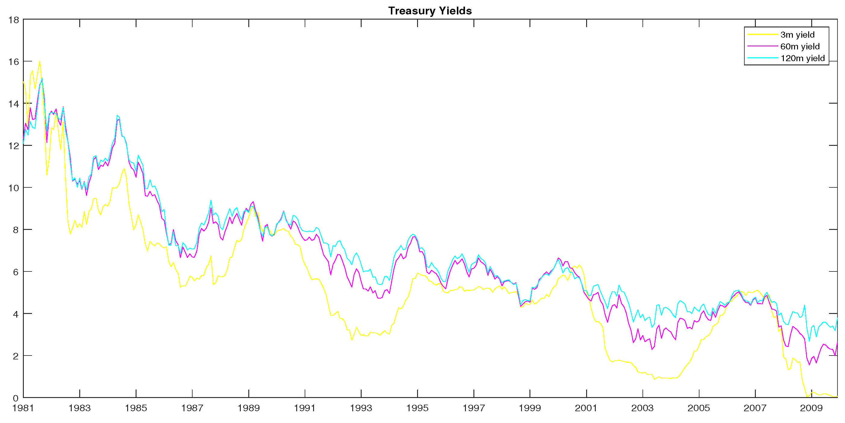
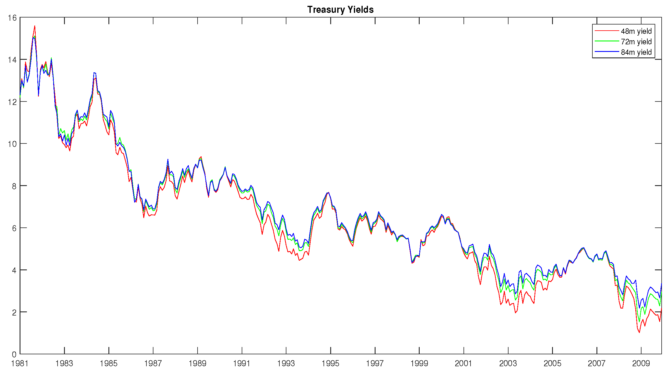
Our data set consists of fixed-maturity, end-of-month continuously compounded yields on U.S. zero-coupon bonds from January 1981 to December 2009, totaling 348 monthly observations. This data set of monthly time series of yields was constructed from [39] from the Center for Research in Security Prices (CRSP) unsmoothed Fama and Bliss [40] forward rates and is publicly available in the Journal of Applied Econometrics Data Archive (these data, denoted here as JKV data set, can be downloaded from the following link: http://qed.econ.queensu.ca/jae/datasets/jungbacker001/ (accessed on 10 October 2022)). For our work, we have chosen yields with maturities 3,48,60,72,84 and 120 months for the time period from January 1981 to December 2009. The class of Gaussian ATSMs we use in our analysis provides a good fit jointly to macroeconomic factors and bond yields. However, it has the shortcoming when some interest rates are near their zero lower bound (ZLB), placing positive probabilities on negative interest rates [41]. This condition may be problematic for the prediction of future bond yields when interest rates are very close to the ZLB: for example, in U.S. Treasury yields after the financial crisis of 2008–2009. Ref. [41] found that the standard Gaussian ATSM model performed well until the end of 2008 but underperformed since then until 2014. As a result, we choose the period until the end of 2009 in order to perform our analysis. Figure 1 and Figure 2 plot the time series of U.S. Treasury yields. The average yield curve is downward sloping. Usually, in periods where the yield curve level displays a downward trend, bond returns exhibit good performance [8].
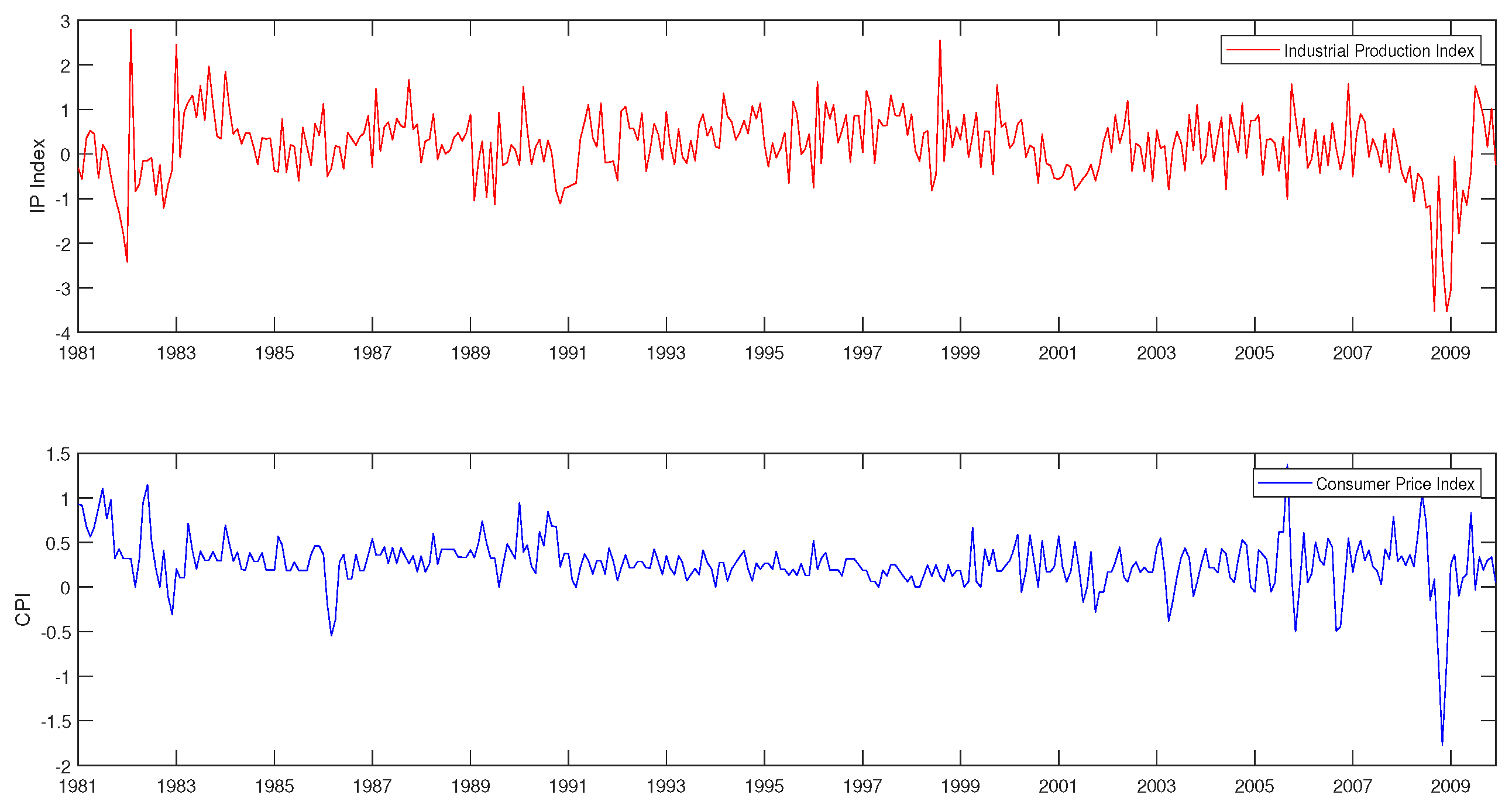
Following the recent literature, in the term structure models, we use both macroeconomic and latent factors. Since the seminal work of [42], there has been growing literature for incorporating macroeconomic factors in the term structure models (e.g., [43,44,45]). These studies exploit small macroeconomic information sets, and some authors consider the dynamics of the term structure augmented with additional factors such as information on exchange rates or survey data (e.g., [46,47,48]). Refs. [49,50] modeled yield curve dynamics by adding to standard macroeconomic factors three additional financial factors: credit risk, liquidity risk and risk premium factors ([51]). The incorporation of macroeconomic factors contributes to the improvement of yield curve forecasting. Good yield curve predictions are important in order to achieve better results in terms of fixed-income portfolio performance. We use two macroeconomic factors: Consumer Price Index (CPI) monthly time series seasonally adjusted and, as a proxy for the monthly gross domestic product growth (GDP), the monthly Industrial Production (IP) growth. The CPI measures the average changes in the price level of a basket of goods. The IP growth measures the growth rate of the production of goods. The IP growth rates and the CPI time series are obtained from the Federal Reserve St. Luis database. The data series are displayed in Figure 3. The CPI factor peaks in early 1981 and in average falls during the recession of 1981–1982. In the subsequent period, an upward trend follows before the fall in the fourth quarter of 1990. Next, the CPI stays mainly at the same level until an upward trend during the period from the end of 1999 until March 2008. For the period from the third quarter of 2008 until middle of 2009, we have a period of economic downturn due to the global financial crisis of 2008–2009. The IP index growth rate is seasonally adjusted. Most of the movements of the IP index growth rate follow that of the business cycles. However, the time series of CPI has more smooth fluctuations.
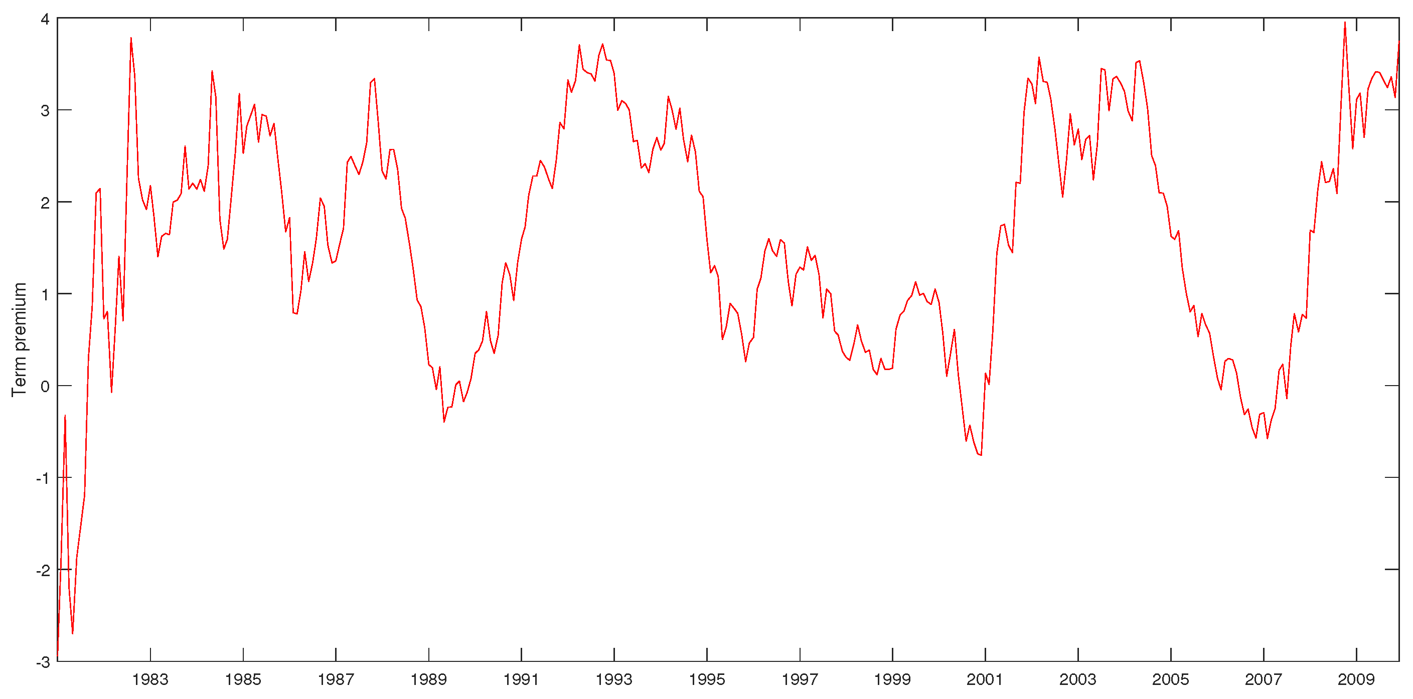
Table A1 and Table A2 present some descriptive statistics for the bond yields and the macroeconomic observable factors, respectively. The yield levels show mild excess kurtosis at short maturities, which decreases with maturity, and positive skewness at all maturities. In Table A3 and Table A4, we present the autocorrelations of these time series for lags 1, 5, 12, 20 and 24. An important fact is that the time series of all bond yields are highly autocorrelated, showing strong persistence. For lags 1 and 5, IP growth rates exhibit a low level of autocorrelation, and for lag 1, the CPI exhibits a medium level of autocorrelation. For lags greater than 5, both factors exhibit no autocorrealtion. In Figure 4, we have plotted the yields term premia, the difference between the 10-year yield and the 3-month yield. The term premia at the beginning of our sample period starts from a negative position and continuously increases from 1981:09 to 2009:12 and remains at positive levels with the exception of time periods 1989:05 to 1989:07, 1989:10 to 1989:11, 2000:07 to 2000:12 and 2006:07 to 2007:04. During the recession periods, the term premia exhibits an upward trend. The estimation procedure is performed for the in-sample period from 1981:01 to 1999:12, while the out-of-sample period is from 2000:01 to 2009:12.

4. No-Arbitrage Affine Term Structure Model

4.1. General Framework

We assume that the k × 1 vector of state variables X t follows a vector autoregressive evolution process:
X t + 1 = μ + ρ X t + Σ u t + 1
where u t + 1 is a Gaussian standard error term and μ is k × 1 vector, ρ and Σ are k × k matrices. The state variables are the two macroeconomic factors we previously mentioned in Section 3, CPI and IP growth, and three latent factors. Three unobserved (latent) factors explain much of the yield curve dynamics ([52]). In general, for our term structure model, we adopt the modeling approach of [53]. Following this approach, according to the authors, the Gaussian assumption for the model is a sufficient first approximation to the joint dynamics of bond yields and macroeconomic variables.
Equation (2) can be considered as a discretization of the Ornstein–Uhlenbeck stochastic differential equation
d X t = ( M A X t ) d t + Σ 0 d W t ,
where X t R k × 1 , M R k × 1 , A R k × k and W t R k × 1 is a Wiener process, while Σ 0 R k × k is a covariance matrix. In fact, using the Euler discretization scheme, for a time step h, we may obtain an approximation of (3) in terms of
X t + h X t = ( M A X t ) h + Σ 0 ( W ( t + h ) W ( t ) ) ,
Since u t : = W ( t + h ) W ( t ) is a Gaussian process, we can express (4) in as
X t + h = M h + ( I h A ) X t + Σ u t ,
which is in the form of (2) for the choice μ = M h , b = ( I h A ) , Σ = Σ 0 , and renaming t + h to t + 1 .
Similar considerations apply for other popular numerical schemes, such as for instance the implicit Euler scheme, according to which
X t + h X t = ( M A X t + h ) h + Σ 0 ( W ( t + h ) W ( t ) ) ,
which can be rearranged as
X t + h = ( I + h A ) 1 M h + ( I + h A ) 1 h X t + ( I + h A ) 1 Σ 0 ( W ( t + h ) W ( t ) )
which is the form (2) for μ = ( I + h A ) 1 M h , ρ = ( I + h A ) 1 h , Σ = ( I + h A ) 1 Σ 0 .
Standard results from the numerical analysis of stochastic differential equations (see e.g., [54]) imply that such discretizations converge as h 0 to solutions of the continuous Ornstein–Uhlenbeck equation (in various senses). Hence, we can stipulate that the results obtained for problem (2) in the appropriate limits can be generalized for the continuous versions of the process. This is, however, a subject for future research.
We consider the following two representations of Equation (2) under the risk-neutral pricing measure Q and under the physical probability measure P :
X t + 1 = μ Q + ρ Q X t + Σ u t + 1 Q
X t + 1 = μ P + ρ P X t + Σ u t + 1 P
The vector of state variables X t that describes the economy is partitioned into observables X t o and unobservables or latent variables X t u . The time-varying market prices of risk, λ t , are affine functions of the underlying state variables X t :
λ t = λ 0 + λ 1 X t
where λ 0 is a k × 1 vector and λ 1 is an k × k matrix. The relation of the parameters of the P -measure to the Q -measure are given by:
μ Q = μ P Σ λ 0
ρ Q = ρ P Σ λ 1
In addition, we assume that the short rate is an affine function of the state variables:
r t = δ 0 + δ 1 X t
where δ 0 is a scalar and δ 1 is an k × 1 vector. The pricing kernel in the affine term structure model is
M t , t + 1 = e x p ( r t 1 2 λ t λ t λ t u t + 1 )
with λ t = 0 in the case of risk neutrality. The pricing kernel allows us to price any asset in the economy such as nominal bond prices. Bond prices are also affine functions of the state variables and can be estimated as follows
P t n = E t ( M t + 1 P t + 1 n 1 ) = e x p ( a n + b n X t )
where
a n + 1 = a n + b n ( μ Σ λ 0 ) + 1 2 b n Σ Σ b n δ 0
b n + 1 = b n ( ρ Σ λ 1 ) δ 1
with a 1 = δ 0 and b 1 = δ 1 . Now, the yield of an n-period zero coupon bond is:
Y t n = log P t n n = A n + B n X t
where A n = a n n and B n = b n n .
Following [10], the measurement specification for Equation (18) is defined as
Y t 1 Y t 2 = A 1 A 2 + B 1 B 2 X t o X t u + 0 Σ e u t e
where Σ e is typically taken to be diagonal. A i and B i , i = 1 , 2 , are calculated by stacking (16) and (17), respectively, for the appropriate n. Σ e determines the variance of the measurement error with u t e N ( 0 , I N e ) . In order to estimate our model, we follow the approach of [55] according to which Equation (18) holds exactly for as many yields as the number l of latent factors. The remaining observed yields differ from the predicted value by a small measurement error. The choice of the maturity sets measured with error or not is driven by the interest in obtaining good forecasting of the 10-year yield. As a result, in our model, we assume that yields maturing at 3, 60, 120 months are priced without error and yields with maturities of 48, 72 and 84 months are priced with error. Let Y t 1 denote the l × 1 vector consisting of those linear combinations of yields that are priced without error and Y 2 denote the remaining ( N e × 1 ) linear combinations that are priced with measurement error. We also maintain the parameter restrictions imposed by [10,56]. These are Σ l m = 0 , Σ l l = I N l , δ 1 l 0 , μ l Q = 0 where Σ mm is lower triangular matrix. The notations l and m denote the partitions for the latent and macro factors, respectively.
Table A5 presents the mapping between structural and reduced form parameters. When the number of parameters in the structural form of the model is equal to the number of reduced-form parameters, then the model is just identified. The reduced form parameters are collected in a vector π and can be estimated by least squares methods. Then, the vector of the structural parameters θ = { μ , ρ , Σ , μ Q , ρ Q , δ 0 , δ 1 } can be estimated by the minimum chi square method. The main assumption of the method is that the reduced form parameters are equal to a function of the structural parameters, π ^ = g ( θ ) . The minimum chi square method uses the Wald test in order to test the hypothesis that π = g ( θ ) . The MCSE is then given by:
min θ T ( π ^ g ( θ ) ) R ( π ^ g ( θ ) )
where R is the information matrix of the full information maximum likelihood function L ( θ ; Y ) . The minimal value that is found by this estimator would have an asymptotic χ 2 ( q ) distribution under the null hypothesis where q is the dimension of π (for more details, see [10]).
Since we estimate the model parameters, we can estimate the coefficients α n , b n from the recursive Equations (16) and (17). The results of the parameter estimation under the risk-neutral and historical probability measure are presented in Table A6.

Forecasts

After the estimation, we try to test the forecasting ability of our yield curve model. The estimation of forecasts for our model is a crucial procedure for the estimation of the moments of bond returns and consequently for the portfolio optimization. We implement an out-of sample forecast for a period of 120 monthly time series of yields, from 2000:01 to 2009:12. In order to examine the forecasting ability of our model, we calculate the root mean square errors (RMSE) and the mean absolute error (MAE). Table 1 presents the results for RMSEs and MAEs for the yields with maturities of 3 months and 4, 5, 6, 7 and 10 years. Lower values of RMSE and MAE denote better forecasts. Root mean square errors are estimated according to the following equation
R M S E = 1 T t = 1 T ( Y ^ t n Y t n ) 2
where Y ^ t n and Y t n are the predicted and the actual yields, respectively, of a bond with maturity n months, and T indicates the total length of the forecasting period, which here is 120 months. The mean absolute errors are estimated as
M A E = i = 1 T | Y i Y ^ i | T
From Table 1, we can generally conclude that our term structure model with the two macroeconomic factors and three latent factors gives satisfactory forecasting results for the six maturities that we have. The results presented are for annualized data.
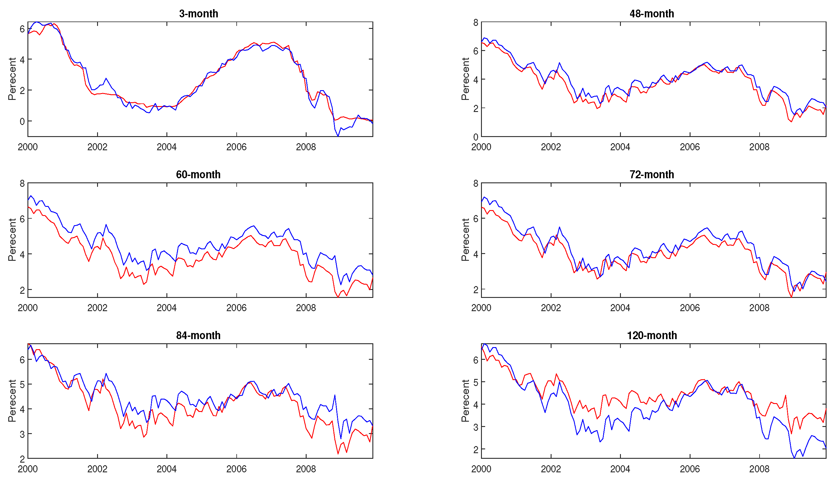
Figure 5 presents the actual bond yields versus the estimated bond yields for the out-of-sample period 2000:01 to 2009:12. For the 3-, 48-, and 72-month yield, the fitting is almost identical. The fitted 60-month bond yield is very close to the actual and mimics its course. The 84-month bond yield is almost identical to the actual except for the period 2002:03 to 2005:10 when there is a small deviation. Finally, for the 120-month yield, the deviation between the fitted and the actual yields is larger than the 84-month yield but generally performs well.

4.2. The Distribution and Estimation of Bond Returns

The main problem of fixed-income portfolios is the prediction of the distribution of asset returns for a set of maturities and the selection of the optimal portfolio weights conditional on expected returns and risk preferences. As a consequence, this requires the estimation of the expected asset returns for each maturity and their covariance matrix. The ATSM that we previously presented can be used for the construction of a fixed-income portfolio. In this section, we derive closed-form expressions for the one-period ahead expected log-returns of bonds and their covariance matrix based on the affine dynamic factor model. These estimates are key concepts to the problem of bond portfolio optimization. Following the discussion in [8], we can obtain expressions for expected bond returns and their covariance matrix based on the distribution of the yield curve model. Specifically, we are interested in the distribution of one-step-ahead forecasts of continuously compounded zero-coupon bond yields.
The Gaussian ATSM for bond yields presented in the following equation
Y t 1 Y t 2 = A 1 A 2 + B 1 B 2 X t o X t u + 0 Σ e u t e
implies that the distribution of one-step-ahead forecasts of continuously compounded zero-coupon bond yields is the normal distribution (for the estimation of the moments of bond yields, see Appendix A).
So, the one-step ahead forecasts of bond yields Y t + 1 | t N ( μ Y t + 1 | t , Σ Y t + 1 | t ) with mean and variance given by
μ Y t + 1 | t = A n + B n X ^ t + 1 | t
and
Σ Y t + 1 | t = B n S t + 1 | t B n + Σ
respectively, where X ^ t + 1 | t = E t [ X t + 1 ] denotes the expected value of the state factors X t based on the estimates from the term structure model of Equation (2). S t + 1 | t is the covariance matrix not of the true factors X t but of the filtered states based on the predicted state factors X ^ t + 1 | t ([8]). The covariance of the predicted states is given by S t + 1 | t = Σ Σ + ρ Q Σ ρ n Q . We remind that in our affine model, as we see from Equation (2), we assume homoscedasticity. As we mentioned earlier, in order to apply the mean-variance (MV) optimization approach, we need the estimation of expected bond returns and their covariance matrix. For this procedure, we need to estimate the one-period ahead of log-bond returns. We assume that the investor’s one-period return comes from holding a bond from period t to t + 1 while its maturity decreases. The log-return r i , t of holding a bond from period t to t + 1 while its maturity decreases from i to i 1 , i = 2 , , N , is
r i , t = log P t + 1 i 1 P t i = log ( P t + 1 i 1 ) log ( P t i ) = ( i 1 ) Y t + 1 i 1 + i Y t i
One-step-ahead forecasts of log-returns of bonds are normally distributed with mean given by
r i , t + 1 | t = ( i 1 ) · μ Y i 1 , t + 1 | t + i · Y t 1 i
The positive definite covariance matrix Σ r t + 1 | t has diagonal elements given by:
σ r i , t + 1 | t = ( i 1 ) 2 ( b i 1 S t + 1 | t b i 1 + σ i 1 2 )
and non-diagonal elements
σ r i , r j = ( i 1 ) ( j 1 ) ( b i 1 S t + 1 | t b j 1 + σ i 1 , j 1 )
where σ i 1 2 is the ( i 1 ) th diagonal element of Σ and ( b n i 1 S t + 1 | t b n j 1 σ n i 1 n j 1 ) is the ( i 1 , j 1 ) element of the covariance matrix Σ μ t + 1 | t of expected bond yields. The choice of the set of maturities depends among others on the investment horizon of the investor.

5. Fixed-Income Portfolio Optimization

In this section, we adopt the MV and GMV portfolio optimization approach allowing or not short selling for the construction of optimal bond portfolios based on the Gaussian ATSMs proposed by [10]. The results for the expected bond yield returns and the covariance obtained in the previous section are used for the bond portfolio optimization. The proposed MV and GMV bond portfolios are compared with traditional yield curve strategies, and its performance is evaluated.

5.1. Portfolio Framework

The portfolio theory introduced by [57] provides a basis for portfolio selection and optimization in a single-period set up. The Markowitz’s approach assumes an investor that needs two main key ingredients in order to construct an investment portfolio: (i) the estimated expected return for each investment and (ii) the covariance matrix of returns. The fixed maturity of bonds means that all bonds having maturities less than the investment horizon T 1 will not exist at time T 1 . Bond prices are functions of time and interest rates, and so, they become non-random at the maturity date. Ref. [9] considers that the major problem of a fixed-income portfolio optimization is that of constructing the variance–covariance matrix of bond returns. As a consequence, traditional portfolio optimization models such as the Markowitz portfolio method cannot be used directly for the construction of fixed-income portfolios and modifications should be used. In our work, we assume, at the time of the portfolio selection, that investors are only concerned with the expected returns of U.S. Treasury yields for the one-step-ahead forecast horizon and its variance–covariance matrix. The rebalancing frequency is 3 months.
The GMV portfolio is the portfolio with the smallest variance for a given covariance matrix of asset returns ([58]). The optimal portfolio weights are determined independently from the expected asset returns. This has the advantage that the optimization depends completely on the covariance matrix of asset returns. The covariance matrix can be estimated with more reliability than expected returns ([33]). The GMV portfolio is given from the following minimization
minimize w t w t Σ r t + 1 | t w t subject to w t 1 = 1 w t 0
where the last inequality is valid when short selling is not allowed. The optimal weights for the GMV portfolio when short selling is allowed are given by
w = Σ r t + 1 | t 1 1 1 Σ r t + 1 | t 1 1
The result of this optimization gives the vector of the optimal weights for each time period. The GMV portfolio is the only portfolio of the efficient frontier that does not depend on the expected returns and has the lowest volatility. In our work, we estimate the GMV portfolio for both the cases of allowing or not short selling on assets. Allowing short selling, we have a better portfolio performance in terms of expected return and volatility compared to the constrained GMV portfolio. However, this results in higher transaction costs and portfolio turnover rate.
In general, the mean variance portfolio problem can be formulated by minimizing the portfolio variance for a particular one-step-ahead expected bond return, subject or not to a set of additional restrictions on the vector of optimal weights w t . The mean variance framework in case that short selling is not allowed (constrained portfolio) has the following form
minimize w t w t Σ r t + 1 | t w t δ w t μ r t + 1 | t subject to w t 1 = 1 w t 0
where μ r t t + 1 | t is a N × 1 vector of expected returns of maturities n i , i = 1 , , N , and N is the number of yield maturities. Σ r t t + 1 | t is a N × N variance–covariance matrix of expected returns estimated from Equations (28) and (29) and 1 is a N × 1 vector of ones, and δ is the risk aversion coefficient. In the case where short selling is allowed in the last restriction in (32), w t can take negative values. The optimization problem in both cases is subject to a budget constraint, which ensures that all wealth is invested in the investment assets. The mean variance portfolio problem as we see from (32) solves a quadratic utility function. The mean variance problem can be stated as a myopic single-period problem where portfolio weights are calculated based on one-step-ahead bond return forecasts. In addition, when an investor changes the composition of its portfolio over time, it is then faced with transaction costs, and these costs are a function of the frequency and magnitude of asset allocation changes in the portfolio. The portfolio turnover is estimated as
T r = 1 T 1 t = 1 T 1 i = 1 N ( | w i , t 1 w i , t | )
The transaction costs are set to 3 basis points (bps) per transaction. Then, the cost of a trade over all assets is
T c = 0.003 t = 1 T 1 i = 1 N ( | w i , t 1 w i , t | )
Later, in our portfolio monitoring analysis, we focus on the GMV portfolio. This is due to the fact that expected portfolio returns are more difficult to estimate than the variance of returns and the latter can be estimated more precisely [58]. The MV portfolio framework contains the risk aversion coefficient which reflects the investor’s perception of risk. The GMV portfolio corresponds to a fully risk-averse investor who aims to minimize the variance without taking into consideration the expected return.

5.2. Benchmark Portfolio Strategies and Portfolio Evaluation Performance

The relative performance of the proposed bond portfolio strategy based on the Markowitz’s portfolio theory is compared with a set of yield curve strategies (for more information about traditional yield curve strategies, see [9,59]). We consider the following yield curve strategies: barbell strategy, bullet strategy and ladder or equally weighted portfolio strategy. The main purpose of these strategies is to reduce yield volatility and risk. In the barbell portfolio strategy, the maturity of the bonds included in the portfolio is equally weighted in the two extreme maturities, the 3-month and the 10-year bond. In the bullet strategy, the maturity of the bonds in the portfolio is concentrated at one point on the bond yield curve. This strategy means that the investor can invest either in 48-month or 60-month or 72-month or 84-month bonds, totaling four alternative portfolios. Finally, in the equally weighted portfolio strategy, the portfolio is constructed so as to have an equal amount of each yield maturity.
The empirical implementation of the mean variance optimization problem defined by (32) is performed by using one- step-ahead estimates of the vector of expected returns and its covariance matrix, considering alternative values for the risk aversion coefficient δ , 0.0001, 0.01, 0.1, 0.5, 1, 2 and 4.
The performance of optimal mean variance and minimum variance portfolios is evaluated using the average portfolio return ( μ r ), the average excess return with respect to the risk-free rate ( μ e x ) and the Sharpe ratio (SR). We consider the risk-free rate to be the Federal Funds rate. These statistics are calculated as
μ r ^ = 1 T 1 t = 1 T 1 w i , t R t + 1 μ ^ e x = 1 T 1 t = τ T 1 ( w t R t + 1 r t + 1 f ) S R = μ ^ e x σ ^
where r f is the risk-free rate, which in our case is the federal feds rate, and w t is the vector of weights in the portfolio in period t. R t = [ r 1 , t , , r N , t ] is a vector with the bond returns of all maturities and σ is the standard deviation of the portfolio’s excess return.

5.3. Results for MV and GMV Portfolios

We now present the optimal mean variance portfolios for the out-of-sample period, totaling 120 months, for the JKV data set and for different levels of the risk-aversion coefficient δ . Optimal portfolio compositions are rebalanced on a 3-month basis. First, we estimate the optimal weights under the mean-variance framework for both allowing or not short selling and subsequently the optimal weights for the GMV portfolio. The excess return is calculated using the Federal Funds rate, as the risk-free asset and the level of transaction costs is set to 3 bps. The results presented here for the mean variance portfolio are for risk aversion δ = 0.001 .
Table 2 reports the following monthly performance measures: mean gross return, mean net excess return, portfolio standard deviation and the Sharpe ratio of the proposed portfolio strategy for both the cases allowing short selling or not. The table includes the results for the barbell strategy, the portfolio strategy of investing in the maturities remaining after excluding the 3-month and the 10-year bond (portfolio strategy A). In addition, Table 2 reports the performance measures for the ladder portfolio strategy and a bullet strategy investing either in a 4-year, 5-year, 6-year or 7-year bond. The results show that our portfolio strategy (ATSM-MV) based on the ATSM produces returns and Sharpe ratios higher from many of the other benchmark strategies. Table 2 shows that the optimal mean variance portfolio of U.S. Treasury bonds achieved a mean monthly average gross return of 9.83% for unconstrained portfolio and 9.89% when short selling is not allowed. The monthly standard deviation is 1.815% and 1.785%, respectively. The risk-adjusted performance is measured by the Sharpe ratio, which is equal to 4.71% and 5.44% for unconstrained and constrained portfolios, respectively. The results indicate that our proposed mean-variance bond portfolio strategy can be a very good alternative to many traditional portfolio strategies.
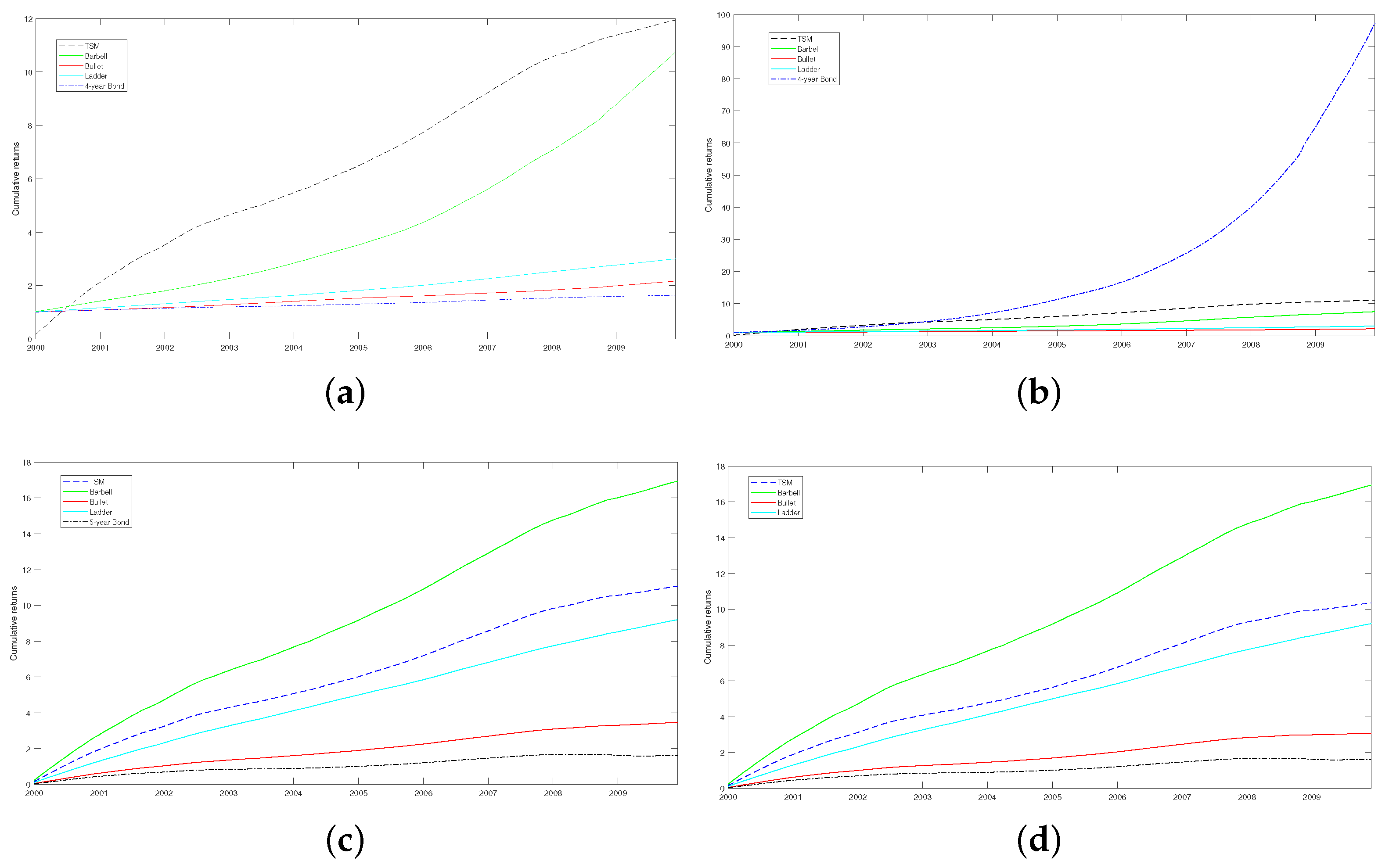
Figure A3a illustrates for the case of no short selling the cumulative returns of optimal portfolios estimated through our term structure model in comparison with some basic benchmark portfolio strategies. Specifically, we have estimated the cumulative returns following the barbell, A and ladder portfolio strategy. The cumulative returns of the mean variance portfolios obtained from the term structure model using the minimum chi-square method outperform the other strategies for the out-of-sample period. In case of short selling (see Figure A3b), again, our method outperforms the others. For both cases, cumulative returns exhibit similar patterns.
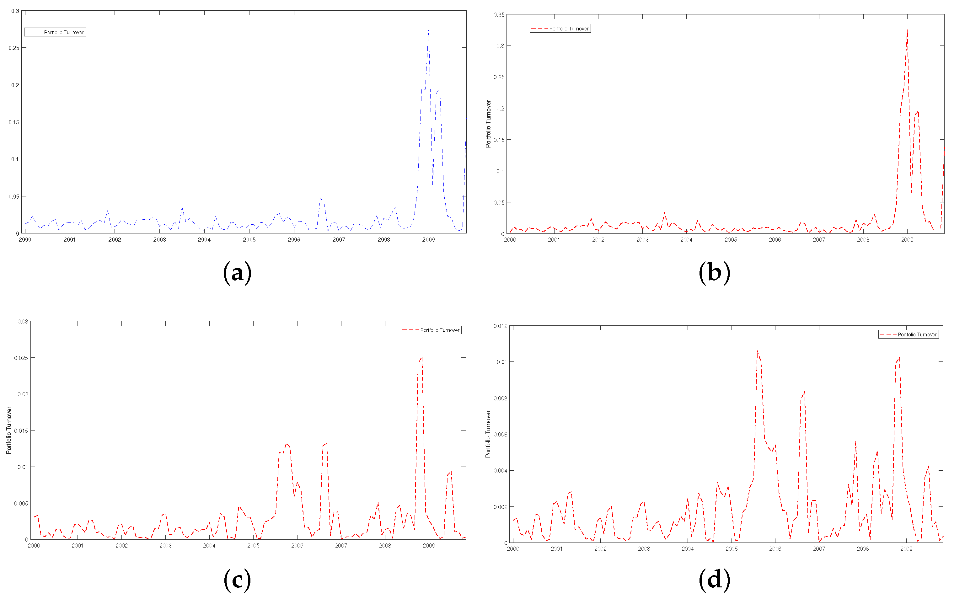
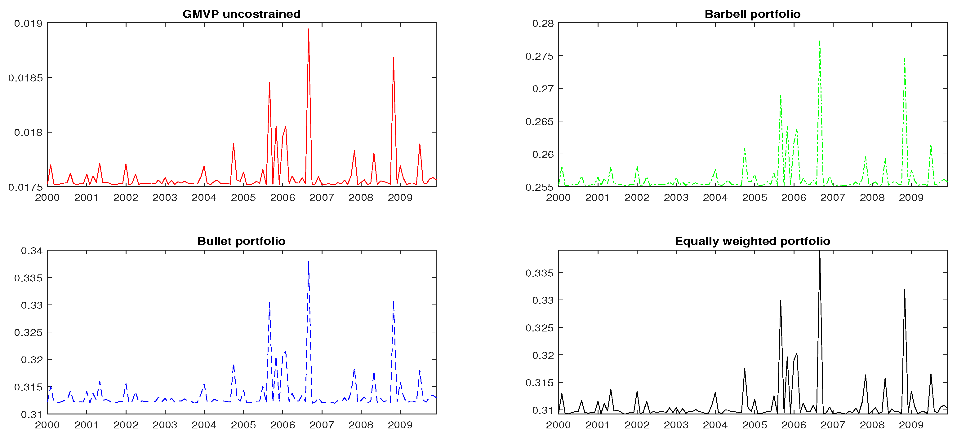
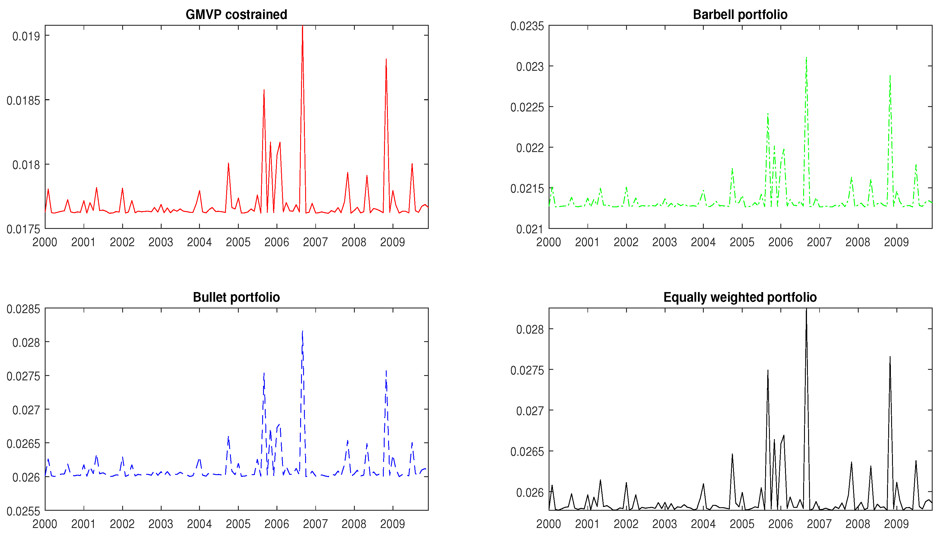
In addition, Table 2 presents the performance measures for the unconstrained and constrained GMV portfolio. The results show that our portfolio strategy based on the affine term structure model (ATSM-GMV) performs quite well in terms of mean returns, since only the barbell portfolio strategy outperforms our strategy but at the cost of higher portfolio standard deviation. The performance of the GMV portfolio constructed via an ATSM is compared in terms of cumulative returns, for the entire out-of-sample period, with other benchmark portfolio strategies (see Figure A3c,d). The results favor our method of GMV optimal portfolios either with short selling or not. In the GMV portfolio strategy, the term structure-based method performs in terms of monthly returns quite satisfactory, and only the barbell strategy outperforms ours. The results show that in terms of mean gross and excess returns, only the barbell strategy performs better than our strategy. The Sharpe ratio with our approach is larger than that of the barbell strategy. A comparative analysis of the performance of MV and GMV portfolios shows that the first generates higher Sharpe ratios, but the latter exhibits a lower standard deviation. The evolution of portfolio allocation shows that as in the MV portfolio optimization, the position of the investor is concentrated in holding a 48-month bond at time t and a 3-month bond at time t + 1 but now in lower levels. In addition, our portfolio strategy for the entire out-of-sample period produces lower standard deviation from the barbell, bullet and ladder portfolio strategies (see Figure A1 and Figure A2). The portfolio turnover in both the unconstrained and constrained case shows a large increase at the end of 2008 during the global financial crisis (Figure A4a,b). A much lower increase for the unconstrained portfolio arises in the middle of 2006.
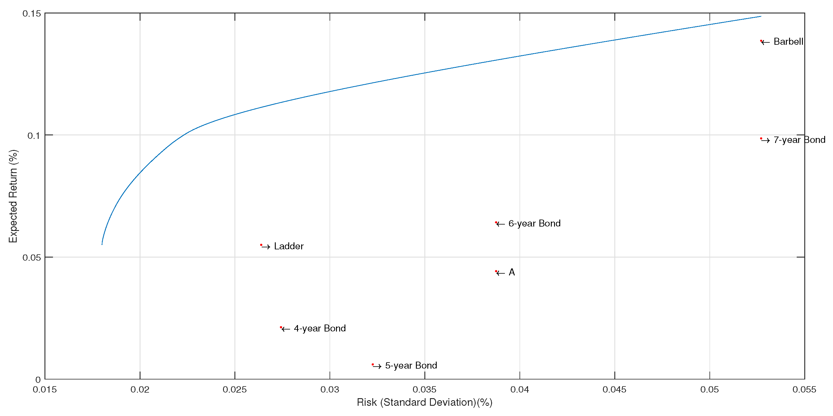
In Figure 6, we present for example the efficient frontier for a specific time period, July 2009, for the case of a constrained MV portfolio along with the benchmark portfolio strategies. We remind that the efficient frontier represents the optimal portfolios for given amounts of risk and return. Specifically, when a portfolio is on the efficient frontier, then there is no other portfolio with higher expected return and lower risk. From the graph, we see that all the benchmark portfolios lie below the efficient frontier having higher risk levels for the defined rate of return.
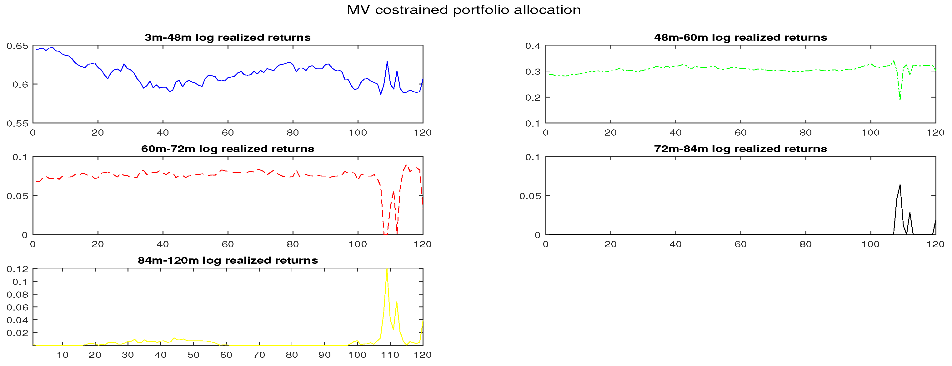
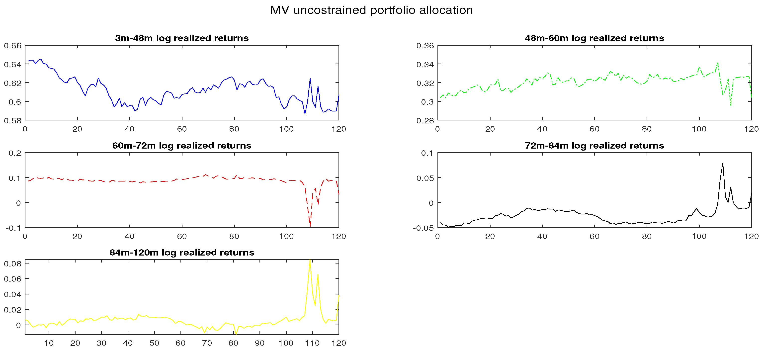
Figure A5 presents the evolution of optimal mean variance portfolio weights for the out-of-sample period under the assumption that short selling is not allowed and Figure A6 presents the evolution of optimal weights for each bond when short selling is allowed. In both cases, the investor’s position is concentrated in levels higher than 55%, holding a 48-month bond at time t and a 3-month bond at time t + 1 . In the constrained case, the weights are concentrated in investing in the first three maturities at time t and moving to a bond of the next maturity at time t + 1 . In the unconstrained portfolio case, this happens for the first two maturities.
In conclusion, the results obtained from the construction of optimal portfolios from the affine term structure presented in Section 4 can be summarized as follows. The proposed bond portfolio strategies for the MV potfolio (ATSM-MV) and the GMV portfolio (ATSM-GMV) in most of the cases produce better mean returns and Sharpe ratios with lower risk in comparison with traditional bond portfolio strategies. The results are valid regardless or not of the choice of allowing short selling.
Ref. [7] compared the results from MV and minimum MV portfolios for various rebalancing frequencies assuming different specifications for the transition equation of the factors with some benchmark indices. The average and cumulative returns of the MV portfolio exceeded those obtained by the benchmark indices with lower standard deviation. Ref. [8] applied their analysis on two bond yield data sets: one where the out-of-sample yields display a downward trend (the JKV data set) and another with an upward trend. For the JKV data set, most of the MV portfolios had risk-adjusted performance better than that of the benchmark strategies. The dynamic factor-based portfolios did not produce higher Sharpe ratios for every benchmark strategy. In our case, only the investment in a 7-year bond produced a higher Sharpe ratio than any other investment strategy but with poor performance in the risk–return tradeoff.

6. Control Charts and Optimal Weights Monitoring

In this section, we construct control chart procedures for monitoring optimal portfolio weights obtained from the method described in the previous section. Our sequential monitoring analysis is restricted to GMV optimal portfolio weights. In contrast with the MV portfolio, the GMVP weights depend only on the covariance matrix of yield returns but not on the mean yield returns, which increases the estimation risk of the portfolio. Since the investment decisions are mainly made in terms of portfolio weights, we choose to monitor the vector of optimal weights for each time period. In addition, monitoring optimal weights in government bond portfolios can be very helpful in cases of liquidity problems.

6.1. Sequential Monitoring of Optimal Portfolio Weights

Structural changes in the distribution of assets returns may have as a result changes in the optimal asset portfolio allocation. The fast detection of these changes in optimal portfolio weights has an economic effect for the investor who is interested in knowing at every time if the portfolio allocation is optimal. A very common assumption in the finance literature is that asset returns are i.i.d and follow the normal distribution. In our case, bond expected returns due to their construction from the same dynamic term structure model exhibit correlation. The results show that expected returns in most of the cases show correlation greater than 0.68 (see Table A7). In our work, we use the control charts for the first differences of [23] but with a different approach to the estimation of the covariance matrix of the control statistic. We assume that the covariance matrix of asset returns remains unchanged between two consecutive change points. The Mahalanobis distance of the first differences of the optimal weights w ^ t , n * that contains the first k 1 components of w ^ t , n , D t , n = w ^ t , n w ^ t 1 , n from the mean when the process is in-control, which is defined as
T t , n d = ( D t , n E 0 ( D t , n ) ) Ω d * 1 ( D t , n E 0 ( D t , n ) )
with Ω d * = C o v 0 ( D t , n ) , the covariance matrix when the process is in-control and Ω * denotes the ( k 1 ) × ( k 1 ) matrix obtained by dropping the k-th row and the k-th column of the matrix Ω . In addition, when the process is in-control, we have E o ( D t , n ) = 0 ; then, the Malanobis distance takes the following form
T t , n d = D t , n Ω d * 1 D t , n
The univariate EWMA recursion is given by
Z t , n d = ( 1 λ ) Z t 1 , n d + λ T t , n d
where t 1 and λ ( 0 , 1 ] .
The starting value for the control statistic is
Z 0 , n d = E 0 ( D t , n C o v 0 ( D t , n ) 1 D t , n ) = E 0 ( T t , n d ) = k 1 ,
where E 0 ( . ) is the expected value when the process is in-control.The monitoring process is out-of-control if Z t , n d > c d , c d is an appropriately chosen control limit. For the difference control charts based on the multivariate EWMA recursion, the control statistic is
Z t , n d = ( I R ) Z t 1 , n d + R D t , n , t 1
with starting value Z 0 , n d = E 0 ( D t , n ) = 0 . The process is out-of-control if
Z t , n d C o v 0 ( Z t , n d ) 1 Z t , n d > c 1 d
The control limit of a control chart defines the rejection area in every control scheme and is estimated through a simulation study for a predetermined value h of the A R L 0 . Usually, in financial applications, this A R L 0 is equal to 120 days or 1/2 year of daily observations [60]. When the control chart gives a signal, the financial analyst should investigate it and determine the next steps about the optimal portfolio composition.
We chose the in-control average run length to be equal to 6 months. This means that on average, the first false signal comes after six months of observations. The critical value c d is the solution of Equation (1). First, we choose a starting value for the control limit and we simulate the difference process of optimal weights. Next, these simulated values are applied to the control chart procedure, and the stopping times of the control charts are simulated. Finally, we simulate values of the difference process of optimal weights, and the stopping times are recorded. This simulation procedure at every step is iterated 5 × 10 4 times. The estimated ARL in the in-control state is the average of simulated stopping times. The iterations are stopped if the absolute deviation from the prespecified in-control ARL is less than an accepted level of error, which here is 0.2%. For the estimation of the control limit using the median run length (MRL), we follow the same technique as described with the ARL, and the MRL 0 is chosen equal to 6 months.

6.2. Estimation of the Covariance of Optimal Weights

The optimal portfolio weights for the MV portfolio framework depend on the unknown parameters of the asset returns distribution which are subject to unknown structural breaks. In the GMV portfolio framework, the expected portfolio return and the portfolio risk depends on the optimal weights composition on the variance of asset returns. Because the variance of asset return is unknown in practice, it has to be estimated. The parameter estimation causes an estimation risk in the optimal portfolio selection, and ignoring it may have negative consequences in optimal portfolio selection [61]. Various methods have been applied in order to reduce the estimation risk (see for example [2,62]). A very common estimator of the covariance matrix of asset returns is the sample covariance matrix. In our work, the covariance matrix of asset returns is estimated through the affine term structure model.
The main problem in order to estimate the control statistics for the difference charts we presented in the previous section is the estimation of the covariances when the process is in-control of the differences of the optimal weights. Suppose a portfolio consisting of risky assets under the assumption of independent and normally distributed returns. Since the exact estimation of the autocovariances of the control statistics we previously mentioned is difficult, [23] based on the work of [28] propose an approximation for large n. Ref. [32] mentioned that an alternative method for the covariance estimation could be a Monte Carlo approach. In our case, due to the high correlation of the asset returns we have, we choose to estimate these quantities through a simulation study. Specifically, we try to approximate the covariance matrix through a simulation study. This simulation approach requires generating data from the term structure model. The assumption of normality in the affine model makes this procedure much easier and faster. The challenging part is the definition of the in-control condition for the term structure model. Since this period is defined, we generate the state evolution process from the known mean and variance matrix of the real data. In the in-control condition, the estimation of the covariance of the control statistic Z t , n d needs the estimation of the covariance matrix between the k 1 optimal weights. Ref. [23] study and approximate the limit behavior of C o v 0 ( Z t , n d ) as n tends to infinity.
For the estimation of the autocovariance matrix of the first differences of optimal weights, we use the following iterative procedure:
(1)
Generate data from the state evolution process X t N ( μ X , Σ Σ ) when the process is in-control and μ X is the mean of the state process.
(2)
Generate residual data for the state evolution process from U N ( 0 , I ) .
(3)
Estimate the covariance matrix of the filtered states X t | t + 1 .
(4)
Estimate the covariance matrix of one-period ahead bond yields Y t | t + 1 .
(5)
Estimate one-period ahead realized returns according to Section 4.2.
(6)
Estimate optimal global minimum variance portfolio weights.
(7)
Estimate the first differences of optimal weights.
(8)
Estimate variance of first differences of optimal weights.
(9)
Repeat the above procedure.
After the estimation of the autocovariances of optimal weights from Equations (40) and (41), we can estimate the control statistics for the first difference procedures of the EWMA based on the Mahalanobis distance and the multivariate EWMA recursion.

7. Simulation Study

The proposed difference control schemes for correlated data along with their detection ability are analyzed within a simulation study. At first, the control limits for all charts are determined in such a way that the control charts provide the same in-control average run lengths, which are here assumed to be equal to a period of six months. After obtaining the control limits through simulation as described previously, the performance of control charts assuming that a change point happens at the beginning the performance is evaluated by computing the A R L 1 and the out-of-control median run length ( MRL 1 ). The optimal performance provides the smallest out-of-control average run length. A small A R L 1 value means that the control chart is capable of detecting as soon as possible the shift in the process given that the process is out-of-control.

7.1. Modeling the Out-of-Control State

In our simulation study, we follow a similar approach to that of [33] for modeling the variance of asset returns. We assume that we have m = 6 fixed-income assets, government bond yields, that follow the normal distribution with monthly in-control mean μ 0 , Y and variance Σ 0 , Y which has the following form
Σ 0 , Y = S 0 , Y · C 0 , Y · S 0 , Y
where S 0 , Y is a diagonal matrix that contains the standard deviations and C 0 , Y is the correlation matrix of bond yields. In addition, the variance of the out-of-control state has the following form
Σ 1 , Y = S 1 , Y · C 1 , Y · S 1 , Y
where S 1 = [ 0.7 h 0.8 h 0.85 h 0.9 h 0.95 h 0.99 h ] × I , and
C 1 = 1 0.403 v 0.421 v 0.433 v 0.331 v 0.0403 v 1 0.8030 v 0.8319 v 0.6757 v 0.421 v 0.8030 v 1 0.8570 v 0.7015 v 0.433 v 0.8319 v 0.8570 v 1 0.7287 v 0.331 v 0.6757 v 0.7015 v 0.7287 v 1
The numerical values in the mean, variance and correlation matrices are chosen so as to be in accordance with the real data that we have in our empirical example and described in Section 3. Here, we assume changes only in the variance of the bond yield returns, so we set v = 1 . This assumption is necessary because we did not want to reduce the correlation of assets returns, since our example refers to government bonds that due to their construction exhibit strong correlation. The standard deviation parameter h that defines the shift in the variance process can take values from the set { 1.5 , 2 , 2.5 , 3 , 3.5 , 4 , 4.5 } . For the out-of-control condition, the in-control variance Σ 0 , Y changes to the new variance Σ 1 , Y , and we estimate the out-of control optimal weights for the GMV portfolio. The estimation window n for the construction of optimal portfolio weights is equal to 40 monthly observations. The smoothing parameter in the univariate EMWA based on the Mahalanobis distance is λ { 0.05 , 0.1 , 0.15 , 0.2 , 0.25 , 0.3 , 0.35 , 0.4 , 0.45 , 0.5 , 0.75 , 0.9 } . The multivariate EWMA control charts are constructed with all smoothing parameters in the main diagonal equal, R = λ I . In our simulation study, we examine in total 84 different out-of-control cases. In each of these out-of-control cases, we apply the proposed control chart procedures and calculate the A R L 1 and the M R L 1 . We mention that these measures are calculated under the restrictive assumption that the change happens at time t = 1 .

7.2. Simulation Study Results

Ref. [28], under the assumption that the asset returns are independent and identically normally distributed, derives the exact distribution of optimal weights w ^ t and proves they are asymptotically normal. In our work, the independence of asset returns is not valid, because bond yields are estimated via a common dynamic factor model. In order to overcome this problem, we choose to follow a simulation approach for estimating the necessary moments of optimal weights.
The simulation study compares the results for the out-of-sample period of four control chart cases: the univariate EWMA control charts based on Mahalanobis distance for unconstrained (Mahalu) and constrained portfolio (Mahalc), the control charts based on the multivariate EWMA (MEWMA) statistic for unconstrained (MEWMAu) and constrained portfolio (MEWMAc). For the first case (Mahalu), the A R L 1 is reduced for each certain level of the smoothing parameter λ as the variance increases. For values λ = { 0.05 , 1 } and λ = { 0.75 , 9 } , we observe large values for the A R L 1 . In parentheses, we present the MRL 1 s , which follow the same pattern as the A R L 1 s . The results for the second case (Table A8) show that the strategy of not allowing short selling gives smaller out-of-sample A R L 1 s . Again, for a given value of the smoothing parameter, as the shock in variance increases, the A R L 1 decreases. Control charts based on the MEWMA statistic for the unconstrained portfolio exhibit lower values of A R L 1 for the Mahalanobis distance case. Finally, the fourth case (Table A9) gives the lowest A R L 1 except in the cases with smoothing parameters λ = { 0.75 , 0.9 } . Generally, the examples with portfolios not allowing short selling perform better in terms of A R L 1 than allowing short selling. The MRL 1 s for the constrained portfolios indicate that our method gives a signal at the next time period when the monitoring process of portfolio weights is already in the out-of-control state. The fact that the MRL 1 is smaller in some cases from the A R L 1 indicates that the distribution of the run length may be extremely right-skewed [23].
Table 3 presents the best A R L 1 values for each control chart case and the corresponding value of smoothing parameter λ for each shock in the variance matrix. For the Mahalu case, the control chart with smoothing parameter λ = 0.35 performs better and gives the smallest out-of-sample A R L 1 . In Mahalc, this happens for smoothing parameter λ = 0.1 . On the contrary, in MEWMAu and MEWMAc, there is no unique smoothing parameter value that outperforms the others. In the first case, small shocks are detected faster from large values of λ in contrast to larger shocks where small values of the smoothing parameter are more appropriate. In the latter, for all shocks in the variance, the best results are given for small values of the smoothing parameter. Table 3 exhibits the best MRL 1 s values for the two cases for unconstrained portfolio, Mahalu and MEWMAu, along with the corresponding smoothing parameter values. In both cases, there is no specific value for the smoothing parameter that outperforms the others.
The difference control charts based on the Mahalanobis distance perform better than those based on the multivariate EMWA recursion in the case of unconstrained portfolios. This does not always happen when short selling is not allowed, since in many cases, the control schemes based on MEWMA recursion have slightly better results in terms of out-of-sample A R L 1 . As a portfolio strategy, the prohibition of short selling has as a result a lower out-of-sample A R L 1 s and MRL 1 s . The smallest out-of-sample A R L 1 s obtained for the Mahalu control charts are comparable with the results from the MEWMAu control charts. With some exceptions, the proposed difference control schemes for monitoring optimal weights from a government bond portfolio favor small values of the smoothing parameter. This is in accordance with the results for the case of portfolios constructed from risky assets ([23]). Additionally, the difference control schemes appear to react slowly in small changes in the variance of asset returns, and the out-of-sample A R L 1 takes large values except in the case of MEWMAc.

8. Empirical Example

The control charts based on the first differences of optimal portfolio weights are applied in the out-of-sample period from January 2000 to December 2009 for a total of 120 months. We assume an investor holds a portfolio consisting of k = 6 U.S. Treasury bonds. Before we construct the control charts, it is necessary to determine the target process or else the in-control process. This may be quite challenging for real data in financial applications, especially in our example, where we have less frequent data than daily or monthly. When the monitoring process is in-control, it is assumed there is no change point and the target process is estimated.
We choose the period from September 1996 to December 1999, for a total of 40 months, as the prerun period where the process is in-control. In this period, the U.S. Treasury bond returns are assumed to be in the in-control state.This period is before the recession at March 2001 according to the National Bureau of Economic Research (NBER) (see https://www.nber.org/cycles/main.html (accessed on 10 October 2022)). Using the observations from this period, we estimate the in-control one-period ahead log-realized returns, the one-period ahead expected returns, the covariance matrix of bond returns and the target optimal GMV portfolio weights. The control charts are constructed for the out-of-sample period, and there is no-reestimation of the target process in case of a change point. After the control chart gives a signal and is confirmed from the financial analyst that this is a structural break, normally, the target process should be reevaluated (see, for example [23,33]). Since, in our case, we have less frequent data, a possible solution to this problem may be via simulation. The control limits are chosen for a prespecified value h of the A R L 0 , which is equal to 6 months: this means that on average, each control chart should give the first false alarm after six months. The control charts are estimated for the following set of smoothing parameters: λ { 0.05 , 0.1 , 0.15 , 0.2 , 0.25 , 0.3 , 0.35 , 0.4 , 0.45 , 0.5 , 0.75 , 0.9 } . Ref. [23] mentioned that a benefit of the first difference control charts is that they give an alarm almost immediately with high probability if the change in the parameters we monitor is large. The estimation algorithm is presented in Appendix B.
Ref. [63] is in favor of lower values for the smoothing parameter and found that the optimal value of λ is time varying and clusters in high and low periods. In contrast, [64] support the choice of large values of the smoothing parameters in the EWMA model in financial applications. In our empirical example, we find that in the case of control schemes based on the Mahalanobis distance, constrained and unconstrained GMVP values equal or lower than 0.15 and 0.3, respectively, are appropriate. In addition, for control schemes based on multivariate EWMA recursion for both cases, smoothing parameter values equal or lower than 0.3 are preferred.
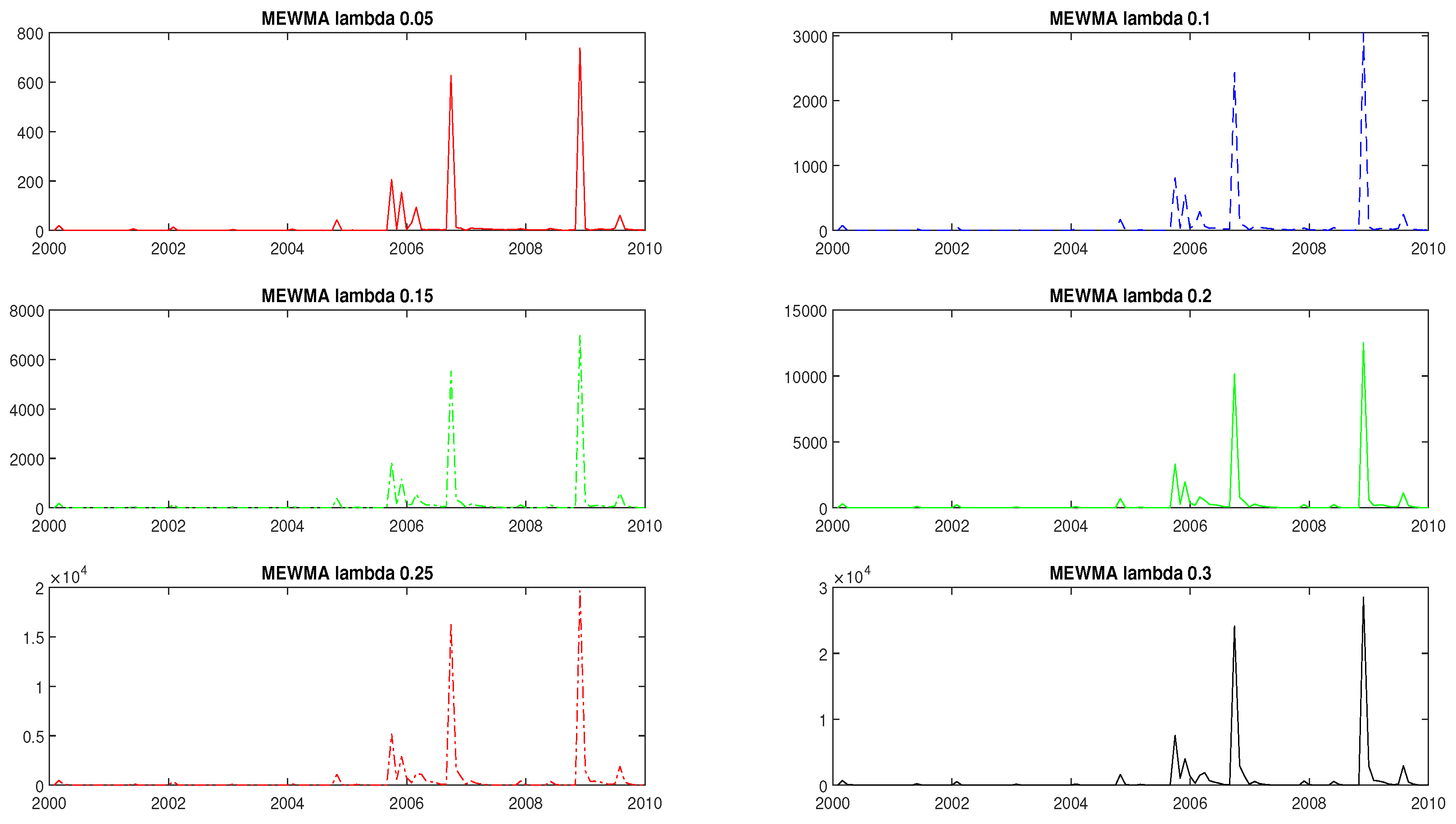
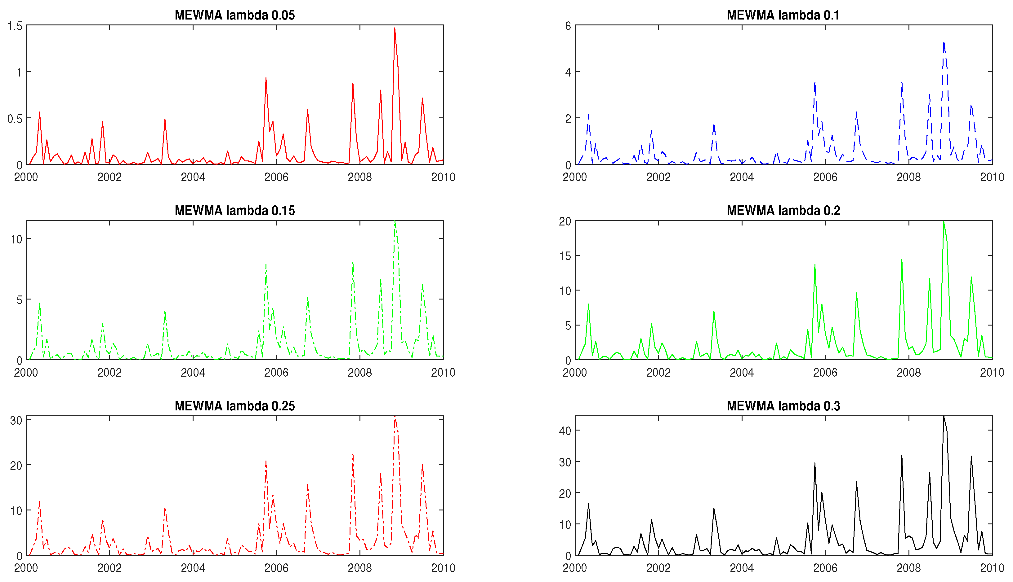
Figure 7 and Figure 8 present analogously the control statistics based on the MEWMA recursion. We remind that for the MEWMA charts, the smoothing matrix is taken as a diagonal matrix with diagonal elements equal to λ , R = λ I . In the control schemes, based on the Mahalanobis distance, the control statistics show large oscillations in contrast with those of MEWMA recursion that exhibit a very smoother behavior. As a consequence, control statistics based on Mahalanobis distance are more often lying above the control limit from those based on MEWMA recursion.
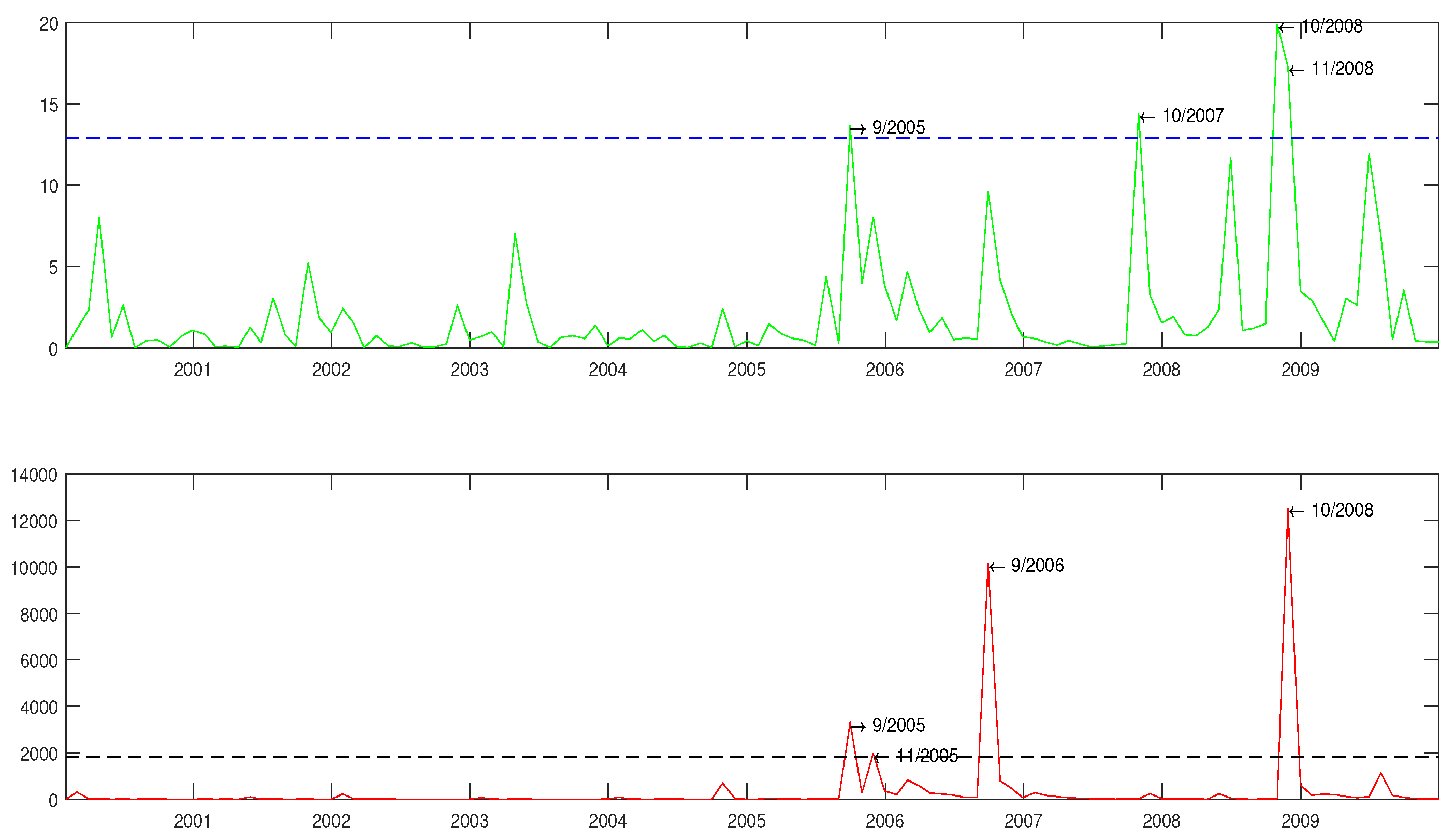
The main purpose of an investor is to minimize the one-period-ahead out-of-sample portfolio variance. The proposed control charts give a signal when a structural break in the optimal portfolio weights is likely to happen. Table 4 presents for the two control chart procedures, constrained and unconstrained portfolio optimization, the control limits and the corresponding smoothing parameters. The smoothing parameters for the procedures based on the Mahalanobis distance are set equal to 0.15, and for the MEWMA statistics, both optimization cases are equal to 0.2. Additional results for other values of the smoothing parameter are available upon request. Figure 9 illustrates the change points for the control schemes based on the MEWMA. We remind that when a signal is given and a change point is identified, the process should be re-estimated, as [23] mentioned.
Figure 9 presents the control charts for the two portfolio strategies based on the multivariate EWMA recursion. The difference control charts using the Mahalanobis distance for both constrained and unconstrained portfolios give more signals than the charts using the MEWMA statistic. The latter control schemes behave better, which is in contradiction with the results for risk assets and daily data that [23] found. A possible explanation could be the difference in the risk characteristics of the data, since here, we have less risky assets than stocks: government bonds. A possible advantage of using less frequently than daily data could be the reduction of a large number of signals especially in terms of structure models. A distinction between real and false alarm, is difficult and each signal obtained should be evaluated for further actions by a financial analyst. In our work, we attempt to give, if it is possible, an economic interpretation of the signals obtained from the control charts. The use of a difference MEWMA control chart for an unconstrained portfolio gives in the out-of-sample period four signals (without reestimation). The dates of the signals are 2005:09, 2007:10, 2008:10 and 2008:11. The difference MEWMA control chart for a constrained portfolio gives signals at the following dates: 2005:09, 2005:11, 2007:09 and 2008:10. The economic evaluation of all given signals is of great importance in finance. In December 2007, the global financial crisis started, which led to the Great Recession until June 2009 according to the NBER. Both control schemes detect the structural break due to the financial crisis of 2007. However, the MEWMA chart for the constrained portfolio gives a signal a month earlier than the chart in an unconstrained case. The signals that both charts give in September 2005 could be associated with the housing market correction during the period 2005–2006 that started in June 2005.
If we estimate the Sharpe ratios for the constrained and unconstrained GMV portfolio for the time periods before and after the change point at September 2005, we see a decline in the values (see Table 5). This is an extra indication that the financial analyst should examine the composition of the optimal portfolio. Specifically, from the results in Table 5, we see that ignoring a structural break may have important economic consequences for the investor, since the performance of the investment has deteriorated, and the optimal portfolio allocation has changed. From Figure A1 and Figure A2, for the unconstrained and constrained GMV portfolio, respectively, we see fluctuations and a rise in the portfolio standard deviation from September 2005 until the end of the out-of-sample period.
The number of signals that detect previous works about monitoring stock portfolios with control charts (e.g., [23,33]) is quite large, especially in comparison with our analysis about term structure-based portfolios. This can make the work of an analyst more difficult so as to explore the causes and the results of each detected change from the control chart.

9. Concluding Remarks

In this work, we first apply the mean variance portfolio approach introduced by Markowitz ([57]) to obtain optimal portfolios composed of government bonds. The portfolio optimization is based on an affine term structure model estimated using the minimum chi square approach. The research is restricted to the class of Gaussian VAR affine term structure models using both latent and macro factors. For the state evolution process, we assume homoscedasticity. This portfolio optimization strategy is compared with other benchmark strategies and outperforms most of them for both allowing short selling or not. In addition, the results confirm the finding of previous works (e.g., [7,8]) that portfolio optimization based on dynamic factor models could be an alternative to traditional bond strategies. Second, we propose control charts for the surveillance of optimal portfolio weights based on the differences between two successive estimated global minimum variance portfolio (GMVP) weights. We apply these control schemes in two portfolio optimization cases, allowing short selling or not. The difference control charts are based on the univariate EWMA recursion using the Mahalanobis distance and the multivariate EWMA recursion.
The estimation of the control charts requires the knowledge of the moments of the estimated optimal weights and especially their autocovariance. For the estimation of the covariance, we use a simulation approach, since our asset returns are correlated. The proposed control schemes are constructed so as to have the same in-control average run length (ARL) or media run length (MRL). Next, they are compared using as a performance measure the out-of-control ARL and MRL. For the out-of-sample period, only changes in the variance of bond returns are considered. The MEWMA difference control chart performs better than the the Mahalanobis difference chart, and for every control scheme, the results for a constrained portfolio outperform those for an unconstrained. The smoothing parameter values should be chosen from the interval 0.1 to 0.3. In addition, an empirical study is performed with the results for the out-of-sample period favoring the MEWMA difference control chart and the Malananobis difference charts giving a larger number of signals. Previous works for stock portfolios that use EWMA control charts, such as those of [23], support the use of difference control chart procedures with values for the smoothing parameter within the interval [0.1,0.25]. An important issue is the economic interpretation of the signals and the identification as structural breaks or not.
Finally, further research should be focused on techniques for the estimation of the moments of optimal portfolio weights when the asset returns are identical and data-dependent under the normality assumption. In addition, further analysis should be extended to non-Gaussian affine models or models that allows heteroscedasticity.
Author Contributions

Conceptualization, K.B., S.P. and A.N.Y.; Data curation, K.B., S.P. and A.N.Y.; Formal analysis, K.B., S.P. and A.N.Y.; Investigation, K.B.; Methodology, K.B., S.P. and A.N.Y.; Resources, K.B.; Software, K.B.; Supervision, S.P. and A.N.Y.; Writing—original draft, K.B.; Writing—review & editing, K.B., S.P. and A.N.Y. All authors have read and agreed to the published version of the manuscript.

Funding

This research received no external funding.

Institutional Review Board Statement

Not applicable.

Informed Consent Statement

Not applicable.

Data Availability Statement

The data set consists of continuously compounded yields on U.S. zero-coupon bonds that was used in this study is publicly available online at the following link: http://qed.econ.queensu.ca/jae/datasets/jungbacker001/ (accessed on 10 October 2022). The data for the macroeconomic factors are from the Federal Reserve Bank of St. Louis, publicly available on the website: https://fred.stlouisfed.org (accessed on 10 October 2022).

Conflicts of Interest

The authors declare no conflict of interest.

Appendix A. Moments of Bond Yields

Suppose that the yield of an n-period zero coupon bond is given by
Y t n = A n + B n X t + ϵ t , ϵ t N ( 0 , Σ Y ) .
The expected value is
E t 1 [ Y t ] = A n + B n E t 1 [ X t ] = A n + B n X t | t 1 ,
where X t | t 1 is the one-step-ahead predictions of the state factors.
The conditional covariance matrix of bond yields is given by
Σ Y t = E t 1 [ Y t E t 1 ( Y t ) ] [ Y t E t 1 ( Y t ) ] = E t 1 [ A n + B n X t + ϵ t A n B n E t 1 ( X t ) ] [ A n + B n X t + ϵ t A n B n E t 1 ( X t ) ] = E t 1 [ B n X t B n E t 1 ( X t ) + ϵ t ] [ B n X t B n E t 1 ( X t ) + ϵ t ] = E t 1 [ B n X t B n ( μ + ρ X t 1 ) ] [ B n X t B n ( μ + ρ X t 1 ) ] = E t 1 [ ( B n ( X t μ ρ X t 1 ) + ϵ t ) ( B n ( X t μ ρ X t 1 ) + ϵ t ) ] = E t 1 [ ( B n ( μ + ρ X t 1 + u t μ ρ X t 1 ) ( B n ( μ + ρ X t 1 + u t μ ρ X t 1 ) ] = E t 1 [ ( B n u t + ϵ t ) ( B n u t + ϵ t ) ] = E t 1 [ B n u t u t B n + ϵ t ϵ t ] = B n E t 1 [ u t u t ] B n + E t 1 [ ϵ t ϵ t ] .

Appendix B. Estimation Algorithm

Here, we describe briefly the steps for the proposed method using Matlab (the code is available from https://github.com/KChBis/ATSMs-Applications-in-portfolio-optimization-and-change-point-detection (accessed on 25 October 2022)). The algorithm is as follows:
Step 1:
Estimate the parameters of the ATSM using the MCSE method and evaluate the forecasting ability of the model.
Step 2:
For the out-of-sample period, estimate the one-step-ahead forecasts of log-returns of bonds.
Step 3:
(1) Construct the constrained and unconstrained GMV and MV portfolios from the results of the previous step.
(2) Estimate the benchmark portfolio strategies.
(3) Compare the portfolio strategies based on the ATSM with the benchmark strategies.
Step 4:
(1) Perform simulation study (for constrained and unconstrained GMVP) in order to calculate the control limits for fixed A R L 0 .
(2) Evaluate the detection ability of the control chart procedures for an out-of-sample study and define the appropriate smoothing parameters.
Step 5:
(1) Apply the proposed control chart procedures to an empirical example for the out-of-sample period of the real data.
(2) Calculate the control limits via a simulation study for fixed A R L 0 .
(3) Detect the possible change points from the control charts and how these affect the portfolio performance.

Appendix C. Tables

Table A1. Descriptive statistics of U.S. Treasury yields.
Yields
3 m48 m60 m72 m84 m120 m
Mean5.33356.46896.58546.71596.80256.9385
Skewness0.80140.71170.74770.75970.81430.8817
Kurtosis4.09643.1113.04462.99593.03823.0774
Std deviation3.14433.02522.94152.91852.84442.724
Maximum16.01915.59915.12915.10815.02415.194
Minimum0.0411.0191.5561.5252.1792.679
Range15.97814.5813.57313.58312.84512.515
The table reports summary statistics of Treasury yields with maturities of 3, 48, 60, 72, 84, and 120 months.
Table A2. Descriptive Statistics of Macroeconomic Factors.
CPIIP Index
Maximum1.42.7841
Minimum−1.8−3.5293
Mean0.30.1875
Median0.30.2343
Mode0.0−3.5293
St. Deviation0.30.7770
Variance0.10.6037
Skewness−1.0−0.7906
Kurtosis12.86.7616
Range3.16.3134
Sum92.565.2391
Sem0.00.0416
Table A3. Autocorrelation of U.S. Treasury Yields.
YieldsLag 1Lag 5Lag 12Lag 20Lag 24
3 months0.97240.85970.65380.43850.3848
48 months0.98330.90250.74970.60090.5681
60 months0.98340.90560.75930.62090.5915
72 months0.98410.91080.7710.63810.609
84 months0.9840.90990.76760.6390.6159
120 months0.98440.91230.77010.65040.6321
Autocorrelation of U.S. Treasury yields for the sample period 1981:01 to 2009:12.
Table A4. Autocorrelation of macroeconomic factors.
Macro FactorsLag 1Lag 5Lag 12Lag 20Lag 24
CPI0.47300.0049−0.06160.01070.0268
IP Index0.28520.2249−0.0107−0.0028−0.1105
Autocorrelation of macroeconomic factors, Consumer Price Index and Industrial Production Index. The sample period is 1981:01 to 2009:12.
Table A5. Mapping between structural and reduced-form parameters for the affine term structure model.
VARNo. of Elements Σ e Σ m m ρ Q δ 1 ρ m l ρ m m ρ l l ρ l m δ 0 c Q c m c l
Ω 2 * 3X           
Ω m * 3 X          
ψ 1 m * 6  XX        
ϕ 2 m * 9  XX        
ϕ 21 * 9  XX        
Ω 1 * 6  XX        
ϕ m 1 * 6  XXX       
ϕ m m * 4  XXXX      
ϕ 11 * 9  XX  X     
ϕ 1 m * 6  XX  XX    
A 2 * 3 XXX    XX  
A m * 2 XXXX   X X 
A 1 * 3 XXX  X X  X
Table A6. Parameter estimates under both risk-neutral measure and historical probability measure along with asymptotic standard errors (in parentheses).
ρ Q 1.15640.0417−0.05130.0379−0.0803
 (0.0015)(0.0005)(0.0029)(0.0009)(0.0002)
 −0.18270.9415−0.06930.02820.0112
 (0.0018)(0.0028)(0.0019)(0.0038)(0.0012)
 0.3301−0.08390.597900
 (0.0018)(0.0034)(0.0012)  
 −0.0830−0.0584−0.06330.97750.0476
 (0.0016)(0.0004)(0.0010)(0.0003)(0.0000)
 0.07660.0277−0.04940.12840.9775
 (0.0011)(0.0021)(0.0019)(0.0030 )(0.0003)
δ 0 −0.0036
 (1.2126   ×   10 5 )
δ 1 1.3367   ×   10 5 2.3692   ×   10 6 3.5697   ×   10 4 2.1568   ×   10 4 1.6369   ×   10 4
 (7.4344   ×   10 6 )(7.0254   ×   10 6 )(4.1176   ×   10 6 )(5.2728   ×   10 6 )(4.7532   ×   10 6 )
μ Q 0.51510.7697000
 (2.3627   ×   10 5 )(2.8129   ×   10 6 )   
Σ 0.23880000
 (2.3552   ×   10 6 )    
 0.06370.7076000
 (2.4858   ×   10 6 )(2.2066   ×   10 6 )   
 00100
 00010
 00001
μ −0.02080.64220.7131−0.0605−0.4171
 (3.9700   ×   10 4 )(3.4757   ×   10 4 )(3.7405   ×   10 4 )(4.3087   ×   10 4 )(3.7323   ×   10 4 )
ρ 0.4025−0.00320.02640.00990.0191
 (2.3839   ×   10 4 )(9.7510   ×   10 4 )(0.0031)(0.0048 )(0.0058)
 0.35380.1414−0.1949
0.0548
0.0239 
 (1.0182   ×   10 4 )(7.1410   ×   10 5 )(0.0028)(0.0016)(0.0012)
 0.58710.05450.78820.04820.0263
 (1.3142   ×   10 4 )(3.4708   ×   10 4 )(0.0020)(0.0037)(0.0037)
 0.8148−0.16720.04430.96680.0017
 (1.4495   ×   10 4 )(5.6863   ×   10 4 )(0.0023)(0.0051)(0.0038
 −1.27080.10740.1000−0.02270.9346
 (8.8173   ×   10 5 )(2.4898   ×   10 4 )(0.0029)(0.0030 )(0.0023)
Table A7. Correlation coefficients for bond expected returns.
Yields
3 M48 M60 M72 M84 M120 M
1.00000.14450.36500.26970.3008−0.1696
0.14451.00000.16550.97980.81380.8326
0.36500.16551.00000.17140.6826−0.3383
0.26970.97980.17141.00000.80670.7795
0.30080.81380.68260.80671.00000.4126
−0.16960.8326−0.33830.77950.41261.0000
Table A8. Out-of-control ARLs for n = 40 for the case of control chart based on Mahalanobis distance for constrained portfolio.
u1.522.533.544.5
λ
0.053.12 (1)2.18 (1)1.77 (1)1.5558 (1)1.40 (1)1.32 (1)1.22 (1)
0.11.12 (1)1.07 (1)1.03 (1)1.02 (1)1.02 (1)1.01 (1)1.00 (1)
0.152.16 (1)1.67 (1)1.47 (1)1.35 (1)1.26 (1)1.22 (1)1.17 (1)
0.22.11 (1)1.69 (1)1.47 (1)1.37 (1)1.29 (1)1.22 (1)1.17 (1)
0.252.08 (1)1.68 (1)1.47 (1)1.41 (1)1.30 (1)1.22 (1)1.18 (1)
0.31.94 (1)1.59 (1)1.43 (1)1.34 (1)1.28 (1)1.22 (1)1.19 (1)
0.351.92 (1)1.59 (1)1.45 (1)1.36 (1)1.30 (1)1.23 (1)1.19 (1)
0.42.43 (1)1.85 (1)1.69 (1)1.38 (1)1.44 (1)1.35 (1)1.28 (1)
0.452.31 (1)1.86 (1)1.67 (1)1.53 (1)1.41 (1)1.35 (1)1.28 (1)
0.52.06 (1)1.71 (1)1.55 (1)1.46 (1)1.38 (1)1.33 (1)1.26 (1)
0.751.94 (1)1.69 (1)1.52 (1)1.44 (1)1.36 (1)1.31 (1)1.25 (1)
0.91.92 (1)1.61 (1)1.50 (1)1.41 (1)1.36 (1)1.31 (1)1.25 (1)
Table A9. Out-of-control ARLs for n = 40 for the case of control chart based on MEWMA statistic for constrained portfolio.
u1.522.533.544.5
λ
0.051.37 (1)1.38 (1)1.41 (1)1.012 (1)1.01 (1)1.01 (1)1.01 (1)
0.11.45 (1)1.20 (1)1.06 (1)1.02 (1)1.02 (1)1.01 (1)1.01 (1)
0.151.62 (1)1.31 (1)1.11 (1)1.06(1)1.03 (1)1.02 (1)1.01 (1)
0.21.72 (1)1.38 (1)1.20 (1)1.10 (1)1.05 (1)1.03 (1)1.02 (1)
0.251.76 (1)1.44 (1)1.23 (1)1.12 (1)1.07 (1)1.04 (1)1.03 (1)
0.31.83 (1)1.47 (1)1.27 (1)1.15 (1)1.09 (1)1.05 (1)1.03 (1)
0.351.89 (1)1.51 (1)1.31 (1)1.21 (1)1.13 (1)1.08 (1)1.05 (1)
0.41.86 (1)1.55 (1)1.35 (1)1.22 (1)1.15 (1)1.10 (1)1.06 (1)
0.451.99 (1)1.63 (1)1.42 (1)1.28 (1)1.18 (1)1.13 (1)1.09 (1)
0.51.99 (1)1.66 (1)1.45 (1)1.30 (1)1.22 (1)1.16 (1)1.12 (1)
0.752.45 (1)2.08 (1)1.83 (1)1.62 (1)1.53 (1)1.42 (1)1.32 (1)
0.95.90 (1)5.24 (1)5.67 (1)4.99 (1)4.11 (1)3.55 (1)3.17 (1)

Appendix D. Figures

Figure A1. Monthly standard deviation for the GMVP and the barbell, bullet and equally weighted portfolio, with short selling for the out-of-sample period 2000:01 to 2009:12.
Mathematics 10 04094 g0a1
Figure A2. Monthly standard deviation for the GMVP and the barbell, bullet and equally weighted portfolio and no short selling for the out-of-sample period 2000:01 to 2009:12.
Mathematics 10 04094 g0a2
Figure A3. Out-of-sample cumulative returns for the MV and GMV portfolio of US government bonds; (a) Cumulative MVP returns no short selling; (b) Cumulative MVP returns with short selling; (c) Cumulative GMVP returns no short selling; (d) Cumulative GMVP returns with short selling.
Mathematics 10 04094 g0a3
Figure A4. Out-of-sample portfolio turnover for the MV and GMV portfolio of U.S. government bonds; (a) Portfolio turnover for unconstrained MV portfolio; (b) Portfolio turnover for constrained MV portfolio; (c) Portfolio turnover for the unconstrained GMVP; (d) Portfolio turnover for the constrained GMVP.
Mathematics 10 04094 g0a4
Figure A5. Mean variance constrained portfolio weights for risk aversion δ = 0.001 .
Mathematics 10 04094 g0a5
Figure A6. Mean variance unconstrained portfolio weights for risk aversion δ = 0.001 .
Mathematics 10 04094 g0a6

References

  1. DeMiguel, V.; Garlappi, L.; Nogales, F.J.; Uppal, R. A Generalized Approach to Portfolio Optimization: Improving Performance by Constraining Portfolio Norms. Manag. Sci. 2009, 55, 798–812. [Google Scholar] [CrossRef] [Green Version]
  2. DeMiguel, V.; Garlappi, L.; Uppal, R. Optimal versus naive diversification: How inefficient is the 1/N portfolio strategy? Rev. Financ. Stud. 2009, 22, 1915–1953. [Google Scholar] [CrossRef] [Green Version]
  3. Della Corte, P.; Sarno, L.; Thornton, D.L. The expectation hypothesis of the term structure of very short-term rates: Statistical tests and economic value. J. Financ. Econ. 2008, 89, 158–174. [Google Scholar] [CrossRef] [Green Version]
  4. Francois, P.; Moraux, F. Minimum Variance Immunization; Elsevier: Boca Raton, FL, USA, 2020. [Google Scholar]
  5. Li, K. Portfolio selection with inflation-linked bonds and indexation lags. J. Econ. Dyn. Control. 2019, 107, 103727. [Google Scholar] [CrossRef]
  6. Caldeira, J.F.; Moura, G.V.; Santos, A.A. Measuring risk in fixed income portfolios using yield curve models. Comput. Econ. 2015, 46, 65–82. [Google Scholar] [CrossRef]
  7. Caldeira, J.F.; Moura, G.V.; Santos, A.A. Bond Portfolio Optimization: A Dynamic Heteroskedastic Factor Model Approach; Elsevier: Boca Raton, FL, USA, 2012. [Google Scholar]
  8. Caldeira, J.F.; Moura, G.V.; Santos, A.A. Bond portfolio optimization using dynamic factor models. J. Empir. Financ. 2016, 37, 128–158. [Google Scholar] [CrossRef]
  9. Fabozzi, F.J.; Fong, G. Advanced Fixed Income Portfolio Management: The State of the Art; Probus: Worcestershire, UK, 1994. [Google Scholar]
  10. Hamilton, J.D.; Wu, J.C. Identification and estimation of Gaussian affine term structure models. J. Econom. 2012, 168, 315–331. [Google Scholar] [CrossRef] [Green Version]
  11. Meucci, A. Risk and Asset Allocation; Springer Science & Business Media: Berlin/Heidelberg, Germany, 2009. [Google Scholar]
  12. Puhle, M. Bond Portfolio Optimization; Springer Science & Business Media: Berlin/Heidelberg, Germany, 2008; Volume 605. [Google Scholar]
  13. Korn, O.; Koziol, C. Bond portfolio optimization: A risk-return approach. J. Fixed Income 2006, 15, 48–60. [Google Scholar] [CrossRef]
  14. Vasicek, O. An equilibrium characterization of the term structure. J. Financ. Econ. 1977, 5, 177–188. [Google Scholar] [CrossRef]
  15. Joslin, S.; Singleton, K.J.; Zhu, H. A new perspective on Gaussian dynamic term structure models. The Rev. Financ. Stud. 2011, 24, 926–970. [Google Scholar] [CrossRef]
  16. Christensen, J.H.; Diebold, F.X.; Rudebusch, G.D. The affine arbitrage-free class of Nelson–Siegel term structure models. J. Econom. 2011, 164, 4–20. [Google Scholar] [CrossRef] [Green Version]
  17. Coroneo, L.; Nyholm, K.; Vidova-Koleva, R. How arbitrage-free is the Nelson–Siegel model? J. Empir. Financ. 2011, 18, 393–407. [Google Scholar] [CrossRef] [Green Version]
  18. Duffee, G.R. Forecasting with the Term Structure: The Role of No-Arbitrage Restrictions; Technical report, Working paper; The Johns Hopkins University, Department of Economics: Baltimore, MD, USA, 2011. [Google Scholar]
  19. Diebold, F.X.; Li, C. Forecasting the term structure of government bond yields. J. Econom. 2006, 130, 337–364. [Google Scholar] [CrossRef] [Green Version]
  20. Svensson, L. Estimating and Interpreting Forward Interest Rates: Sweden 1992–1994; Technical report; National Bureau of Economic Research: Cambridge, MA, USA, 1994. [Google Scholar]
  21. Tu, A.H.; Chen, C.Y.H. A factor-based approach of bond portfolio value-at-risk: The informational roles of macroeconomic and financial stress factors. J. Empir. Financ. 2018, 45, 243–268. [Google Scholar] [CrossRef]
  22. Bisiotis, K.; Psarakis, S.; Yannacopoulos, A.N. Control charts in financial applications: An overview. Qual. Reliab. Eng. Int. 2022, 38, 1441–1462. [Google Scholar] [CrossRef]
  23. Golosnoy, V.; Schmid, W. EWMA control charts for monitoring optimal portfolio weights. Seq. Anal. 2007, 26, 195–224. [Google Scholar] [CrossRef]
  24. Montgomery, D.C. Introduction to Statistical Quality Control; John Wiley & Sons: Hoboken, NJ, USA, 2020. [Google Scholar]
  25. Shewhart, W.A. Economic Control of Quality of Manufactured Product; Macmillan And Co., Ltd.: London, UK, 1931. [Google Scholar]
  26. Roberts, S.W. Control Chart Tests Based on Geometric Moving Averages. Technometrics 1959, 1, 239–250. [Google Scholar] [CrossRef]
  27. Lowry, C.A.; Woodall, W.H.; Champ, C.W.; Rigdon, S.E. A Multivariate Exponentially Weighted Moving Average Control Chart. Technometrics 1992, 34, 46–53. [Google Scholar] [CrossRef] [Green Version]
  28. Okhrin, Y.; Schmid, W. Distributional properties of portfolio weights. J. Econom. 2006, 134, 235–256. [Google Scholar] [CrossRef]
  29. Bodnar, T.; Schmid, W. A test for the weights of the global minimum variance portfolio in an elliptical model. Metrika 2008, 67, 127–143. [Google Scholar] [CrossRef]
  30. Bodnar, O. Sequential Procedures for Monitoring Covariances of Asset Returns. In Advances in Risk Management; Gregoriou, G.N., Ed.; Palgrave Macmillan: London, UK, 2007; pp. 241–264. [Google Scholar]
  31. Bodnar, T.; Schmid, W. Estimation of optimal portfolio compositions for Gaussian returns. Stat. Decis. 2009, 26, 179–201. [Google Scholar] [CrossRef]
  32. Golosnoy, V.; Okhrin, I.; Schmid, W. New characteristics for portfolio surveillance. Statistics 2010, 44, 303–321. [Google Scholar] [CrossRef]
  33. Golosnoy, V.; Ragulin, S.; Schmid, W. CUSUM control charts for monitoring optimal portfolio weights. Comput. Stat. Data Anal. 2011, 55, 2991–3009. [Google Scholar] [CrossRef]
  34. Pignatiello Jr, J.J.; Runger, G.C. Comparisons of multivariate CUSUM charts. J. Qual. Technol. 1990, 22, 173–186. [Google Scholar] [CrossRef]
  35. Ngai, H.M.; Zhang, J. Multivariate cumulative sum control charts based on projection pursuit. Stat. Sin. 2001, 11, 747–766. [Google Scholar]
  36. Golosnoy, V.; Schmid, W.; Seifert, M.I.; Lazariv, T. Statistical inferences for realized portfolio weights. Econ. Stat. 2020, 14, 49–62. [Google Scholar] [CrossRef]
  37. Riegel Sant’Anna, L.; Pascoal Filomena, T.; Frois Caldeira, J.; Borenstein, D. Investigating the use of statistical process control charts for index tracking portfolios. J. Oper. Res. Soc. 2019, 70, 1622–1638. [Google Scholar] [CrossRef]
  38. Nesi Bubicz, E.; Pascoal Filomena, T.; Riegel Sant’Anna, L.; Bered Fernandes Vieira, E. Rebalancing index tracking portfolios with cumulative sum (CUSUM) control charts. Eng. Econ. 2021, 66, 319–345. [Google Scholar] [CrossRef]
  39. Jungbacker, B.; Koopman, S.J.; Van Der Wel, M. Smooth dynamic factor analysis with application to the US term structure of interest rates. J. Appl. Econom. 2014, 29, 65–90. [Google Scholar] [CrossRef]
  40. Fama, E.; Bliss, R.R. The Information in Long-Maturity Forward Rates. Am. Econ. Rev. 1987, 77, 680–692. [Google Scholar]
  41. Christensen, J.H.; Rudebusch, G.D. Modeling yields at the zero lower bound: Are shadow rates the solution? In Dynamic Factor Models; Emerald Group Publishing Limited: Bradford, UK, 2016. [Google Scholar]
  42. Ang, A.; Piazessi, M. Affine term structure models. In Handbook of Financial Econometrics; Elsevier: Amsterdam, The Netherlands, 2009; pp. 691–766. [Google Scholar]
  43. Hördahl, P.; Tristani, O.; Vestin, D. A joint econometric model of macroeconomic and term-structure dynamics. J. Econom. 2006, 131, 405–444. [Google Scholar] [CrossRef] [Green Version]
  44. Diebold, F.; Rudebusch, G.; Aruoba, S.B. The macroeconomy and the yield curve: A dynamic latent factor approach. J. Econom. 2006, 131, 309–338. [Google Scholar] [CrossRef]
  45. Dewachter, H.; Lyrio, M. Macro Factors and the Term Structure of Interest Rates. J. Money Credit. Bank. 2006, 38, 119–140. [Google Scholar] [CrossRef] [Green Version]
  46. Anderson, B.; Hammond, P.J.; Ramezani, C.A. Affine models of the joint dynamics of exchange rates and interest rates. J. Financ. Quant. Anal. 2010, 45, 1341–1365. [Google Scholar] [CrossRef]
  47. Duffee, G.R. Expected inflation and other determinants of Treasury yields. J. Financ. 2018, 73, 2139–2180. [Google Scholar] [CrossRef]
  48. Kim, D.H.; Orphanides, A. Term Structure Estimation with Survey Data on Interest Rate Forecasts. J. Financ. Quant. Anal. 2012, 47, 241–272. [Google Scholar] [CrossRef] [Green Version]
  49. Dewachter, H.; Iania, L. An Extended Macro-Finance Model with Financial Factors. J. Financ. Quant. Anal. 2011, 46, 1893–1916. [Google Scholar] [CrossRef] [Green Version]
  50. Dewachter, H.; Iania, L.; Lyrio, M. Information in the yield curve: A Macro-Finance approach. J. Appl. Econom. 2014, 29, 42–64. [Google Scholar] [CrossRef] [Green Version]
  51. Goliński, A.; Spencer, P. The advantages of using excess returns to model the term structure. J. Financ. Econ. 2017, 125, 163–181. [Google Scholar] [CrossRef] [Green Version]
  52. Knez, P.J.; Litterman, R.; Scheinkman, J. Explorations into factors explaining money market returns. J. Financ. 1994, 49, 1861–1882. [Google Scholar] [CrossRef]
  53. Ang, A.; Piazzesi, M. A no-arbitrage vector autoregression of term structure dynamics with macroeconomic and latent variables. J. Monet. Econ. 2003, 50, 745–787. [Google Scholar] [CrossRef]
  54. Kloeden, P.E.; Platen, E. Stochastic Differential Equations. In Numerical Solution of Stochastic Differential Equations; Springer: Berlin/Heidelberg, Germany, 1992; pp. 103–160. [Google Scholar]
  55. Chen, R.R.; Scott, L. Maximum Likelihood Estimation for a Multifactor Equilibrium Model of the Term Structure of Interest Rates. J. Fixed Income 1993, 3, 14–31. [Google Scholar] [CrossRef]
  56. Pericoli, M.; Taboga, M. Canonical Term-Structure Models with Observable Factors and the Dynamics of Bond Risk Premia. J. Money Credit. Bank. 2008, 40, 1471–1488. [Google Scholar] [CrossRef]
  57. Markowitz, H. Portfolio Selection. J. Financ. 1952, 7, 77–91. [Google Scholar]
  58. Kempf, A.; Memmel, C. Estimating the global minimum variance portfolio. Schmalenbach Bus. Rev. 2006, 58, 332–348. [Google Scholar] [CrossRef]
  59. Fabozzi, F.J. The Handbook of Financial Instruments; John Wiley & Sons: Hoboken, NJ, USA, 2018. [Google Scholar]
  60. Golosnoy, V.; Schmid, W.; Okhrin, I. Sequential Monitoring of Optimal Portfolio Weights. In Financial Surveillance; John Wiley & Sons, Ltd.: Hoboken, NJ, USA, 2008; Chapter 7; pp. 179–210. [Google Scholar]
  61. Frisén, M. Financial Surveillance; Wiley Online Library: Hoboken, NJ, USA, 2008; Volume 71. [Google Scholar]
  62. Brandt, M.W. Portfolio choice problems. In Handbook of Financial Econometrics: Tools and Techniques; Elsevier: Amsterdam, The Netherlands, 2010; pp. 269–336. [Google Scholar]
  63. Bollen, B. What should the value of lambda be in the exponentially weighted moving average volatility model? Appl. Econ. 2015, 47, 853–860. [Google Scholar] [CrossRef]
  64. Longerstaey, J.; Spencer, M. Riskmetricstm—Technical Document; Morgan Guaranty Trust Company of New York: New York, NY, USA, 1996; Volume 51, p. 54. [Google Scholar]
Figure 1. U.S. Treasury Yields. The graph illustrates annualized monthly zero-coupon bond yields with maturity periods of 3 months, 5 years, and 10 years. The sample period is 1981:01 to 2009:12.
Mathematics 10 04094 g001
Figure 2. U.S. Treasury Yields. The graph illustrates annualized monthly zero-coupon bond yields with maturity periods of 4 years, 6 years, and 7 years. The sample period is 1981:01 to 2009:12.
Mathematics 10 04094 g002
Figure 3. Macroeconomic factors. The figure illustrates the two macroeconomic factors Industrial Production Index and Consumer Price Index for the sample period 1981:1 to 2009:12.
Mathematics 10 04094 g003
Figure 4. The figure illustrates the yield term premia, the difference between the 10-year yield and the 3-month yield.
Mathematics 10 04094 g004
Figure 5. Fitted and actual yield for the out-of-sample period 2000:01 to 2009:12. The blue line is the predicted values and the red line is the actual yield.
Mathematics 10 04094 g005
Figure 6. Mean-Variance Efficient Frontier and Benchmark Portfolios for July 2009.
Mathematics 10 04094 g006
Figure 7. MEWMA control statistics for constrained GMVP for λ = { 0.05 , 0.1 , 0.15 , 0.2 , 0.25 , 3 } . The out-of-sample period is 2000:01 to 2009:12.
Mathematics 10 04094 g007
Figure 8. MEWMA control statistics for unconstrained GMVP for λ = { 0.05 , 0.1 , 0.15 , 0.2 , 0.25 , 3 } . The out-of-sample period is 2000:01 to 2009:12.
Mathematics 10 04094 g008
Figure 9. Control charts based on MEWMA statistic for smoothing parameter equal to 0.2. The out-of-sample period is 2000:01 to 2009:12.
Mathematics 10 04094 g009
Table 1. Forecast comparisons. The table presents the out-of-sample forecasts. The out-of-sample forecasting period is from 2000:01 to 2009:12, a total of 120 months. The root mean square error (RMSE) and the mean absolute error (MAE) for annualized data are calculated.
Yields
3 m48 m60 m72 m84 m120 m
RMSE0.0102−0.70850.4968−0.3315−0.3312−0.3470
MAE0.28500.26470.45470.27780.26520.3148
Table 2. Comparison of portfolio strategies.
Portfolio StrategyMean Monthly Return (%)Mean Net Excess Return (%)Std (%)Sharpe Ratio (%)
ATSM-MV9.839.591.8154.71
Barbell16.5816.342.2014.35
A7.417.172.6504.30
ATSM - MV   N S 9.899.651.7855.44
Barbell   N S 16.5816.342.2603.62
A   N S 5.365.122.6201.93
ATSM-GMV8.588.331.7594.77
Barbell-GMV14.0413.82.5703.62
A-GMV2.552.33.1891.93
ATSM - GMV   N S 9.178.331.7774.73
Barbell - GMV   N S 14.0413.82.1373.62
A - GMV   N S 2.872.632.6032.61
Ladder7.647.43.1895.43
4-year Bond3.423.172.7003.32
5-year Bond1.311.073.1800.89
6-year Bond5.315.073.8104.79
7-year Bond1.411.395.1507.71
Performance of MV and GMV portfolio yield curve strategies, using U.S. zero-coupon yields, for both allowing and not short selling (with NS are denoted the results when short selling is not allowed) compared with traditional yield curve strategies. The risk-aversion coefficient is equal to 0.001, and the transaction costs is 3 bps. The excess return is calculated using the Federal Funds rate as the risk-free asset. The affine term structure model used is that of [10] (ATSM).
Table 3. Simulation results for the out-of-control ARL and MRL.
A R L 1 M R L 1
Shock Control Charts
uMahaluMahalcMEWMAuMEWMAcMalaluMEWMAu
1.54.27 (0.35)1.12 (0.1)5.46 (0.75)1.36 (0.05)5 (0.5)4 (*)
24.15 (0.35)1.07 (0.1)5.35 (0.75)1.2 (0.1)5 (0.5)3 (0.3)
2.54.08 (0.35)1.03 (0.1)2.20 (0.5)1.06 (0.1)5 (0.15)4 (*)
33.97 (0.35)1.02 (0.1)4.90 (0.05)1.02 (0.05)4 (0.5)4 (*)
3.53.78 (0.35)1.02 (0.1)4.53 (0.25)1.01 (0.05)4 (0.5)3 (*)
43.67 (0.35)1.01 (0.1)3.99 (0.05)1.01 (0.1)5 (*)3 (*)
4.53.47 (0.35)1.00 (0.1)3.77 (0.15)1.01 (0.1)4 (0.05)3 (*)
Best out-of-control ARLs and MRLs values for each shock in variance of asset returns, for n = 40. The corresponding smoothing parameter values are given in parentheses. The out-of-control MRLs are for the unconstrained portfolio case. The notation (*) means that more than one value of λ is appropriate.
Table 4. Control limits.
Control SchemeSmooth ParameterControl Limit
Mahal. dist. (constrained)0.1529.8
Mahal. dist. (unconstrained)0.1531.8
MEMWA (constrained)0.21809.8
MEMWA (unconstrained)0.212.9
Control limits for the out-of-sample period for the various control schemes. The control schemes are applied to constrained or unconstrained portfolios.
Table 5. Sharpe ratios.
PortfolioSharpe Ratio (%)
Before c.pAfter c.p.
GMVP (constrained)5.42494.6143
GMVP (unconstrained)5.11404.3092
Sharpe ratios for the constrained and unconstrained GMVP before and after the first change point (c.p.) at 9/2005 from the MEWMA charts for λ = 0.2.
Publisher’s Note: MDPI stays neutral with regard to jurisdictional claims in published maps and institutional affiliations.