1. Introduction
Many problems from different subject areas are formulated and solved using network models. The study of various dynamic processes in networks, both stochastic and deterministic, often requires the tools of homogeneous and non-homogeneous Markov chains, as well as operating with stochastic matrices. This article is devoted to the investigation of the
resource network model with a special kind of graph topology. The problem of studying resource networks belongs to the intersection of several classes of diffusion models. The first one contains various random walk models [
1]. This is a large field comprising random walks on lattices [
2], on finite connected undirected graphs [
3], random walks with local biases [
4], etc. In [
5], the problems of optimizing flows and finding the shortest paths were solved using an analysis of the large-deviation functions of random walks. Non-linear diffusion was considered in [
6]. The non-linearity is of our particular interest because the model presented in this article is also, in general, non-linear. This feature is achieved by threshold switching between the operation rules of vertices. Some vertex, under certain conditions, switches to a non-linear rule and starts functioning similarly to the vertices in the chip-firing game model. This model was proposed quite a long time ago [
7]; however, it had not lost its relevance at the present time [
8,
9,
10]. The chip-firing game is often used to describe the sand pile or avalanche model [
11] and the similar processes of self-organized criticality [
12,
13,
14,
15,
16].
In addition to describing physical diffusion processes in networks, similar models appear when simulating information processes, in particular the dynamics of opinions and reaching a consensus in multi-agent systems. At the present time, the classic DeGroot model [
17] has many different modifications [
18,
19,
20,
21]. Homogeneous and non-homogeneous Markov chains are one of the main tools for describing multi-state systems, processes, and devices [
22,
23].
Studying such models, researchers are faced with the need to investigate some non-trivial properties of stochastic matrices [
24,
25,
26]. In this paper, we study a resource network model of a special topology based on a non-ergodic graph. Some of its properties are also proven using stochastic matrices of a special form.
The resource network model is a non-linear diffusion model, where the vertices of a directed weighted graph distribute some dimensionless infinitely divisible resource according two rules depending on the resource amount at every time step. The time in the model is discrete; all vertices operate in parallel. The weights of the edges denote their throughput abilities. The vertices can store an unlimited amount of resource. If, at time t, the resource amount in a vertex exceeds the total throughput of its outgoing arcs, this vertex sends the full throughput to each arc; otherwise, it gives out all its resource, dividing it in proportion to the throughput of the arcs. Non-linearity occurs in the model when the total resource exceeds the threshold value, which is why different vertices of the network begin to function according to different rules.
The resource network was first proposed in [
27]. Since that time, the theory of resource networks has arisen, and a brief description can be found in [
28]. This article also describes two two-threshold modifications of the standard model. Some other models based on the standard resource network were developed by other research teams [
29,
30].
2. Preliminaries
2.1. Resource Network: Basic Definitions
The
resource network is a non-linear flow model operating in discrete time. Vertices of a network synchronously redistribute some infinitely divisible resource. At each time step, every vertex sends the resource to all its neighbors according to one of two rules with threshold switching. The choice of the rule depends on the amount of the resource in the vertex. If the resource at the vertex is greater than the total throughput of its outgoing edges, it sends the full throughput to each edge; otherwise, the vertex gives away the entire resource, distributing it in proportion to the throughput of outgoing edges. A formal description of the operation rules is presented in
Section 2.2. Vertices have unlimited capacities.
The structure of the network is given by a directed weighted graph . The edges have time-constant non-negative weights that determine the throughputs of the corresponding edges.
Matrix is the throughput matrix, . If edge exists, then , otherwise .
The dynamic properties of the network are determined by the rules of resource redistribution, as well as the amount of the total resource and its distribution over the vertices.
Definition 1. Resources are nonnegative numbers assigned to vertices and changing in discrete time t. The state of a network at time step t is a vector of resource values at each vertex: Let
W be the
total resource in a network. The network operation fulfills the
conservation law: the resource neither flows in nor flows out:
Definition 2. The flow is the resource leaving vertex along the edge at time t.
is a flow matrix at time t (between t and ). Since the throughputs of the edges are limited, . Unlike the total resource, the total flow in the network is always limited by the throughputs of the edges.
2.2. Rules of Resource Distribution
First, we introduce two characteristics of the network vertices.
Definition 3. The values:are the total in- and out-throughputs of vertex , respectively. A loop’s throughput, if it exists, is included in both sums. At time step
t, vertex
sends to adjacent vertex
through edge
a resource amount
equal to:
In other words, if the resource amount of a vertex exceeds the total throughput of outgoing edges, then it operates according to Rule 1. In this case, the flow in each edge is equal to its throughput:
; in total, the vertex sends out its total output throughput:
If a vertex has an insufficient amount of resource, then, in accordance with Rule 2, it gives out its entire resource, distributing it to all outgoing edges in proportion to their throughputs. Then,
In accordance with Definition 3, we introduce similar concepts for the total input and output flows:
It follows from Formula (
1) that the output flow of vertex
at time
t is
Remark 1. Note that, if , then applying both rules will lead to the same result: . This property is used in Section 3. The input and output flows of all vertices form the corresponding vectors:
The operation of an arbitrary network with
n vertices is specified only by its initial state
and is given by the formula:
Definition 4. Vector where(if it exists) is called a limit state of the network. If the limit state exists, it can be reached in finite time or asymptotically; it depends on the network topology and the initial resource distribution. The limit state is always steady. This means that, if , then
If the state of a network is steady, then the flow is also steady.
is a limit flow matrix.
It was proven in [
28] that the limit state exists for all topologies of resource networks, excluding cyclic networks (networks in which the GCD of the lengths of all cycles is greater than 1).
Let us consider some properties of resource networks in more detail.
2.3. Basic Properties of Resource Networks
Here, we briefly summarize the results from [
28] used in the current research.
We considered resource networks represented by strongly connected graphs with GCD of lengths of all cycles equal to 1.
A random walk on such a graph is described by a
regular Markov chain. A regular Markov chain is one that has no transient sets and has a single ergodic set with only one cyclic class [
31].
Resource networks based on such graphs are also called regular.
Definition 5. A resource network is called non-symmetric if it contains at least one vertex for which .
In fact, of course, in a connected non-symmetric network, there is at least a pair of vertices that meet this condition. Moreover, they satisfy the inequalities of different signs: , or vice versa.
In this section, we consider regular non-symmetric networks.
Let the total network resource
W be so small that all vertices at each time step operate according to Rule 2. In this case, at every time step, each vertex gives out the entire resource (see Equation (
1)). Then, the vertex resource consists only of the incoming flow, and Equation (
3) can be reduced to the formula:
Combining Formulas (
1) (for Rule 2) and (
4), we obtain
Thus, in matrix form, the network operation is described by the formula:
where
is a stochastic matrix corresponding to the throughput matrix
R:
or
, where
.
Let matrix R be such that, for any allocation of the total resource , the whole network operates according to Rule 2 (e.g., a sufficient condition for this is the fulfillment of the inequality for all nonzero elements of matrix R).
Denote the vectors of the state at time step t and of the limit state for as and , respectively.
In this case, the vector
can be considered as a vector of the initial probability distribution. The network operation is described by Formula (
5):
Hence, the resource distribution process is described by a regular homogeneous Markov chain. Therefore, all the results valid for regular homogeneous Markov chains [
31] and stochastic matrices [
31,
32] can be transferred to the resource network with
:
Proposition 1. Let a regular network be given by matrix R and be the corresponding stochastic matrix obtained by Formula (6), then: - 1.
The limit of the degrees of matrix exists: - 2.
The limit state exists and is unique for any initial state.
For an arbitrary state , the equality holds: - 3.
The limit matrix consists of n identical rows equal to vector :where . - 4.
Vector is a unique left eigenvector of matrices and corresponding to eigenvalue :
Corollary 1. The limit flow exists and is unique for any initial state: .
Proposition 2. Regular resource networks have a global characteristic: the threshold value of the total resource :
If , there exists a finite time such that, for , all vertices will operate according to Rule 2;
If , all vertices will operate according to Rule 2—in finite time or asymptotically, depending on the initial resource allocation;
If , there exists a finite time such that, for , at least one vertex will operate according to Rule 1.
The resource is called small; the resource is called large.
Proposition 3. In a regular resource network, the threshold value T is unique and expressed by the formula: Corollary 2. If , then, since some time step , all the vertices give out their resource according to Rule 2, and all of the above results obtained for will also be correct.
The limit state and flow vectors are unique for any initial state and can be found by the formulae: Let
. Denote the limit state and flow vectors as
,
, and
, respectively. Vector
exists and is unique for any regular network. The flow vectors
and
also exist.
If , then starting from the moment , some vertices will switch to Rule 1.
It was proven that the ability of a vertex to function stably according to Rule 1 depends on the topology and weights of the edges of the graph and does not depend on the initial resource allocation.
Definition 6. Vertices capable of accumulating resource surpluses (resources in excess of T) are called attractors.
A criterion for the attractiveness of vertices was formulated and proven [
28]:
Proposition 4. The vertex of a regular resource network is an attractor iff Let the non-symmetric network have
l attractors,
, and let these attractors have numbers from 1 to
l. Then, the limit vectors for
are:
For any
, the
last coordinates of a limit state vector
do not change. The surplus
is distributed among attractors:
The vectors of the limit flow remain the same as for
(
8):
3. Resource Networks with Large Resource and Non-Homogeneous Markov Chains
When , due to the operation of some vertices according to Rule 1, the change in the state vector ceases to be described by a homogeneous Markov chain. However, the change in flows still remains within the framework of a homogeneous Markov model. Therefore, for the sake of simplicity, in previous works, for a large resource, not states, but flows were investigated.
Here, we propose a method for studying the functioning of resource networks with a large resource using non-homogeneous Markov chains, i.e., Markov chains with dynamically changing stochastic matrices, and obtain new results.
Let us consider an example of the functioning of a network with a large resource.
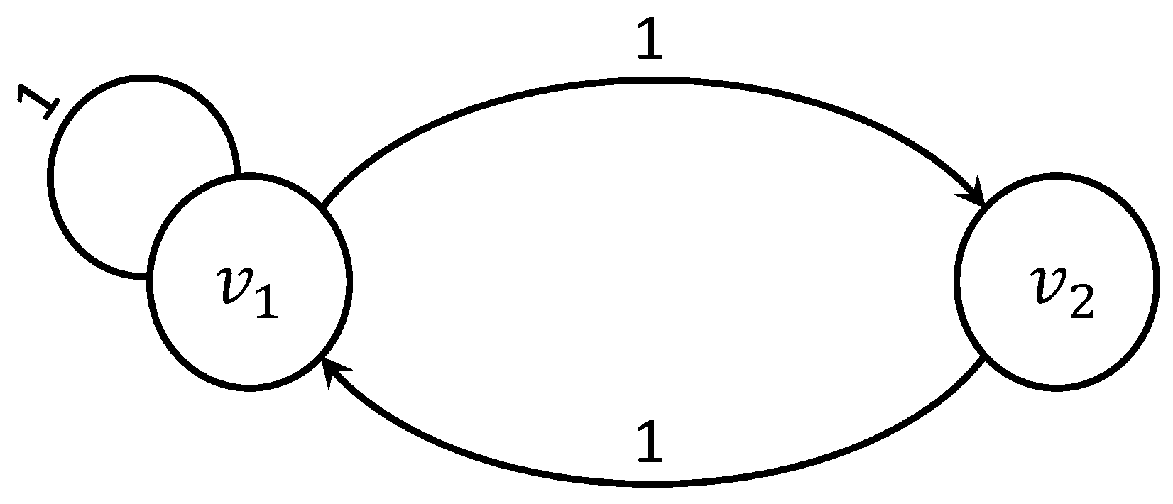
Example 1. Let the resource network be determined by the weighted graph with two vertices shown in Figure 1 with the throughput matrix R: The initial state vector is .
The functioning of this network is the following:
…
Thus, the stable state of the network is .
Let us analyze the law of changing states at the first steps and create the sequence of stochastic matrices defining a non-homogeneous Markov chain for its description. Consider the first vertex at the initial state: . This means that the vertex at time step sends some resource equal to 1 to each of two outgoing edges (one of them is a loop), according to Rule 1, and stores the rest of the resource, equal to 8, in itself. The vertex does not transfer anything, since . As a result, we have the state , but the same state would be obtained if the loop of the vertex had an arbitrary throughput in segment . If , then remains the same. If , then will change because the vertex will switch from Rule 1 to Rule 2 and will distribute its resource in the other way. Therefore, the value is a threshold value of the first vertex for the resource amount with a network topology determined by R.
Consider the new throughput matrix
:
As
, then
and
, so the vertex
uses Rule 2 and sends out its entire resource. The vertex
also uses Rule 2, which means that the next state
is obtained using Formula (
5) with the stochastic throughput matrix
:
At the next time step, to save the operation according Rule 2 (i.e., the equality
), the loop throughput of vertex
needs to be decreased by 1:
Then, the next state
can be calculated using the same formula with the new stochastic throughput matrix
:
As previously, the stable state of the resource network is .
is an equilibrium vector. However, the matrix itself is not a limit matrix of the (corresponding homogeneous) Markov chain. It is easy to verify this by considering its degrees.
However, , then and .
Matrix
is a limit of the degrees of a regular stochastic matrix. By definition, it consists of identical rows equal to the limit vector of the probability distribution. This vector, in turn, is a normalized equilibrium vector
, i.e., it is equal to
, and
By the property of the limit matrix of a homogeneous Markov chain:
Remark 2. The network operation in the example is very simple. The limit state is reached in one step. However, the behavior of resource networks with a large resource, in the general case, is rather complicated. The corresponding statements can be read in [28]; examples of the operation of networks with different topologies can be found in [33]. This example shows that the functioning of the resource network with the vertices having a large resource amount can be considered as the non-homogeneous Markov chain [
34].
In the general case, this transformation for the resource network with the initial state vector
and the throughput matrix
R can be written as follows:
Here,
, or
In the example above, the non-homogeneous Markov chain was strongly ergodic (see [
34,
35]):
Definition 7. A non-homogeneous Markov chain with stochastic matrices is called strongly ergodic ifwhere 1 is a column vector of n units and π is some probability vector. In general, if the limit state and the limit matrix exist, they can be found as
where
(
is some vector of the distribution of the resource
).
This equality holds for all strongly ergodic non-homogeneous Markov chains.
Let us turn to the study of strong ergodicity and the description of the limit characteristics of resource networks with the transient and regular components.
4. Study of Processes in Transient Components of Two-Component Resource Networks
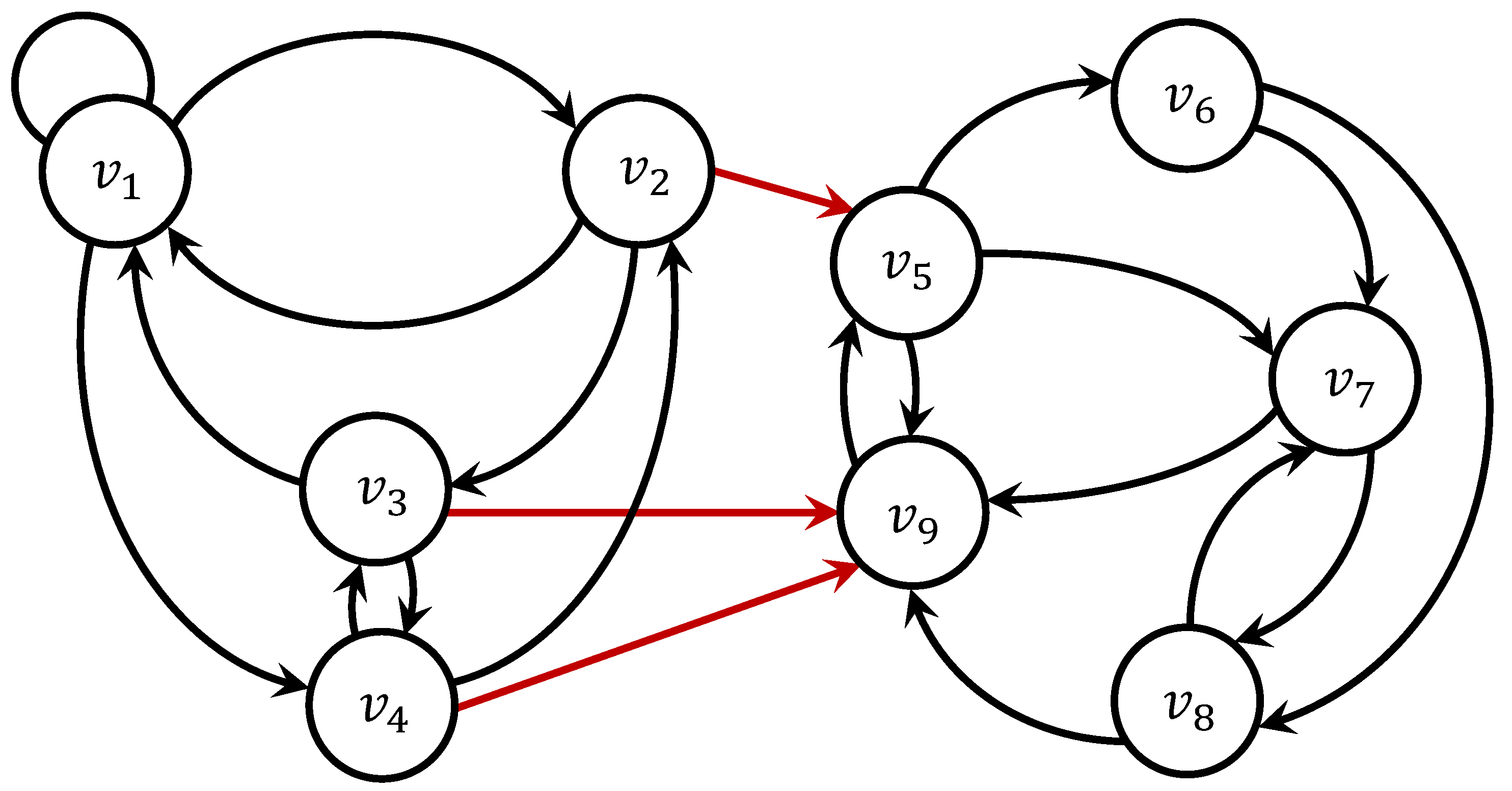
Consider a resource network with two strongly connected components, such that there are only edges from the first one (called the
transient component, with
vertices) to the second one (called
final, with
vertices). Let
n be the total number of vertices in the network (
Figure 2).
Theorem 1. There exists a finite time moment such that, for , all vertices of the transient component operate according to Rule 2.
Proof. We assumed there should always exist at least one vertex (say, ) in the transient component that has an edge to the final component. Otherwise the network graph is not even weakly connected. If so, we can analyze weakly connected components independently.
Suppose there is an excessive amount of resource in an arbitrary vertex of the transient component at time step t. Since the transient component is strongly connected, there exists a simple path . In that case, the resource equal to will be transferred from to at the time moment . This means vertex will contain at least resource. Next, at the moment , vertex will transfer at least resource to the vertex . In that case, at the moment , vertex will contain at least resource. If we continue this process, we will obtain that vertex will contain at least resource at the moment of time . Finally, at least resource will go to the final component at the moment (where is some edge from to some vertex in the final component). Therefore, if there was excessive resource in vertex at moment t, then, during time period (more precisely, ), at least resource will be transferred to the final component. It is important to note that depends on nothing but the fact that there was an excessive amount of resource in vertex .
Similar reasoning can be applied to any other vertex with excessive resource . Let us define . Then, the following holds: if, at some time moment t, an arbitrary vertex contained an excessive amount of resource, then by the time moment , at least resource will be transferred to the final component.
The proof now goes by contradiction: Suppose there is no moment from which the transient component operates according to Rule 2 all the time. In other words, suppose there exists an infinite sequence of time moments such that at least one vertex in the transient component contains excessive resource at each of these moments. Without loss of generality, assume that . Hence, at least resource will be transferred to the final component at each of the time intervals . The total amount of transferred resource is at least . The contradiction is now obvious since the resource network contains only a finite amount of resource by definition. □
Theorem 1 states that every possible resource distribution in the transient component sooner or later reduces to the linear case. The following theorem shows how the network behaves in the linear case.
Theorem 2. If the entire two-component network operates according to Rule 2, then the total amount of resource in the transient component tends to zero as time goes to infinity.
Proof. Let the network be defined by the matrix:
where
and
are nonzero square blocks corresponding to the edges of the transient and the final components, respectively;
is a rectangle block corresponding to the edges from the transient to the final component. The corresponding stochastic matrix is of the following form:
Whenever the network operates according to Rule 2, its next state is obtained according to Formula (
5).
If the network is operated according to Rule 2 for every
, then the following holds:
Passing to the limit as
(this limit always exists since the final component is regular):
Consider powers of matrix
:
and so on.
It follows from (
12) that the first
components of
are defined entirely by the first
columns of
. Therefore, only the left-side blocks of powers of
are of our interest. Since we can interpret
as part of the stochastic matrix corresponding to the transient component of a Markov chain, it is easy to prove then (using Theorem 3.1.1 of [
31]) that
It follows that, for each possible initial state
, such that the network operates according to Rule 2 forever, the limiting state will contain only zeros in the first
components (see (
12)). The statement of the theorem thus follows. □
The following theorem generalizes the two previous ones to the case of an arbitrary total resource amount in the network.
Theorem 3. In the two-component resource network, for any value and initial distribution of the network total resource, the total amount of resource in the transient component tends to zero as time goes to infinity.
Proof. Let the network be defined by the matrix:
and the resource is greater than the threshold value. Then, the resource distribution is described by a non-homogeneous Markov chain with a stochastic matrix:
The network operates according to the formula:
By Theorem 1, there is such a moment
, starting from which the transition component begins to function according to Rule 2. Then, for all
, the matrix
can be presented as matrix
, where
Thus, Formula (
17) can be written as follows:
In the second product, the block is constant; therefore, the first m columns tend to zero. Then, in the entire product, the first m columns tend to zero as time goes to infinity. □
Thus, for any total resource and any of its initial distribution in a two-component resource network, the entire resource will pass into the final component.
5. Some Properties of Stochastic Matrices
The above results can be generalized to arbitrary stochastic matrices, and some new properties can be derived. Theorem 2 implies the validity of the following theorem.
Theorem 4. For any rectangular stochastic matrix , where is a square block, is a rectangular block; if , the rectangular matrix is stochastic.
Proof. Let us relatea rectangular matrix to a square one as follows:
Consider the powers of the matrix
:
For
, there is
in the upper left block, as
is the block of stochastic matrix
. Furthermore, there is the sum of a infinite decreasing geometric progression with the denominator
in the upper right block:
Here, mentioning that
and
, the inverse matrix
exists always according to Theorem 1.11.1 in [
31]. The matrix
is stochastic; therefore, the matrix
is stochastic. Thus, if
, the matrix
is stochastic. □
The simple example demonstrates how Theorem 4 works.
Example 2. Consider the stochastic vector: Let us split it into two blocks, so that the first block is square dimensioned ,
Thus, according to the proven Theorem 4, the vector is also stochastic. Actually: An important generalization follows directly from Theorem 4.
Theorem 5. For any square stochastic matrix and for any arbitrary partition into blocks:where and are square blocks; if , the rectangular matrix is stochastic. 6. Limit States in Two-Component Resource Networks and the Strong Ergodicity of Non-Homogeneous Markov Chains
In
Section 4, it was established that, whatever the initial resource distribution is, all of the resource will be transferred to the final component in infinite time.
According to Proposition 2 and Corollary 2, if a resource network is regular, then in the case of a small resource, there exists a unique limit state that does not depend on the initial distribution.
In the case of a large resource, there also always exists a limit state, but if there are several attractor vertices (Definition 6), then the limit state might not be unique for every initial state. However, the limit state is always of the form (
9). What interests us is whether an analogy can be drawn with our case of a two-component network. The following theorems answer this question.
Suppose that the final component of the resource network is regular. Let
T (Formula (
7)) be the threshold value of the total resource
for the final component.
Theorem 6. If , then there exists a unique limit state that depends neither on the initial distribution of the total resource nor on blocks and of capacity matrix R.
Proof. The statement of the theorem means that there is no difference what the topology of the transient component is and what edges lead from the transient to the final component, if the resource amount is small.
If , it is assumed that there is a point of time from which the entire network operates according to Rule 2. Without loss of generality, suppose that the entire network operates according to Rule 2 from the first moment.
One can deduce from Equations (
13) and (
14) that an arbitrary power of
has the form:
where
According to Theorem 11.1 of [
32], there exists a limit
. Combining this fact with the statement of Theorem 2, we obtain that the limit must have the form
where
Multiplying the limit stochastic matrix by itself is idempotent (i.e.,
). That means the following:
The latter equation implies
Being a limit of the power of a regular stochastic matrix, consists of equal rows. Its rank is 1. Moreover, whenever any stochastic matrix is right-multiplied by , the result will also consist of the same rows. That being said, the matrix consists of the same rows as .
Suppose that
consists of rows
. Then,
has the form
It is obvious that
is of rank 1. It follows that the image of this linear operator (see Equation (
12)) is determined solely by the initial amount of resource
W.
The resource is a limit case for a small resource. By Proposition 2, for some initial states, two limit transitions are required to prove the theorem: the first one is for the transition of all vertices to Rule 2; then, the above reasoning is applied. □
Theorem 7. If , then for every initial state , there exists a limit state . If, additionally, the final component contains only one attractor vertex, then this limit state depends only on W, i.e., it depends neither on the initial distribution of the total resource and on blocks and of capacity matrix R.
Proof. In this case, it is assumed that there is a point of time from which at least one vertex of the network contains an excessive amount of resource.
It follows from Theorem 1 that there is a moment from which the entire transient component operates according to Rule 2. That means that all of the excessive resource is located in the final component (at least for sufficiently large moments of time). After this fact is established, the proof in the case
is made in analogy with the case
. The main difference is that
is not a limit of the powers of a single matrix, but a limit of the products of different matrices. However, it is known from the previous works [
28] that this limit of the products of matrices exists for every initial condition. In the case where there is only one attractor vertex in the final component, this limit of products depends only on
W. Thus, the statement of the theorem follows. □
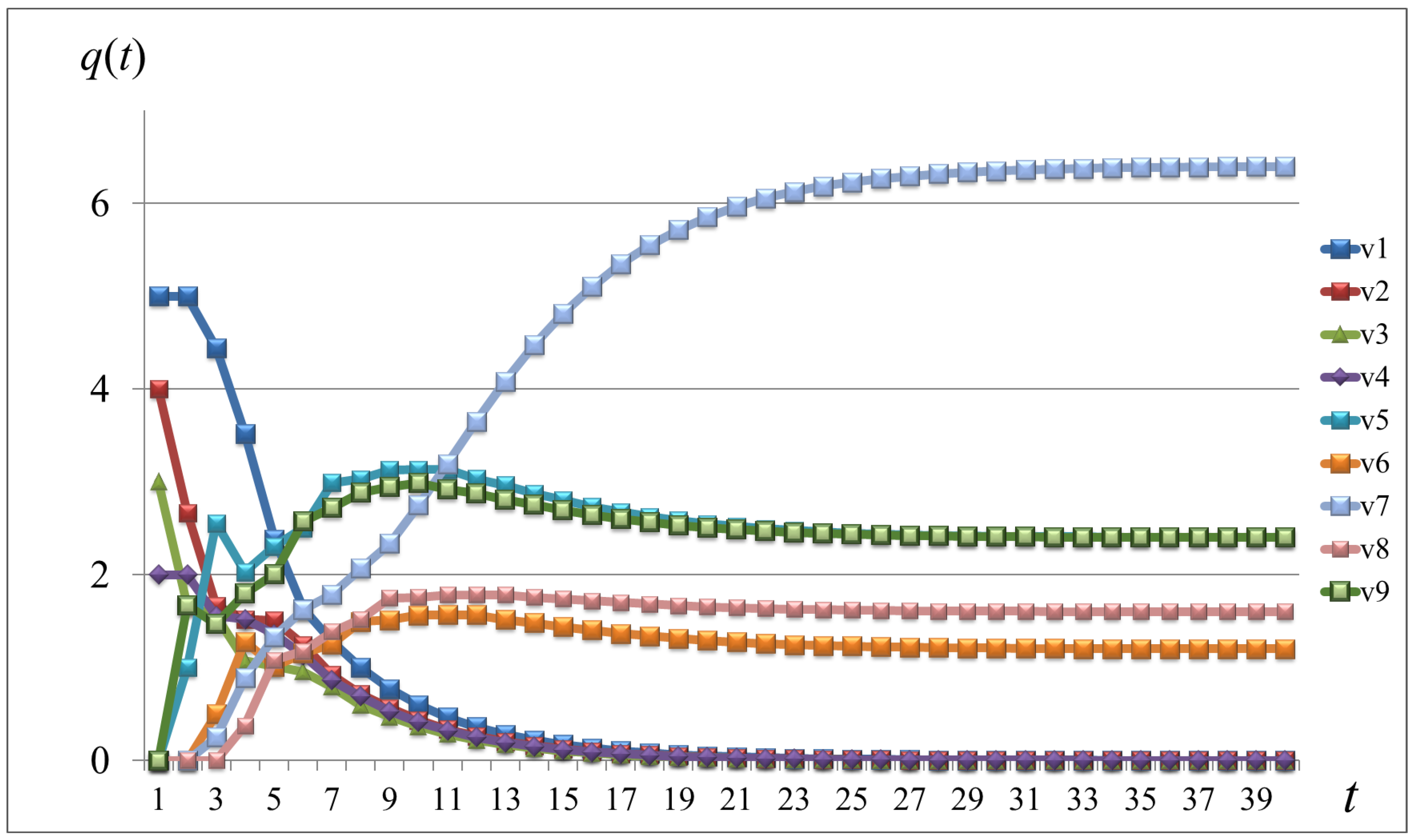
Example 3. Let us consider the two-component resource network shown in Figure 2. The edge weights are given by the matrix: Let and the initial state be given by vector . In this case, the entire resource is concentrated in the transient component.
The limit state is .
The functioning of the network is shown in Figure 3. On the graph, it can be seen how the resource flows from the transient component to the vertices of the final component.
If , then matrix sequences differ for different initial resource distributions . The infinite products of these matrices tend to the limit matrices (further, we omit the argument ).
Example 1 shows that, for at least some regular resource networks with
, there exist two stochastic matrices transforming the initial vector into the limit one:
It is easy to see that such matrices exist for any regular, as well as two-component networks and for any initial state .
The first matrix
is obtained from matrix
R defined by Formula (
10), where
; here,
are the components of a limit vector
. This matrix has different rows and is not a limit matrix. However, the limit matrix
is a limit of the powers of the stochastic matrix
.
Matrix is unique for every and consists of n normalized vectors .
Therefore, the following theorem is true.
Theorem 8. For a two-component resource network, if , then, for every initial state, the non-homogeneous Markov chain with stochastic matrices is strongly ergodic.
7. Discussion
The results presented in the article can be divided into three areas: two-component resource networks, stochastic matrices, and non-homogeneous Markov chains.
The main results concerning two-component resource networks were stated in the Theorems 6 and 7. It was proven that the two-component resource network with a regular final component is globally asymptotically stable, if
or
and there is a single attractor vertex. If there are several attractor vertices in a final component, the resource surplus is distributed among attractors (Formula (
9)) in a unique way described by Formula (
22).
The study of the behavior of two-component networks made it possible to prove a number of non-trivial statements about stochastic matrices, as well as about non-homogeneous Markov chains.
In our opinion, Theorems 4–6 deserve special attention, since they formulate the interesting properties of stochastic matrices. These properties are universal and applicable to any stochastic matrices, without reference to the resource network model.
Theorem 8 states that the non-homogeneous Markov chain describing the operation of the two-component resource network with a regular final component for is strongly ergodic. This implies that the non-homogeneous Markov chain describing the regular resource network with is definitely strongly ergodic.
The non-homogeneous Markov chain corresponding to the given network and given initial distribution of resource
is defined by Formula (
10). Two matrices that transform the initial distribution into the limit distribution are presented in Formula (
22), and their relationship is in Formula (
23).
In the future, we plan to obtain an analytical formula for resource allocation among attractors in the limit state for a network with several attractors and . This problem still remains open.
8. Conclusions
The resource network model is described by very simple operation rules; however, it is capable of generating complex behavior. Moreover, the network turned out to be a good tool for studying the properties of stochastic matrices and Markov chains.
In our team, two extensions of resource networks were proposed and studied: a network with the capacity limitations of attractor vertices and a network with greedy vertices [
28].
Based on the resource network defined by a regular grid, a model of the distribution of pollutants on the surface of a reservoir was developed [
36].
In our future research, we plan to study new modifications of resource networks, such as networks with dynamic throughputs. Using such a model, it will be possible to search for bottlenecks in the distribution of traffic in networks of various kinds—from transport to telecommunications.


