Article

Comparative Study on Lower-Middle-, Upper-Middle-, and Higher-Income Economies of ASEAN for Fiscal and Current Account Deficits: A Panel Econometric Analysis

1
Department of Management and Humanities, Universiti Teknologi PETRONAS, Seri Iskandar 32610, Malaysia
2
Department of Economics, Kohat University of Science and Technology, Kohat 26000, Pakistan
3
Institute of Management Sciences (IM|Sciences), Peshawar 25000, Pakistan
*
Author to whom correspondence should be addressed.
Mathematics 2022, 10(18), 3259; https://doi.org/10.3390/math10183259
Submission received: 13 July 2022 / Revised: 12 August 2022 / Accepted: 17 August 2022 / Published: 7 September 2022

Abstract

:
For the last three decades, ASEAN has been facing a persistent fiscal deficit. However, the impact of fiscal deficit on the current account deficit in the sub-groups of ASEAN is still unknown. This study aims to investigate the impact of fiscal deficit on current account deficit and their relationship among the three sub-groups of ASEAN which are based on gross national income (GNI), i.e., lower-middle-, upper-middle-, and higher-income countries. The analysis covers the panel data collected over the span of the last three decades (1990–2020) for ten Southeast Asian nations (ASEAN). The analyses incorporate the panel methodology for data analysis such as panel unit root for checking data stationarity, cointegration testing, panel autoregressive distributed lag (PARDL) for short- and long-run analysis, cointegration regression (fully modified and dynamic ordinary least squares) for significance, the panel Dumitrescu and Hurlin Granger causality test for examining causal relationships in tested variables, and stability diagnostics and CUMSUM and CUSUMSQ techniques for structural breaks and coefficient stability in the model. In lower-middle-income economies (LMIE), results indicate the existence of a unidirectional causal relationship from the current account deficit (CAD) to the fiscal deficit (FD), suggesting a reverse causal relationship from CAD to FD. In the long run, FD does not significantly induce CAD, while real interest rate (RIR) and exchange rate (EXC) influence CAD. In upper-middle-income economies (UMIE), results specify that there is no causality between FD and CAD. The RIR, EXC, and FD are significant to CAD in the long run. In higher-income economies (HIE), RIR and FD have an influence on CAD in the long run period. Moreover, from CAD to FD, a unidirectional causal association exists, and likewise for LMIE. This is a reverse causal relationship from CAD to the FD, supporting the current account targeting hypothesis (CATH) in both the LMIE and HIE groups. This study recommends that the LMIE and HIE groups can use the fiscal deficit as a tool to eliminate the unfavorable current account position. Policymakers can target EXC and RIR to stabilize CAD in long run. In UMIE and HIE, policymakers must consider FD alarming, as it can induce CAD in the long run. The RIR can be the targeted factor in the sub-groups of ASEAN.

1. Introduction

In the international financial system, current account and fiscal deficit relationships have raised many questions. These questions are debatable among policymakers, practitioners, and academic departments. The association between fiscal deficit and current account deficit is based on the causal direction between them. When a fiscal deficit prevails in any economy, it causes a current account deficit, which is called the twin deficit hypothesis [1]. In vast literature, the causal association between current accounts and fiscal deficit is contentious. After facing a fiscal deficit, economies utilize expansionary fiscal policies, which can make the current account balance unfavorable [2]. This imbalance disrupts economic activities.
This study focuses on the association of southeast Asia income sub-groups. These are lower-middle-income countries, upper-middle-income countries, and higher-income countries. The main reason for this focus is the dynamic growth of this region. Economists and practitioners call this region an “economic powerhouse”. ASEAN is the world’s most competitive emerging economic region. The Asian Financial Crisis (AFC ’96) and Global Financial Crisis (GFC ’07) had a stroke on Southeast Asia. In the early 1990s, ASEAN hardly had control over the aggressive influences of unfavorable trade balance and, at the same time, the Asian Financial Crisis (AFC) hit Southeast Asia. For Southeast Asia, export trade is the primary growth engine as the main source of income. In the 1990s, ASEAN recorded huge fiscal and current account deficits. The big matter of concern for policymakers and practitioners was the random variations in these deficits. During the global financial crisis, the annual growth rate of ASEAN declined [3,4]. Mostly, member nations lost their currency values, which led to making the trade balance unfavorable. After the global financial crisis, recently the world has been facing the COVID-19 pandemic, which also affected the ASEAN region in Asia. The governments of member nations have launched their emergency support packages. These emergency packages include food subsidies, wage subsidies, tax rebates, cash payments, grants, utility bill subsidies, etc. Emergency packages and health expenditures are making the fiscal deficit worse.
The World Bank has grouped the worldwide economies based on gross national income (GNI) per capita into four income groups. These income groups are high-income economies, upper-middle-income economies, lower-middle-income economies, and low-income groups of economies. Recently, in the year 2020, the low-income countries were defined with a GNI per capita of USD 1036, lower-middle-income with USD 1036 to USD 4045, and upper-middle-income with USD 4046 to USD 12535, whereas the high-income threshold was above USD 12,535. The ASEAN’s GNI per capita categories are shown in Figure 1.
In ASEAN, lower-middle-income economies (LMIE) include the Philippines, Lao PDR, Vietnam, Myanmar, and Cambodia. Upper-middle-income economies (UMIE) include Malaysia, Indonesia, and Thailand. Higher-income economies (HIE) include Singapore and Brunei Darussalam. From the year 2016 onwards, the lower-income economies of ASEAN have improved their economies and reached lower-middle-income countries. A large number of studies have investigated ASEAN [5,6,7,8,9,10,11,12,13,14,15]. However, none of these studies reported the twin deficit hypothesis in ASEAN’s income sub-groups. It will be worth investigating the impact of fiscal deficit on the current account deficit in three panels of ASEAN’s income sub-groups.
As suggested by [16], to validate the fiscal deficit, it is expedient to ensure its connection with other interconnected financial factors. This study considers one of those interconnected factors, i.e., current account balance. In ASEAN, before the Asian Financial Crisis (AFC), the current account deficit was less volatile and persistent in nature, while the fiscal balance was already in deficit even before the AFC. After the AFC, the 1999–2002 fiscal deficit turned worse and influenced the current account deficit. The current account balance turned much worse in the Global Financial Crisis (GFC) due to the worst fiscal balance. Figure 2 and Figure 3 show the trends of fiscal and current account balances, respectively.
As reported by the Finance Ministry of Malaysia, the fiscal balance in the first five months of 2018 was in a deficit of about MYR 35 billion. At the same time, the current account deficit was about MYR 17.1 billion. In 2019, the fiscal position was improved by MYR 14 billion. The government of Malaysia has shrunk its current account deficit by MYR 16.1 billion (see Table 1). In ASEAN, each member nation is a small open economy, and its exports are significantly influenced by global factors. For instance, the Asian Financial Crisis in 1997 and the Global Financial Crisis in 2007 hit ASEAN’s exports sector. The negative effects of unfavorable trade were extensive, leading to slowing down growth, worsening the current accounts, and generating inflationary pressures. Recently, in COVID-19, according to the Asian Development Bank, each member of ASEAN spent a huge amount of money to support COVID-19 expenditures; see Table 2. The previous trends of fiscal and current account deficits in 1997, 2007, and 2020 show that fiscal deficit in ASEAN is influential to current account deficit. The current account balance is the reflection of savings and investments. If the economy utilizes more than its savings, then a current account deficit can occur (See Figure 4). In ASEAN-5, when investments are high the current account balance is in deficit, while when investment is low the current account balance is in surplus. The current account balance is a mirror of the economy’s investment and consumption. Vietnam, Malaysia, and Singapore spent large amounts to support COVID-19. ASEAN was facing a fiscal deficit even before COVID-19. Moreover, recently, the fiscal deficit has gotten much worse due to high health expenditures. It is worth investigating the consequence of fiscal deficit, i.e., the current account balance.
The association between fiscal and current account deficits is defined differently by different schools of thought. One of the schools of thought is the Keynesian school of thought. According to Keynesian macroeconomics, Mundell–Fleming’s theory states that a fiscal deficit can cause a current account deficit and generate a double/twin deficit in the economy. The fiscal deficit leads to an increase in the real interest rate. It will encourage the capital inflow and appreciation of the exchange rate, which will lead to the current account deficit [17]. In general, the fiscal deficit can influence the current account deficit in many ways, as it has short-run and long-run effects on the exchange rate; see Figure 5.
The connection between fiscal policy and current account balance has short-run and long-run impacts on the exchange rate. Expansionary fiscal policy has a short-run influence on the exchange rate through the channel of interest rate and capital inflows, which leads to the appreciation of the exchange rate, while in the long run, after expansionary fiscal policy, government debt builds up. The first way to finance this debt is by the central bank (the domestic source of financing) monetizing the debt. The second way is to put restrictions on fiscal stance. These ways can depreciate the currency and recover the current account deficit. Therefore, this study considers the long-run and short-run impacts of expansionary fiscal policy on the exchange rate, which leads to a change in the current account balance. Previous studies such as [12,18,19] investigated the twin deficit hypothesis in ASEAN with different perspectives. The current study validates the fiscal deficit through one of its interconnected factors, the current account balance. The trends of fiscal deficit in overall ASEAN are in some way different from the trends in the sub-groups of ASEAN. Hence, for policy implications, it would be beneficial for the policy think tanks to target the individual groups of ASEAN for implementing a fiscal policy according to its trend in each sub-group. Consequently, it is accountable and worth investigating the following: “Is fiscal deficit influencing the current account balance in ASEAN’s income sub-groups?”. This study examines the panels of three sub-groups, i.e., lower-middle-income economies (LMIE), upper-middle-income economies (UMIE), and higher-income economies (HIE). The study aims to explore the twin deficit hypothesis (the impact of fiscal deficit on current account deficit and fiscal deficit does cause current account deficit). For this purpose, this study has certain objectives. The first objective of this study is to investigate the impact of the fiscal deficit on the current account deficit in the short run and long run. The second objective is to evaluate the causal association between the fiscal and current account deficits. The third objective is to examine the behaviors of exchange rate and interest rate in ASEAN’s income sub-groups.

2. Literature Review

In theory, there are four possible outcomes regarding the causality between fiscal and current account deficits, as shown in Table 3.
There are few studies that have analyzed the ASEAN twin deficit hypothesis, i.e., Lau, Mansor, and Puah [26], Magazzino [15], Shastri, et al. [18], and Baharumshah and colleagues [19]. Lau et al. [26] investigated the relationship between fiscal and current account deficits in Indonesia, Malaysia, Thailand, and the Philippines. After utilizing unit root, cointegration, and Granger causality, the study found that there is a two-way/bidirectional relationship between fiscal and current account deficits in the Philippines. CATH is supported in Indonesia, and the twin deficit hypothesis is confirmed in Malaysia and Thailand. Magazzino [15] examined the twin deficit hypothesis in ASEAN-10 and ASEAN-6. The study utilized the panel unit root [27], panel cointegration test [28], and panel Granger causality technique and found that Ricardian equivalence theory prevails in Southeast Asia. In other words, there is no causality between fiscal and current account deficits in ASEAN. Shastri et al. [18] investigated the causal relationship between fiscal and current account deficits in South Asia and Southeast Asia. The study utilized panel cointegration and Dumitrescu and Hurlin’s (DH) panel causality. The results showed that there is a bidirectional/two-way causal relationship between fiscal and current account deficits. Baharumshah and colleagues [19] observed fiscal and current account deficits in ASEAN-5 and concluded that Malaysia, Thailand, and the Philippines support the twin deficit hypothesis. Moreover, an increase in government expenditures completely crowds out private investment. Marimuthu et al. [29,30] investigated the twin deficit hypothesis in ASEAN-10 by utilizing Panel ARDL, panel cointegration regression (fully modified ordinary least square and dynamic ordinary least square) Dumitrescu and Hurlin (DH) [31] for panel causality. The results indicate that in ASEAN-10 the current account targeting hypothesis is satisfied. The real interest rate is influential on both deficits as a moderator.
In a recent empirical review, most of the studies were conducted on ASEAN-10, ASEAN-5, or individual members. According to the World Bank classification based on GNI, ASEAN is classified into three groups: LMIE, UMIE, and HIE. These groups are different from each other on the basis of GNI, which is the best indicator of living standards. This study considers the comparative analysis between these three groups of ASEAN, as there are different trends in fiscal and current account balances (see Figure 2). However, policymakers can target the specific group of ASEAN rather than the overall ASEAN for the consequence of fiscal deficit which has been experienced in ASEAN in past trends during financial crises. Therefore, it is accountable and worth investigating the following: “Does fiscal deficit influence the current account balance in the three groups of ASEAN?”.
In this way, the policymakers can implement different policy measures in each group according to its fiscal situation. In the next section, this study presents the methodology for this analysis.

3. Materials and Methods

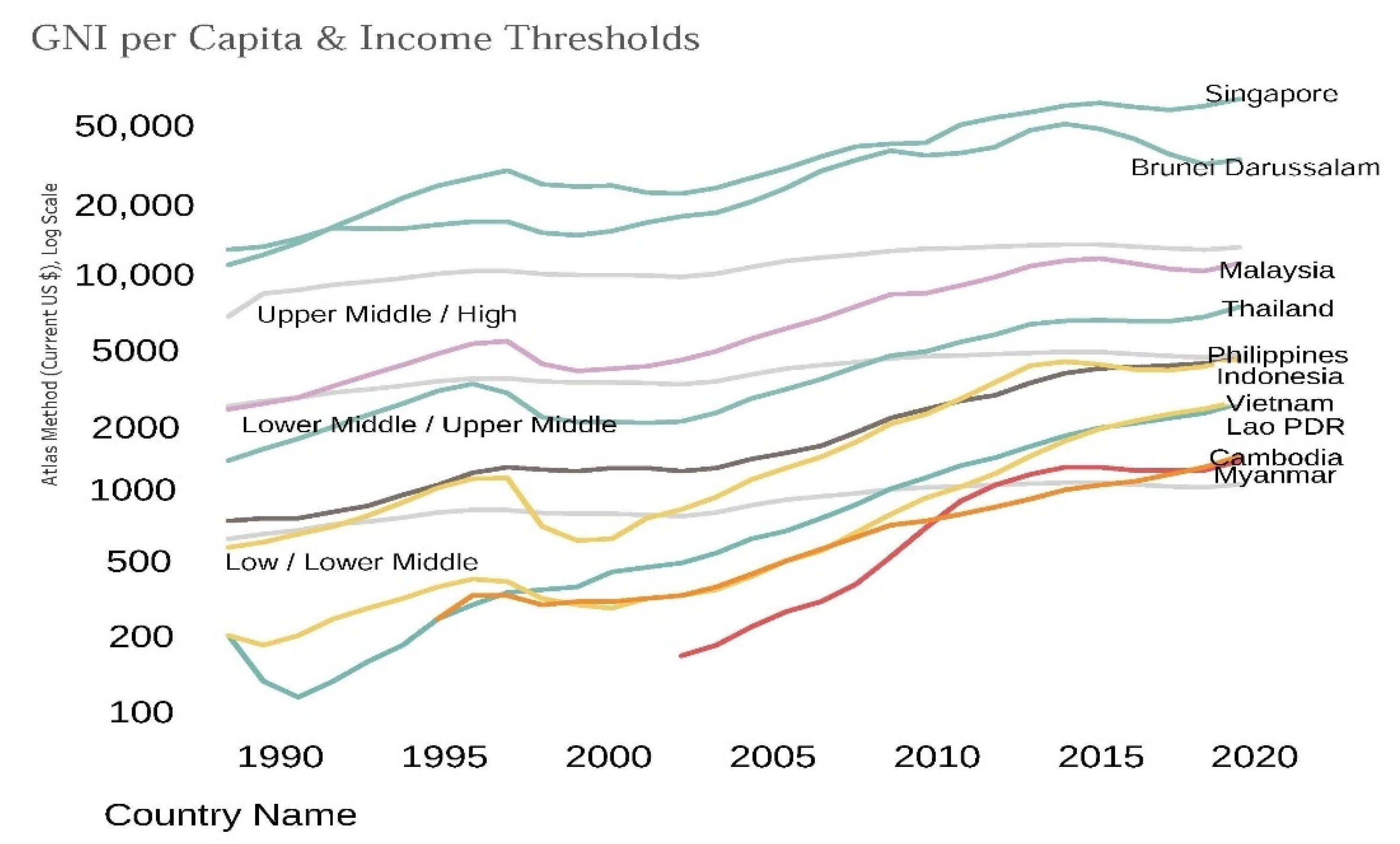
3.1. Data and Variables

This study is a comparative study and consistent with causal research methods. This study compares the three income sub-groups of ASEAN in the context of the twin deficit hypothesis. These income sub-groups are lower-middle-income-, upper-middle-income-, and higher-income economies. To carry out this investigation, this study follows a quantitative approach and utilizes panel data methodology for ASEAN income sub-groups. The data for this investigation have an annual frequency, from 1990 to 2020. This time span selection is based on data availability and collected from authentic sources from the World Bank Database (WBD) and Asian Development Bank (ADB). This study utilizes three-panel sets, a panel for each sub-group (LMIE, UMIE, and HIE). Before investigating the data, it is important to scrub and transform the dataset to avoid any roughness in the data. The data scrubbing process includes removing and fixing the corrupted and duplicated data, especially when combining different sources of data. Further, irrelevant observations are also removed which do not fit into the problem, for example, unwanted outliers. Missing data cannot be ignored during the data scrubbing process, as most of the algorithms do not accept missing values. Therefore, in the dataset, there are one or two missing values at random (MAR), which are handled by using imputation through the mean. In data transformation, the log form of each variable is taken. Few variables, for instance, fiscal deficit (FD) and inflation, are already in percentages. Hence, this study utilizes the data after the scrubbing and transformation process. LMIE includes five economies, i.e., the Philippines, Lao PDR, Vietnam, Myanmar, and Cambodia. Upper-middle-income economies (UMIE) include three economies, Malaysia, Indonesia, and Thailand. Higher-income economies (HIE) include Singapore and Brunei Darussalam. Therefore, there are 31 annual observations for each country. The LMIE panel has 151 observations and 5 cross-sections, the UMIE has 93 observations and 3 cross-sections, and the HIE has 62 observations and 2 cross-sections. This study uses Econometric Views (EViews) as an econometric tool to obtain the output. For the mentioned panel datasets, the study utilizes econometric techniques, i.e., panel autoregressive distributed lag (ARDL) and panel cointegration regression (FMOLS and DOLS). These techniques pass through many diagnostic issues for instance endogeneity, heteroscedasticity, serial correlation, etc.
The variables employed in the analysis are defined below:
Current account balance: The current account balance refers to the situation where exports are equal to imports. This balance can be in the form of a surplus or deficit. The current account balance would be in deficit when imports are greater than exports, while the situation when exports are greater than imports relatively is known as surplus. From 1990 to 2020, most of the years, ASEAN faced a deficit. This study utilizes the current account balance as a consequence of fiscal deficit.
Fiscal balance: Fiscal balance refers to the situation where government expenditures are equal to government revenues. This balance indicates the amount the government receives in revenues from taxes/non-tax resources and spends on government expenditures, for instance, developmental expenditures, such as infrastructure, schools, hospitals, government buildings, etc. This balance can be negative when expenditures exceed revenues, and this is called a fiscal deficit. Likewise, when revenues exceed expenditures, this is known as a surplus. From 1990 to 2020, in most of the years, ASEAN faced a fiscal deficit.
Official exchange rate: The official exchange rate is officially set by government authoritative institutions. This study utilizes the official exchange rate as recommended by the Mundell–Fleming model. It has a significant influence on the trade balance, as investigated by previous studies [32,33,34].
Real interest rate: The real interest rate is adjusted for inflation, and it is measured by the GDP deflator. It plays an essential role in the transmission mechanism of the twin deficit hypothesis referred to by the Mundell–Fleming model.
Gross domestic product: The final value of goods and services produced within a country is known as GDP. This study utilizes GDP as an exogenous factor in the Mundell–Fleming model to avoid any misspecification error and spurious causal effect in the model. The list of variables with data sources and units is given in Table 4.

3.2. Empirical Model

The objective of this study is to investigate the causal association between the fiscal and current account deficits in each income sub-group of ASEAN. Mundell–Fleming’s model is proposed in this study, based on Keynesian macroeconomics. This model states that the fiscal deficit (increase in govt. ex.) can increase the real interest rate (RIR) which encourages the capital inflow and appreciation of the currency, which leads to a current account deficit. This study proposes an empirical model for three income sub-groups, as current account deficit is a function of fiscal deficit, official exchange rate, real interest rate, and GDP. The functional form of this model is given below.
C A B = f F B ,   E X C ,   R I R ,   G D P
The mathematical expression of the model is
C A B i t = α 0 + β 1 F B i t + β 2 E X C i t + β 3 R I R i t + β 4 G D P i t + ε i t
In Equation (2) above, CAB refers to the current account balance, FB is the fiscal balance, EXC is the official exchange rate, RIR is the real interest rate, and GDP is the gross domestic product. To analyze this model, this study employs panel econometric techniques, including the panel unit root test, panel cointegration ARDL, cointegration regression, and the DH panel Granger causality test.

3.2.1. Panel Unit Root Test

The panel time series data from 1990 to 2020 for each income sub-group (LMIE, UMIE, HIE) are assumed to be non-stationary. Therefore, to test the stationarity, the study utilizes Levin, Lin, and Chu (LLC) [35] and Pesaran and Shin (IPS) [36]. LLC assumes a collective unit root process and has the null hypothesis that each panel time series in the panel contains a unit root [35] and the IPS method assumes each cross-section unit root process, as the unit root coefficient may vary across each cross-section of panel [36]. Generally, the IPS method is not restrictive in nature, as it assumes the heterogeneous coefficients of a unit root. The null hypothesis for IPS is that all cross-sections have a unit root. The LLC test assumes that the error term is independent across the cross-sections and has constant variance. In Baltagi [37], it is suggested that the LLC test shows satisfactory performance in the data with cross-sections greater than 5, and observations lie between 10 and 250. After performing panel unit root techniques, the next step is finding cointegration.

3.2.2. Panel Cointegration Autoregressive Distributed Lag (ARDL)

To further analyze the econometric model, the long-run association among the variables is important. The panel ARDL has the advantage of being utilized on the stationary/non-stationary or mixed results of a unit root. In recent studies, panel ARDL is preferred over the traditional cointegration techniques. Hall and Asteriou [38] suggested that panel ARDL controls the endogeneity problem of independent variables. Furthermore, panel ARDL is beneficial to disclose the long-run and short-run dynamics of the model [39]. The panel ARDL model based on the econometric model of this study is given below.
k = 1 K Δ C A D i t = β o + β 1 i k = 1 K Δ F D t k + β 2 i G D P i + β 3 i k = 1 K Δ E X C t k + β 4 i k = 1 K Δ I R t k + θ 1 F D t 1 + θ 2 G D P i + θ 3 E X C t 1 + θ 4 I R t 1 + ε i t
k presents the number of lags, t is time, and i t shows the cross-section at time t. The hypotheses for a long-run relationship among tested variables are given below.
H 0 : θ 1 = θ 2 = θ 3 = θ 4 = 0 H 1 :   θ i 0
The null hypothesis for the cointegration relationship is “there is no cointegration” and the alternative hypothesis is “there is cointegration and at least one coefficient ( θ ) is not zero”. The long run and short run equations are extracted from the panel ARDL model (Equation (3)).
k = 1 K C A D i t = α o + α 1 i k = 1 K F D t k + α 2 i k = 1 K E X C t k + α 3 i k = 1 K I R t k + ε i t
k = 1 K Δ C A D i t = β o + β 1 i k = 1 K Δ F D t k + β 2 i G D P + β 3 i k = 1 K Δ E X C t k + β 4 i k = 1 K Δ I R t k + ν E C T i t + ε i t
Equation (4) is for the long-run relationship. Equation (4) refers to short-run dynamics. Coefficients β 1 i ,   β 2 i ,   β 3 i ,   β 4 i refer to the values of the t k period. The ECT term in Equation (5) indicates the error correction term which presents the adjustments towards long-run equilibrium. The ECT equation is given below.
E C T i t = C A D i t α o α 1 i k = 1 K F D t k α 3 i k = 1 K E X C t k α 4 i k = 1 K I R t k

3.2.3. Panel Cointegration Regression

In panel data analysis, after observing the long-run and short-run dynamics, it is important to re-estimate the model for cointegration regression. Cointegration regression is known to generate efficient estimators, as argued by Kao and Chiang [40]. Efficient techniques for cointegration are fully modified ordinary least square (FMOLS) and dynamic ordinary least square (DOLS). These two techniques are supportive in dealing with endogeneity and serial correlation issues. Rahman et al. [41] proposed utilizing DOLS, as it performs well relative to FMOLS and OLS. Arize et al. [42,43] mentioned that DOLS can provide unbiased results by adding leads and lags in the model and utilizing the white heteroscedasticity standard errors to avoid heteroscedasticity in the panel model.

3.2.4. Dumitrescu and Hurlin (DH) Granger Panel Causality Test

The main objective of this study is to investigate the causal association between fiscal and current account deficits. For examining causal effects, this study employs the DH Granger causality test [31], which is best for panel data. This test is preferred to the other traditional Granger causality tests because it is suitable for unbalanced data and it takes into account the heterogeneous nature of panel data and also cross-sectional dependence. This technique has two estimations: first, it estimates the heterogeneous nature of the panel econometric model, and second, it estimates the heterogeneous nature of the causal relationship. The DH causality test assumes the adjusted Wald is good and can be utilized to investigate the panel causal association among the tested variables. This study has four causal models.
C A D i t = γ 0 + γ 1 i j = 1 k F D t j + γ 2 i j = 1 k E X C t j + γ 3 i j = 1 k I R t j + μ i t
F D i t = γ 0 + γ 1 i j = 1 k C A D t j + γ 2 i j = 1 k E X C t j + γ 3 i j = 1 k I R t j + μ i t
E X C i t = γ 0 + γ 1 i j = 1 k C A D t j + γ 2 i j = 1 k F D t j + γ 3 i j = 1 k I R t j + μ i t
I R i t = γ 0 + γ 1 i j = 1 k C A D t j + γ 2 i j = 1 k F D t j + γ 3 i j = 1 k E X C t j + μ i t
The null hypothesis for the DH causality test is “there is no causal homogenous causal relationship”, which is called homogenous non-causality (HNC). Against the null hypothesis, this technique has two alternate hypotheses: the first is that there is a heterogeneous causal relationship but not in all cross-sections, and the second is that there is causality in all cross-sections.
H 0 = γ 1 i = γ 2 i = γ 3 i = 0 i = 1 , 2 , , N H A 1 = γ 1 i = γ 2 i = γ 3 i = 0 i = 1 , 2 , , N 1 , N 1 < N H A 2 = γ 1 i γ 2 i γ 3 i 0 i = N 1 + 1 , N 1 + 2 , , N

3.2.5. Diagnostic Checks

Endogeneity

Endogeneity issues in panel data emerge due to the existence of omitted variables, misspecification, and simultaneity between dependent and independent variables. This study utilizes the Hausman test to detect the misspecification, the likelihood test to detect the omitted variable, and panel ARDL which passes through many diagnostics such as serial correlations and endogeneity issues.

Heteroscedasticity

In panel data with N < T (N refers to numbers of cross-sections and T refers to time series), the dataset may face heterogeneity issues, which can be observed and unobserved. This issue arises due to variance dynamics. This study is dealing with heterogeneity issues with dynamic ordinary least squares and fully modified least squares (DOLS and FMOLS). FMOLS passes through the diagnostics of autocorrelations and heterogeneity by clustering the stand errors. DOLS deals with heterogeneity by utilizing the white heteroscedasticity standard error [44].

3.2.6. Stability Checks

Different economic and political instability shocks can generate structural changes in an economy. In particular, in panel financial data, it is important to check stability in the model [45,46]. For this purpose, the study considers change point detection, which means the specific time when the behavior of the data changes. Change point detection for each cross-section is possible in panel data. This study utilizes regression-based methods for change point detection. These are the cumulative sum and cumulative sum of squares (CUSUM and CUSUMSQ). Recursive estimates are to be employed in this method. CUSUM is utilized to detect the structural change in the model, while CUSUMSQ is used to ensure the stability of the coefficients in the model.

4. Empirical Findings

4.1. Findings from Panel Unit Root Testing

In the regression testing of panel data, it is important to check data stationarity. This study considers two-panel unit root testing: that of Levin et al. [35] for the collective unit root and that of Im et al. [36] for the individual unit root. To avoid a high level of autoregression, the AIC criterion is used to identify the number of lags. GDP, CAD, EXC, FD, and RIR are tested for a unit root in each panel (LMIE, UMIE, and HIE). In LMIE, the GDP, FD, CD, and EXC are stationary at level first and integrated at one order I(1), while RIR is stationary at level and integrated at I(0). In UMIE, the GDP, FD, and EXC are stationary at the first difference and integrated at I(1), whereas RIR and CAD are stationary at level. In HIE, the GDP, CAD, FD, and EXC are stationary at first difference, while RIR is stationary at level. The computed results for panel unit root for three panels are presented in Table 5, Table 6 and Table 7.

4.2. Fixed/Random Effects for Panel Data

In order to select the best model for the panel data, tests are needed to be conducted systematically, such as a Chow test (redundant fixed effects test), Lagrange multiplier test (omitted random effects test), and Hausman test (correlated random effects test). In Table 8, systematic findings reveal that, in each income sub-group of ASEAN, the random effect model is more efficient (it has a small asymptotic variance). Cross-sectional independence is also supported in each group.
After concluding the random effects in income sub-group in Table 8. Table 9, shows the significance level of each tested variable in standard panel regression, which is the estimation of generalized least square. The results indicate that RIR significantly influences CAD in LMIE and HIE, while RIR and EXC both significantly affect CAD in UMIE. A fiscal deficit is not creating another deficit, which is the current account deficit. After estimating the EGLS for all the panels, this study analyzes the model through panel ARDL. Panel ARDL is a well-behaved technique that passes diagnostic tests as well, for instance, serial correlation and endogeneity issues in the model. Further, PARDL is exploring the long-run and short-run dynamics between the tested variables. The results of panel ARDL for all the panels are in Table 10, Table 11 and Table 12.

4.3. Findings of Panel ARDL for Three Sub-Groups

After panel unit root tests on three panels, this study utilizes panel ARDL for investigating the short-run and long-run dynamics. Panel ARDL covers the lack of traditional cointegration tests, as discussed by Pedroni [47]. It is suitable to deal with the endogeneity problem of independent variables [48]. The null hypothesis for panel ARDL is “there is no cointegration between variables”. In panel LMIE, the auto-adjusted model is selected at lag 2, ARDL (2,2,2,2). ARDL estimates long-run and short-run dynamics simultaneously. In the long-run equation of LMIE, FD is not significant to CAD, while EXC and RIR are highly significant and influence CAD, as shown in Table 10. The exchange rate is inversely related to CAD, as a one percent increase in the exchange rate can bring a 0.14% decrease in CAD in the long run. In the short-run equation, the ECT term is highly significant. About 78 percent convergence is possible annually to the long-run equilibrium. The lag values of the tested variables are insignificant to CAD in the short run.
In the panel ARDL of UMIE, as shown in Table 11, RIR is significant to CAD and has a long-run relationship, while EXC and FD are insignificant to CAD. The ECT term is highly significant and shows a 69 percent convergence to the long-run equilibrium annually. A two-year lag value of EXC is significant to CAD in the short run. Similarly, a two-year lag value of FD is significant and has a short-run relationship with CAD. The lag values of RIR and EXC are not significant and have no short-run relationship with the current account deficit.
In HIE, as shown in Table 12, RIR and FD are significant to CAD and have a long-run relationship. A one percent increase in FD can generate a 0.02 percent increase in current account deficit (CAD). A one percent increase in real interest rate creates a 0.006 percent increase in CAD. The exchange rate is insignificant in HIC. In short-run dynamics, the error correction term is significant and converges to long-run equilibrium by 98 percent annually. The one-year lag value of RIR is significant in the short run, while the two-year lag value of fiscal deficit is significant to CAD in the short run.

4.4. Findings of Panel Cointegration Regression

Cointegration regression is helpful to generate the normally distributed efficient estimators. In panel data analysis, it is important to re-estimate the model to analyze the magnitudes/sensitivities of coefficients. Efficient techniques for panel cointegration regression are fully modified ordinary least squares (FMOLS) and dynamic ordinary least squares (DOLS). This study utilizes both techniques. FMOLS and DOLS support avoiding endogeneity and serial correlation issues. Previous studies such as [42,43] have recommended utilizing DOLS because it performs well relative to OLS and FMOLS. DOLS resolves the endogeneity problem by adding leads and lags in the model and it uses the white heteroscedasticity stand errors to cover up the heteroscedasticity problem in the model. The FMOLS and DOLS results for each group, i.e., LMIE, UMIE, and HIE, are presented in the sub-sections as follows.
The cointegration regression results for LMIE are presented in Table 13. The results show that RIR is significant in FMOLS and DOLS. The RIR coefficient is much more sensitive in FMOLS relative to the coefficient in DOLS. EXC is significant at 4 percent in FMOLS, while, in DOLS, EXC does not significantly influence CAD. In FMOLS, the coefficient of EXC is more sensitive at 1.93, greater than unity. A one percent increase in EXC can bring a 1.93 percent increase in CAD. The fiscal deficit is not significant in FMOLS or DOLS. GDP is significant and sensitive to CAD in both techniques (FMOLS and DOLS). In DOLS, the R2 value is 82 percent, which is relatively better than FMOLS’s R2.
The cointegration regression results for UMIE are presented in Table 14. RIR does not significantly affect CAD in UMIE, while EXC influences CAD significantly. FD is also significant and induces CAD in UMIE. Therefore, in upper-middle-income countries (UMIE), fiscal deficit can induce a current account deficit in the long run. Moreover, the fiscal deficit is more sensitive to the current account deficit relative to the fiscal deficit of LMIE.
In HIE, as shown in Table 15, RIR is insignificant, and likewise in UMIE. Fiscal deficit is less sensitive to current account deficit but significant. EXC is much more sensitive in HIE as compared with the EXC of LMIE and UMIE. Higher-income countries have a higher demand for imports, due to which the exchange rate is much more sensitive in Singapore and Brunei.

4.5. DH Granger Causality Analysis for ASEAN’s Income Groups

The results of DH Granger causality for the three income groups of ASEAN are given below in Table 16. The causality between tested variables is based on lag length one. The null hypothesis of the DH causality test is “there is no homogenous causality”. The results for LMIE indicate that CAD causes FD, while the fiscal deficit does not cause CAD. This relationship refers to the reverse causality between FD and CAD. This is known as the current account targeting hypothesis. Furthermore, in the LMIE, FD and EXC cause RIR. Dynamics in the exchange rate can influence the purchasing power of income and capital gains. The exchange rate affects other income factors such as the interest rate in LMIC. In UMIE, there is no evidence of a causal relationship found between FD and CAD. FD causes RIR, and RIR causes EXC. The dynamics in government expenditures can influence the interest rate, which in turn fluctuates the exchange rate. In HIE, CAD causes FD, and FD is not homogenously causing CAD. Reverse causality is found between CAD and FD in HIE. It indicates that the HIE of ASEAN (Singapore and Brunei) face increased imports, which influences the fiscal deficit. Further, the exchange rate is affecting the real interest rate of HIE, and likewise in LMIE.

4.6. Diagnostic Checks

To address the endogeneity issue which may arise due to misspecification and simultaneity, this study utilizes the Hausman test and likelihood ratio test. The heteroscedasticity is utilized to capture the heterogeneity effects in the model for each group. The results (see Table 17) for all diagnostics indicate that there is no misspecification observed in the model for each group. The heteroscedasticity can be observed in the LMIE and UMIE (significant at 10%), which can be the non-essential heteroscedasticity.

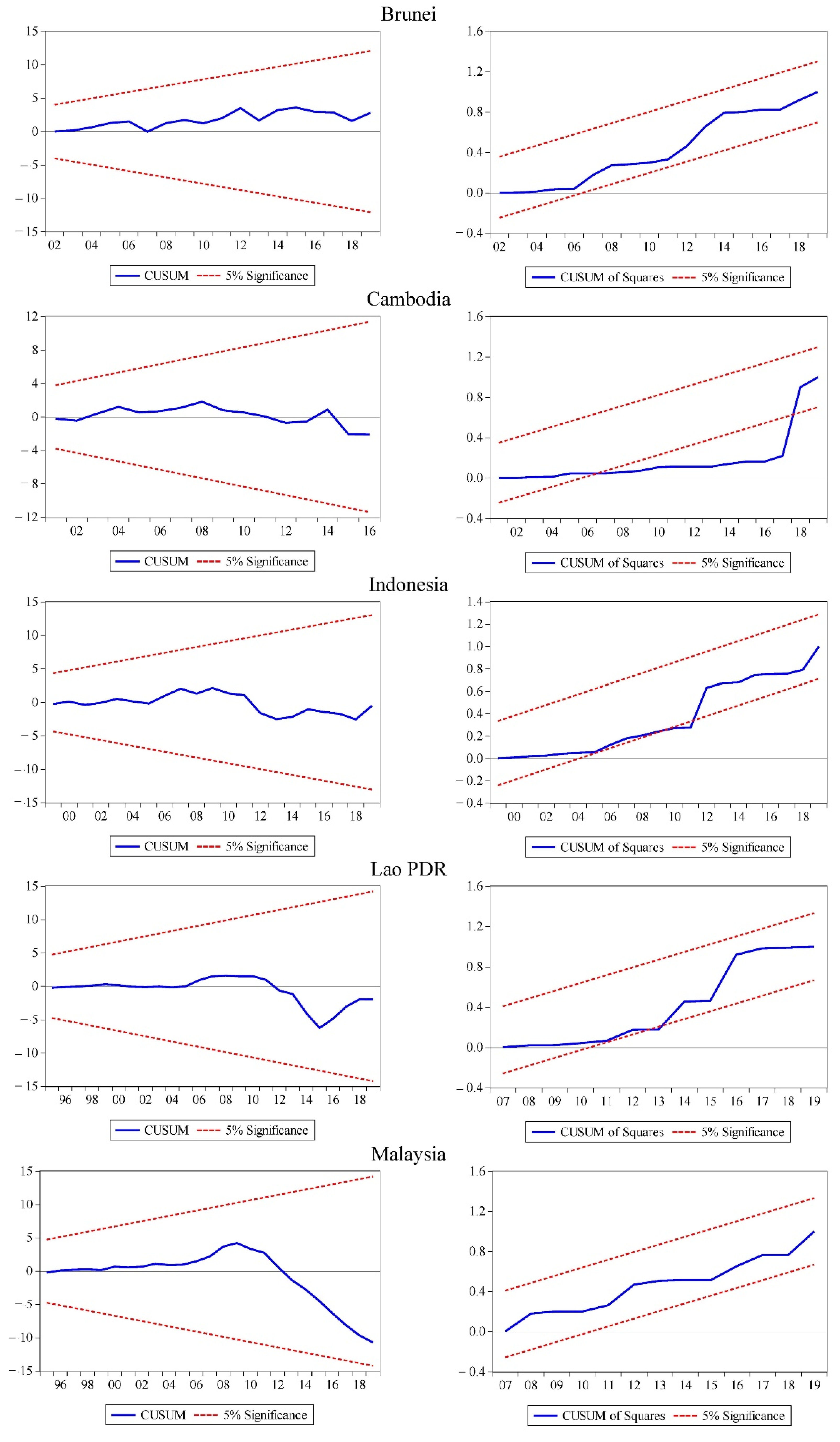
4.7. Findings of Stability Diagnostics

The study uses the CUSUM and CUSUMSQ tests to estimate and detect the structural break and the coefficient constancy and stability in the mode, respectively. The CUSUM and CUSUMSQ graphs are given in Figure 6 and Figure 7. In the figures, the two red lines indicate the critical bounds at a 5 percent significance level, while the blue line shows the process mean. In the CUSUM test, any value that lies outside the order indicates the structural change in the model over time. Likewise, in the CUSUMSQ test, any value that lies outside the sequence indicates the instability in the parameter coefficients within the model. It is observed that there are no change points/structural breaks in cross-sections. On the other hand, CUSUMSQ in Cambodia, Indonesia, Vietnam, and Singapore indicates the instability of parameters. Cambodia is the most volatile among the panel from 2006 to 2017. Indonesia, Vietnam, and Singapore face instability in parameters for a short period of time.

5. Discussion

In lower-middle-income economies (LMIE), the fiscal deficit (FD) has no long-run or short-run relationship with CAD. In fact, FD does not significantly induce CAD. Further, EXC and RIR can have a long-term influence on CAD. EXC is inversely associated with CAD, as depreciation in the exchange rate encourages exports, and with high exports, the current account deficit may decrease. When the interest rate increases, it encourages capital inflow and appreciation in the exchange rate, which may result in a deficit in current accounts. In LMIE, according to the results of the DH causality test, there is a unidirectional causal relationship from CAD to FD. This leads to reverse causality from the current account deficit to the fiscal deficit. This is known as the current account targeting hypothesis. Therefore, LMIE need to adjust the trade balance by utilizing fiscal policy tools. The transmission mechanism is that, when imports increase in LMIE, it induces an increase in government expenditures which leads to the fiscal deficit.
In UMIE, the real interest rate (RIR) has a positive long-run relationship with the current account deficit. The high-interest rate can increase imports and generates a current account deficit (imports > exports). This relationship is not sensitive, as the RIR coefficient value is less than unity (0.008) and approaches zero. EXC and FD are significant to CAD in the long run, and the two-year past lag of EXC and FD is significant in the short run and has an impact on GDP growth. Moreover, in UMIE, there is no causality found between FD and CAD, in line with the work of [49]. This type of causality supports Ricardian equivalence theory. These results support the independent causality hypothesis between FD and CAD. Further fiscal deficit positively causes interest rate, and interest rate causes exchange rate. These results disclose that an increase in fiscal deficit puts upward pressure on the interest rate, which leads to an influence on the exchange rate level.
In the HIE of ASEAN, interest rate and fiscal deficit influence CAD for the long-run term period. RIR has a significant relationship with CAD, revealing that capital inflows are encouraged when the interest rate is high. A fiscal deficit can induce current account balance via different transmission mechanisms. Therefore, the well-known mechanism is that an increase in government expenditures (fiscal deficit) puts upward pressures on the interest rate and capital inflow increases, encourages imports, and falls in net exports, which generates the deficit in current accounts. This channel is supported by the Mundell–Fleming model. The one-year period lag of fiscal deficit has a significant and inverse relationship with CAD. In other words, the past year of fiscal deficit does not encourage the imports, which improves the current account deficit.
This study disclosed different results in these groups of ASEAN. Table 18 illustrates the comparative analysis between ASEAN-10 and its three income groups.
In the HIE of ASEAN, there is a unidirectional causal relationship from CAD to FD, leading to reverse causality from the current account deficit to the fiscal deficit. This is known as the current account targeting hypothesis (CATH). Baharumshah et al. [19] mentioned that a high interest rate encourages foreign capital inflows, leads to an appreciated exchange rate, results in high government expenditures, and finally widens the fiscal deficit. The HIE (Singapore and Brunie) governments can exterminate the deficit in current accounts by utilizing the fiscal policy as a tool.

6. Conclusions

The primary aim of this study is to explore the causal relationship between fiscal and current account deficits in ASEAN income subgroups (LMIE, UMIE, and HIE). The study aims to, secondly, investigate the impact of fiscal deficit on current account deficit in the short run and long run and, thirdly, to explore the behavior of exchange and interest rate. Therefore, for the first objective, the study concludes that there is a current account targeting hypothesis supported in lower-middle-income economies (LMIE), which means reverse causality is found between fiscal and current account deficits in LMIE. It implies that current account imbalance is transmitted to national accounts, through the actions of automatic stabilizers, in an adverse way. In this case, the government has the main objective of reducing the unfavorable current account balance by utilizing the restrictive fiscal policy, which means reducing government expenditures and transferring and increasing revenues, among other tasks. Further, for the second and third objectives for LMIE, RIR and EXC have a significant long-run relationship with CAD, while no short relationship is found between the tested variables. RIR and EXC are influential to CAD in the long run and can be utilized for long-term policy implications.
In upper-middle-income economies (UMIE), there is no causality relationship found between fiscal and current account deficits. The Ricardian equivalence hypothesis is supported in UMIE. It states that an increase in tax rate can contract the fiscal deficit but may not change the trade balance. An increase in the fiscal deficit will not alter the capital inflows or the level of aggregate demand. Hence, in UMIE, fiscal deficit has no consequence on current account deficit. This is where government expenditures are not leading to an increase in imports and generating negative net exports. Further, EXC and FD have a long-run cointegrated relationship with CAD.
Interestingly, FD has a significant long-run relationship with CAD, but FD and CAD have no causality association. This case is unique because causality is different from single equation significance. Hence, in the long term, FD can have the consequence of CAD. In short-run dynamics, the two-year lags of EXC and FD have a significant influence on CAD. In higher-income economies (HIE), and likewise in LMIE, the current account targeting hypothesis is confirmed. FD and EXC are observed as influential on CAD in the long run, while in the short run RIR and the two-year past lag of FD has an impact on CAD. Moreover, the exchange rate plays an essential role as a moderator between FD and CAD in all three income sub-groups.

7. Policy Implications

After concluding the results, this study recommends a few policy implications, given below.
  • In LMIE, policy practitioners can target the current account balance, as it monitors the trade competitiveness to evaluate the flow of net exports. A unidirectional relationship from CAD to FD indicates that the current account is initiating the fiscal deficit, and external imbalance is transmitted to national accounts via automatic stabilizers.
  • The results for UMIE can illuminate to the policymakers that the fiscal deficit does not cause the trade balance in the context of the twin deficit hypothesis. However, the fiscal deficit can influence and has a consequence on the current account deficit in the long run. Hence, the fiscal deficit and the exchange rate can be the targeted factors for authorities.
  • Fiscal policy tools can be utilized to achieve favorable current accounts in HIE. Practitioners can target the current account balance to minimize the fiscal deficit. The current account targeting hypothesis (CATH) leads to monitoring the trade balance.

Author Contributions

Conceptualization and methodology, H.K. and M.M.; formal analysis, H.K., M.M. and R.B.; investigation, H.K. and M.M.; validation, H.K., M.M. and R.B.; writing—original draft preparation, H.K.; writing—review and editing, M.M. and R.B.; supervision, M.M. All authors have read and agreed to the published version of the manuscript.

Funding

This research was funded by the Universiti Teknologi PETRONAS, Malaysia, under the YUTP research project (no. 015LC0-194).

Institutional Review Board Statement

Not applicable.

Informed Consent Statement

Not applicable.

Data Availability Statement

Publicly available datasets from the World Bank’s Development Indicators and the Asian Development Bank Database were analyzed in this study. These data can be found here: World Bank: https://data.worldbank.org/ (accessed on 5 April 2022); ADB: https://data.adb.org/ (accessed on 6 April 2022).

Acknowledgments

This study is supported by Universiti Teknologi PETRONAS, Malaysia, and the Institute of Management Sciences (IM|Sciences), Pakistan.

Conflicts of Interest

The authors declare no conflict of interest. The funder had no role in the design of the study; in the collection, analyses, or interpretation of data; in the writing of the manuscript; or in the decision to publish the results.

References

  1. Marimuthu, M.; Khan, H.; Bangash, R. Fiscal causal hypotheses and panel cointegration analysis for sustainable economic growth in ASEAN. J. Asian Financ. Econ. Bus. 2021, 8, 99–109. [Google Scholar]
  2. Salvatore, D. Twin Deficits in the G-7 Countries and Global Structural Imbalances. J. Policy Model. 2006, 28, 701–712. [Google Scholar] [CrossRef]
  3. Lau, W.-Y.; Yip, T.-M. The Nexus between Fiscal Deficits and Economic Growth in ASEAN. J. Southeast Asian Econ. 2019, 36, 25–36. [Google Scholar] [CrossRef]
  4. Khan, H.; Marimuthu, M.; Lai, F.-W. A Granger Causal Analysis of Tax-Spend Hypothesis: Evidence from Malaysia. In Proceedings of the SHS Web of Conferences, Virtual, Malaysia, 13–15 July 2021; p. 04002. [Google Scholar]
  5. Ridzuan, M.R.; Abd Rahman, N.A.S. The Deployment of Fiscal Policy In Five ASEAN Countries in Dampening The Impact of COVID-19. J. Emerg. Econ. Islam. Res. 2021, 9, 16–28. [Google Scholar]
  6. Wijaya, S. Determinant of Value Added Tax Revenue in ASEAN (the Association of Southeast Asian Nations) Countries. Int. J. Manag. 2020, 11, 1453–1463. [Google Scholar]
  7. Widiyanti, M.; Sadalia, I.; Nugraha, A.T. Integrating Fiscal Matters with Environmental Sustainability In ASEAN Countries: Role Of Fiscal Deficit, Interest Rate And Stock Exchange Index. J. Secur. Sustain. Issues 2020, 10, 349–359. [Google Scholar] [CrossRef]
  8. Ngo, M.N.; Nguyen, L.D. The Role of Economics, Politics and Institutions on Budget Deficit in ASEAN Countries. J. Asian Financ. Econ. Bus. 2020, 7, 251–261. [Google Scholar] [CrossRef]
  9. Fitriaini, R. Fiscal Policy Behaviour in ASEAN: Countercyclical or Procyclical? KnE Soc. Sci. 2020, 4, 170–178. [Google Scholar] [CrossRef]
  10. Alwan, F.; Hakim, L.; Saputro, N. The Pattern of Twin Deficits in ASEAN: Granger Casuality Approach. Issues Incl. Growth Dev. Ctries. 2020, 1, 01–12. [Google Scholar]
  11. Chen, L. ASEAN in the Digital Era: Enabling Cross-border E-commerce. In Developing the Digital Economy in ASEAN; Chen, L., Kimura, F., Eds.; Routledge: London, UK, 2019; pp. 259–275. [Google Scholar]
  12. Abdullah, H.; Yien, L.C.; Khan, M.A. The impact of fiscal policy on economic growth in ASEAN-5 countries. Int. J. Supply Chain. Manag. 2019, 8, 754. [Google Scholar]
  13. Thanh, S.D. Threshold effects of inflation on growth in the ASEAN-5 countries: A Panel Smooth Transition Regression approach. J. Econ. Financ. Adm. Sci. 2015, 20, 41–48. [Google Scholar] [CrossRef]
  14. Syadullah, M. Governance and tax revenue in ASEAN countries. J. Soc. Dev. Sci. 2015, 6, 76–88. [Google Scholar] [CrossRef]
  15. Magazzino, C. The twin deficits in the ASEAN countries. Evol. Inst. Econ. Rev. 2021, 18, 227–248. [Google Scholar] [CrossRef]
  16. Chugunov, I.; Makohon, V.; Krykun, T. Fiscal policy and institutional budget architectonics. Balt. J. Econ. Stud. 2019, 5, 197–203. [Google Scholar] [CrossRef]
  17. Shastri, S. Re-examining the Twin Deficit Hypothesis for Major South Asian Economies. Indian Growth Dev. Rev. 2019, 12, 265–287. [Google Scholar] [CrossRef]
  18. Shastri, S.; Giri, A.; Mohapatra, G. An empirical Investigation of the Twin Deficit Hypothesis: Panel Evidence from Selected Asian Economies. J. Econ. Res. 2017, 22, 1–22. [Google Scholar]
  19. Baharumshah, A.Z.; Ismail, H.; Lau, E. Twin Deficits Hypothesis and Capital Mobility: The ASEAN-5 Perspective. J. Pengur. 2009, 29, 15–32. [Google Scholar]
  20. Keynes, J.M. The general theory of employment. Q. J. Econ. 1937, 51, 209–223. [Google Scholar] [CrossRef]
  21. Mundell, R.A. Capital mobility and stabilization policy under fixed and flexible exchange rates. Can. J. Econ. Political Sci./Rev. Can. Econ. Sci. Polit. 1963, 29, 475–485. [Google Scholar] [CrossRef]
  22. Fleming, J.M. Domestic financial policies under fixed and under floating exchange rates. Staff Pap. 1962, 9, 369–380. [Google Scholar] [CrossRef]
  23. Buchanan, J.M. Barro on the Ricardian equivalence theorem. J. Political Econ. 1976, 84, 337–342. [Google Scholar] [CrossRef]
  24. Summers, L.H. Tax Policy and International Competitiveness. In International Aspects of Fiscal Policies; University of Chicago Press: Chicago, IL, USA, 1988; pp. 349–386. [Google Scholar]
  25. Kim, C.-H.; Kim, D. Does Korea have Twin Deficits? Appl. Econ. Lett. 2006, 13, 675–680. [Google Scholar] [CrossRef]
  26. Lau, E.; Mansor, S.A.; Puah, C.-H. Revival of the Twin Deficits in Asian Crisis-Affected Countries. Econ. Issues 2010, 15, 29–53. [Google Scholar]
  27. Maddala, G.S.; Wu, S. A Comparative Study of Unit Root Tests with Panel Data and a New Simple Test. Oxf. Bull. Econ. Stat. 1999, 61, 631–652. [Google Scholar] [CrossRef]
  28. Westerlund, J. Testing for panel cointegration with multiple structural breaks. Oxf. Bull. Econ. Stat. 2006, 68, 101–132. [Google Scholar] [CrossRef]
  29. Marimuthu, M.; Khan, H.; Bangash, R. Is the Fiscal Deficit of ASEAN Alarming? Evidence from Fiscal Deficit Consequences and Contribution towards Sustainable Economic Growth. Sustainability 2021, 13, 10045. [Google Scholar] [CrossRef]
  30. Marimuthu, M.; Khan, H.; Bangash, R. Reverse Causality between Fiscal and Current Account Deficits in ASEAN: Evidence from Panel Econometric Analysis. Mathematics 2021, 9, 1124. [Google Scholar] [CrossRef]
  31. Dumitrescu, E.-I.; Hurlin, C. Testing for Granger Non-causality in Heterogeneous Panels. Econ. Model. 2012, 29, 1450–1460. [Google Scholar] [CrossRef] [Green Version]
  32. Shah, M.I. Current account deficit across South Asia: A Second Generation Methodological Adaptive Approach. J. Public Aff. 2020, 22, e2475. [Google Scholar] [CrossRef]
  33. Garg, B.; Prabheesh, K. Drivers of India’s current account deficits, with implications for ameliorating them. J. Asian Econ. 2017, 51, 23–32. [Google Scholar] [CrossRef]
  34. Khan, H.; Marimuthu, M.; Lai, F.-W. Fiscal Deficit and Its Less Inflationary Sources of Borrowing with the Moderating Role of Political Instability: Evidence from Malaysia. Sustainability 2020, 12, 366. [Google Scholar] [CrossRef]
  35. Levin, A.; Lin, C.-F.; Chu, C.-S.J. Unit root tests in panel data: Asymptotic and finite-sample properties. J. Econom. 2002, 108, 1–24. [Google Scholar] [CrossRef]
  36. Im, K.S.; Pesaran, M.H.; Shin, Y. Testing for unit roots in heterogeneous panels. J. Econom. 2003, 115, 53–74. [Google Scholar] [CrossRef]
  37. Baltagi, B.H. Econometric Analysis of Panel Data, 6th ed.; Springer Nature: Cham, Switzerland, 2021. [Google Scholar]
  38. Hall, S.G.; Asteriou, D. Applied Econometrics; Palgrave MacMillan: London, UK, 2016. [Google Scholar]
  39. Asteriou, D.; Hall, S.G. Applied Econometrics, 3rd ed.; Macmillan International Higher Education: Basingstoke, UK, 2015. [Google Scholar]
  40. Kao, C.; Chiang, M.-H. On the estimation and inference of a cointegrated regression in panel data. In Nonstationary Panels, Panel Cointegration, and Dynamic Panels; Baltagi, B.H., Fomby, T.B., Carter Hill, R., Eds.; Advances in Econometrics; Emerald Group Publishing Limited: Bentley, UK, 2001; Volume 15, pp. 179–222. [Google Scholar]
  41. Rahman, M.M.; Hosan, S.; Karmaker, S.C.; Chapman, A.J.; Saha, B.B. The effect of remittance on energy consumption: Panel cointegration and dynamic causality analysis for South Asian countries. Energy 2021, 220, 119684. [Google Scholar] [CrossRef]
  42. Arize, A.C.; Osang, T.; Slottje, D.J. Exchange-rate volatility and foreign trade: Evidence from thirteen LDC’s. J. Bus. Econ. Stat. 2000, 18, 10–17. [Google Scholar]
  43. Arize, A.C.; Malindretos, J.; Ghosh, D. Purchasing power parity-symmetry and proportionality: Evidence from 116 countries. Int. Rev. Econ. Financ. 2015, 37, 69–85. [Google Scholar] [CrossRef]
  44. Baltagi, B.H. Econometric Analysis of Panel Data, 3rd ed.; Wiley: New York, NY, USA, 2005. [Google Scholar]
  45. Antoch, J.; Hanousek, J.; Horváth, L.; Hušková, M.; Wang, S. Structural breaks in Panel Data: Large Number of Panels and Short Length Time Series. Econom. Rev. 2019, 38, 828–855. [Google Scholar] [CrossRef]
  46. Maciak, M.; Pešta, M.; Peštová, B. Changepoint in Dependent and Non-stationary Panels. Stat. Pap. 2020, 61, 1385–1407. [Google Scholar] [CrossRef]
  47. Pedroni, P. Panel cointegration: Asymptotic and finite sample properties of pooled time series tests with an application to the PPP hypothesis. Econom. Theory 2004, 20, 597–625. [Google Scholar] [CrossRef] [Green Version]
  48. Marques, A.C.; Fuinhas, J.A.; Pais, D.F. Economic growth, sustainable development and food consumption: Evidence across different income groups of countries. J. Clean. Prod. 2018, 196, 245–258. [Google Scholar] [CrossRef]
  49. Badaik, S.; Panda, P.K. Ricardian equivalence, Feldstein–Horioka puzzle and twin deficit hypothesis in Indian context: An empirical study. J. Public Aff. 2020, 22, e2346. [Google Scholar] [CrossRef]
Figure 1. ASEAN’s income sub-groups on the basis of GNI per capita. Source: ESCAP (based on World Economic Outlook databases).
Mathematics 10 03259 g001
Figure 2. Fiscal and Current Account Deficits in ASEAN.
Mathematics 10 03259 g002
Figure 3. Mundell–Fleming model and expansionary fiscal policy. Y refers to Y-axis, and Y 1 , Y 2 refer to output. The * represents the initial values.
Mathematics 10 03259 g003
Figure 4. ASEAN-5 current account balance and investment, % of GDP (1980–2018). Source: IMF World Economic Outlook (WEO). ASEAN-5 includes Malaysia, Indonesia, Philippines, Singapore, and Thailand.
Mathematics 10 03259 g004
Figure 5. Expansionary fiscal policy and exchange rate.
Mathematics 10 03259 g005
Figure 6. Findings of stability test (structural breaks and coefficient stability test).
Mathematics 10 03259 g006
Figure 7. Findings of stability test (structural breaks and coefficient stability test).
Mathematics 10 03259 g007
Table 1. The fiscal position of Malaysia (member of UMIE) during the first five months of 2019 and 2018 (MYR billions).
ItemJanuary–May (2019)January–May (2018)Difference
Revenues105.492.712.7
Operating expenditures106.5109.9−3.3
Current account balance−1.1−17.116.0
Development expenditures20.317.92.4
Fiscal balance−21.4−35.013.6
Source: Ministry of Finance, Malaysia (https://budget.mof.gov.my/en/fiscal/) accessed on 9 August 2022.
Table 2. ASEAN expenditures to support COVID-19.
S. No.ASEAN-10Fiscal Deficit (% of GDP)Expenditures to Support COVID-19 (% of GDP)
1.Brunei Darussalam−17.947.4
2.Cambodia−6.52.3
3.Indonesia−6.612.3
4.Lao PDR−7.502.9
5.Malaysia−6.5320.29
6.Myanmar−5.419
7.Philippines−7.55.83
8.Singapore−10.7719.88
9.Thailand−5.2111.5
10.Vietnam−6.0214.6
Table 3. Theoretical Background.
Author (Year)Description
Keynesian absorption theory [20]An increase in fiscal budget leads to an increase in aggregate demand, which puts upward pressure on imports and causes an increase in CAD.
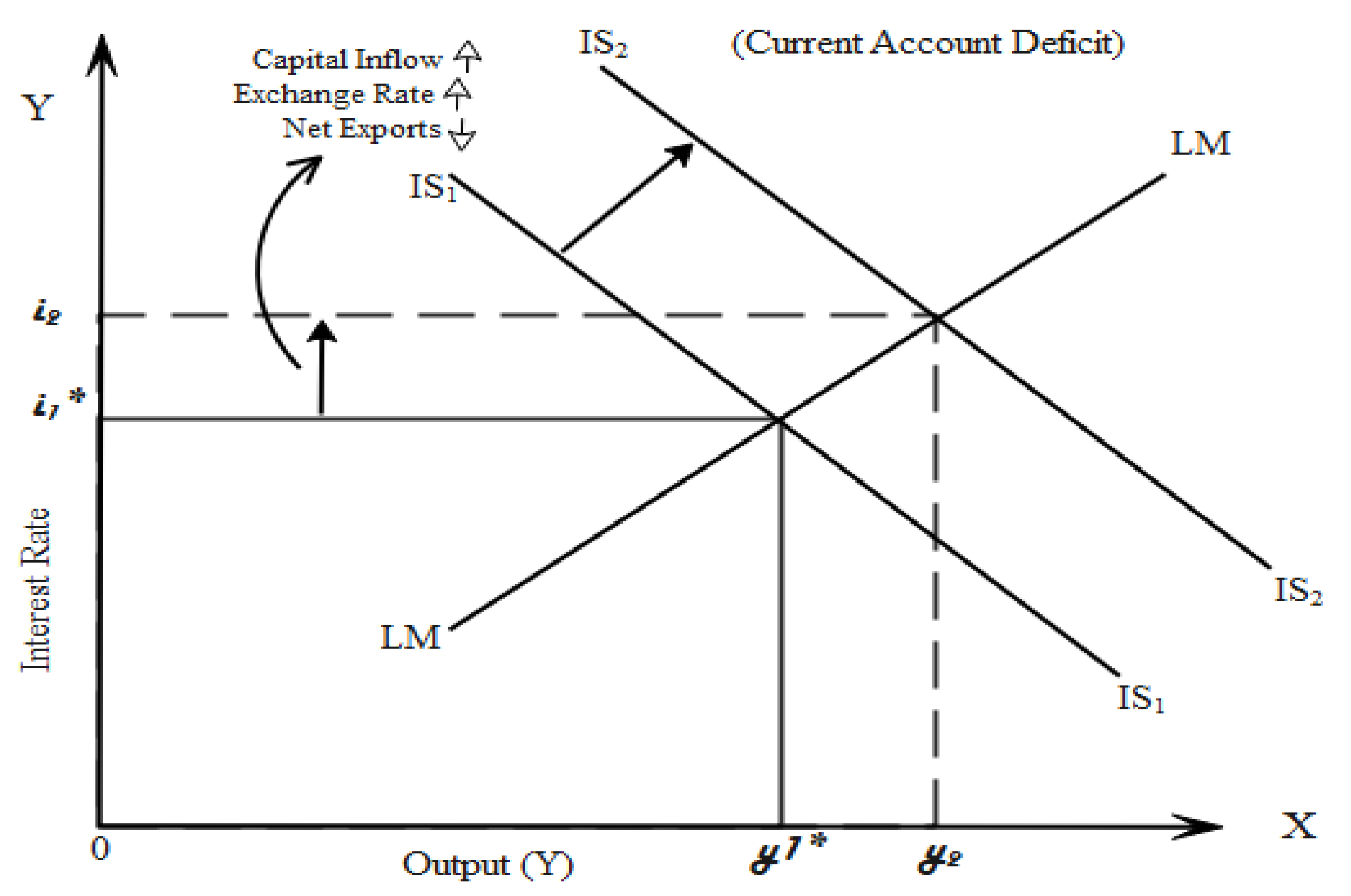
Mundell and Fleming’s theory (1960s) [21,22]An increase in fiscal deficit puts upward pressure on the interest rate, increasing capital inflow and appreciation in the exchange rate. This channel ultimately exacerbates the trade balance. Therefore, the first possibility indicates that causality runs from FD to CAD.
Ricardian equivalence (RE) theory [23]An increase in tax rate can contract the fiscal deficit but may not change the trade balance. The RE theory suggests that an increase in the fiscal deficit will not alter the capital inflows and level of aggregate demand. The second possibility refers to no causality between CAD and FD.
Neo-classical theory [24]The fiscal deficit can be used as an instrument to achieve the current account balance. The government uses its fiscal policy to regulate the external balance. This case refers to reverse causality, in which causality runs from current account deficit to fiscal deficit. This is known as the current account targeting hypothesis (CATH), where unidirectional causality runs from CAD to FD.
Kim and Kim [25]Causality from CAD to FD refers to external adjustments through fiscal policy, while causality from FD to CAD may result from significant feedback. Therefore, in this way, bidirectional causality may occur between FD and CAD.
Table 4. Variables, Data Sources, and Units.
Gross Domestic ProductWorld Bank Data Bank 2020Million Dollars
Fiscal deficitAsian Development Bank 2020In percentages
Current account deficitAsian Development Bank 2020Million dollars
Official exchange rateWorld Bank, Databank 2020Rate variable
Real interest rateWorld Bank, Databank 2020Rate variable
Table 5. Findings of panel unit root testing for lower-middle-income economies (LMIE).
Im, Pesaran, and Shin (Individual Root)Levin, Lin, and Chu (Common Unit Root Process)
VariableAt LevelAt First DifferenceAt LevelAt First Difference
Gross domestic product (GDP)1.26 (0.897)−3.56 (0.000) ***(At none)3.14 (0.99)−5.83 (0.001) ***(At individual intercept)
Fiscal deficit (FD)−0.89 (0.185)−4.33 (0.001) ***(At individual intercept)0.05 (0.52)−4.64 (0.000) ***(At individual intercept and trend)
Real interest rate (RIR)−2.40 (0.008)-(At none)−3.29 (0.00)-(At individual intercept and trend)
Current account deficit (CAD)3.68 (0.999)−2.99 (0.001) ***(At individual intercept)2.89 (0.99)−5.69 (0.002) ***(At individual intercept)
Exchange rate (EXC)1.58 (0.943)−6.19 (0.001) ***(At none)−0.72 (0.23)−3.98 (0.000) ***(At individual intercept)
Note: *** represents significance at 1%; value in brackets presents p-values. Without brackets indicate t-statistic values.
Table 6. Findings of panel unit root testing for upper-middle-income economies (UMIE).
Im, Pesaran, and Shin (Individual Root)Levin, Lin, and Chu (Common Unit Root Process)
VariablesAt LevelAt First DifferenceAt LevelAt First Difference
Gross domestic product (GDP)0.20 (0.580)−2.88 (0.001) ***(At individual intercept)1.93 (0.970)−3.69 (0.000) ***(At individual intercept)
Fiscal deficit (FD)−0.25 (0.400)−4.79 (0.001) ***(At individual intercept)−1.14 (0.120)−6.58 (0.001) ***(At individual intercept)
Real interest rate (RIR)−2.81 (0.002) ***-(At individual intercept)−2.50 (0.006) ***-(At individual intercept)
Current account deficit (CAD)−3.52 (0.000) ***-(At individual intercept)−3.99 (0.001) ***-(At individual intercept)
Exchange rate (EXC)−0.41 (0.340)−6.25 (0.002) ***(At individual intercept and trend)−0.05 (0.472)−4.46 (0.001) ***(At individual intercept)
Note: *** represents significance at 1%; value in brackets presents p-values. Without brackets indicate t-statistic values.
Table 7. Findings of panel unit root testing for higher-income economies (HMIE).
Im, Pesaran, and Shin (Individual Root)Levin, Lin, and Chu (Common Unit Root Process)
VariableAt LevelAt First DifferenceAt LevelAt First Difference
Gross domestic product (GDP)0.40 (0.65)−1.76 (0.03) **(At individual intercept)1.28 (0.90)−2.16 (0.01) **(At individual intercept)
Fiscal deficit (FD)0.52 (0.29)−3.81 (0.00)(At individual intercept)0.98 (0.16)5.07 (0.00) ***(At individual intercept)
Real interest rate (RIR)−2.79 (0.00) ***-(At individual intercept)−2.41 (0.00) ***-(At individual intercept)
Current account deficit (CAD)0.57 (0.71)−6.12 (0.00) ***(At none)−0.07 (0.47)−4.20 (0.00)(At individual intercept)
Exchange rate (EXC)−0.46 (0.32)−2.83 (0.00) ***(At individual intercept and trend)−0.40 (0.34)−2.19 (0.01) **(At individual intercept)
Note: ***, ** represents significance at 1%, and 5%, respectively; value in brackets presents p-values. Without brackets indicate t-statistic values.
Table 8. Fixed and Random Effects for Panel Data.
Lower-Middle-Income EconomiesChow TestLagrange Multiplier TestHausman Test
H0: Common Effect
H1: Fixed Effects
H0: Common Effects
H1: Random Effects
H0: Random Effects
H1: Fixed Effects
Decision: select CE (accept H0)Decision: select RE (reject H0)Decision: random effects (accept H0)
Cross-section dependence testPesaran CD: 0.58
Prob. = 0.41
N < T (cross-sections are independent)
Upper-middle-income economiesH0: common effect
H1: fixed effects
H0: common effects
H1: random effects
H0: random effects
H1: fixed effects
Decision: select CE (accept H0)Decision: select RE (reject H0)Decision: random effects (accept H0)
Cross-section dependence testPesaran CD: 0.75
Prob. = 0.29
N < T (cross-sections are independent)
Higher-income economiesH0: common effect
H1: fixed effects
H0: common effects
H1: random effects
H0: random effects
H1: fixed effects
Decision: select CE (accept H0)Decision: select RE (reject H0)Decision: random effects (accept H0)
Cross-section dependence testPesaran CD: 0.44
Prob. = 0.41
N < T (cross-sections are independent)
Table 9. Results of panel EGLS (random effects).
Dependent Variable
CAD
Coefficientt-Statisticp-Value
Lower-middle-income economies
Exchange rate (EXC)−0.28−1.270.21
Real interest rate (RIR)0.068.570.00 ***
Fiscal deficit (FD)0.0080.810.40
Upper-middle-income economies
Exchange rate (EXC)−0.53−2.050.04 **
Real interest rate (RIR)0.022.0770.03 **
Fiscal deficit (FD)0.041.540.13
Higher-income economies
Exchange rate (EXC)0.081.490.13
Real interest rate (RIR)0.122.620.01 **
Fiscal deficit (FD)0.011.330.19
Note: ***, ** represents significance at 1%, and 5%, respectively.
Table 10. Findings of panel auto-regressive distributed lag (ARDL) for lower-middle-income economies (LMIE).
Dependent Variable
CAD
CoefficientStd. Errort-Statisticp-Value
Long-run equation
Exchange rate (EXC)−0.140.22−1.850.04 **
Real interest rate (RIR)0.040.0094.950.00 ***
Fiscal deficit (FD)0.0030.0080.460.64
Short-run equation
COINTEQ01−0.780.14−5.210.00 ***
Δ (CAD(−1))0.040.050.810.42
Δ (EXC)1.412.130.660.50
Δ (EXC(−1))0.801.180.670.50
Δ (RIR)0.010.030.390.69
Δ (RIR(−1))−0.0140.01−1.230.22
Δ (FD)−0.010.06−0.230.81
Δ (FD(−1))−0.020.02−0.750.45
Gross domestic product (GDP)0.930.224.114.11
Constant (C)−1.791.48−1.210.22
Note: The model selection is AIC (Akaike information criterion), dependent lags are two (automatic selection), GDP is utilized as a fixed regressor, and the model selection is ARDL (2,2,2,2), with ***, ** representing significance at 1% and 5%, respectively. Value in brackets presenting p-values. This table note applies to Table 11 and Table 12 as well.
Table 11. Findings of panel auto-regressive distributed lag (ARDL) for upper-middle-income economies (UMIE).
Dependent Variable
CAD
CoefficientStd. Errort-Statisticp-Value
Long-run equation
Exchange rate (EXC)0.190.350.540.58
Real interest rate (RIR)0.040.022.130.03 **
Fiscal deficit (FD)0.080.071.010.32
Short-run equation
COINTEQ01−0.690.32−2.110.03 **
Δ (EXC)1.180.811.450.15
Δ (EXC(−1))1.630.552.940.004 ***
Δ (RIR)−0.010.01−1.640.10
Δ (RIR(−1))−0.010.02−0.690.49
Δ (FD)0.060.061.060.28
Δ (FD(−1))0.050.021.980.05 **
Gross domestic product (GDP)0.710.451.580.11
Constant (C)−2.043.23−0.630.52
Note: ***, ** represents significance at 1%, and 5%, respectively.
Table 12. Findings of panel auto-regressive distributed lag (ARDL) for higher-income economies (HMIE).
Dependent Variable
CAD
CoefficientStd. Errort-Statisticp-Value
Long-run equation
Exchange rate (EXC)0.460.560.820.41
Real interest rate (RIR)0.0060.0032.240.03 **
Fiscal deficit (FD)0.020.00114.40.00 ***
Short-run equation
COINTEQ01−0.980.08−11.770.00 ***
Δ (EXC)3.031.811.670.10
Δ (EXC(−1))−3.622.24−1.610.11
Δ (RIR)−0.020.01−1.910.06 *
Δ (RIR(−1))−0.00080.006−0.110.90
Δ (FD)0.0020.020.090.92
Δ (FD(-1))−0.010.001−6.910.00 ***
Gross domestic product (GDP)0.380.301.260.21
Constant (C)4.874.231.150.25
Note: ***, **, * represents significance at 1%, 5% and 10%, respectively.
Table 13. Findings of FMOLS and DOLS for LMIE.
VariablesFMOLSDOLS
Dependent Variable CADCoefficientt-Statistics
(p-Value)
Coefficientt-Statistics
(p-Value)
RIR0.052.33 (0.030) **0.031.91 (0.041) **
EXC0.071.93 (0.040) **0.281.60 (0.110)
FD−0.02−1.30 (0.191)0.0050.892
GDP0.987.94 (0.000) ***1.355.88 (0.000) ***
R20.70 0.88
Note: the values with ***, **, represent significance at levels 1%, and 5%, respectively.
Table 14. Findings of FMOLS and DOLS for UMIE.
VariablesFMOLSDOLS
Dependent Variable CADCoefficientt-Statistics
(p-Value)
Coefficientt-Statistics
(p-Value)
RIR0.0080.81 (0.411)0.0080.76 (0.440)
EXC−0.12−2.47 (0.010) **−0.09−1.85 (0.060) *
FD0.071.95 (0.050) **0.071.91 (0.050) **
GDP0.8753.61 (0.000) ***0.8649.76 (0.000) ***
R20.72 0.82
Note: the values with ***, **, and * represent significance at levels 10%, 5% and 1%, respectively.
Table 15. Findings of FMOLS and DOLS for HIE.
VariablesFMOLS DOLS
Dependent Variable CADCoefficientt-Statistics
(p-Value)
Coefficientt-Statistics
(p-Value)
RIR−0.001−0.35 (0.720)−0.01−0.94 (0.350)
EXC−3.53−3.06 (0.003) **−4.67−2.63 (0.010) **
FD0.013.80 (0.000) ***0.022.74 (0.010) **
GDP0.8015.36 (0.000) ***0.7213.21(0.020) **
R20.40 0.78
Note: the values with *** and ** represent significance at levels 1% and 5%, respectively.
Table 16. Findings of DH Granger causality for three income groups.
Null HypothesisW-StatZbar-Statp-Value
Lower-middle-income economies (LMIE)
CA↛FD
FD↛CAD
4.68
1.81
2.28
−0.35
0.021 **
0.722
RIR↛CAD
CAD↛RIR
2.38
1.08
0.41
−1.02
0.680
0.300
FD↛EXC
EXC↛FD
0.90
0.63
−1.18
−1.43
0.230
0.150
FD↛IR
RIR↛FD
0.28
1.20
−1.76
−0.91
0.070 *
0.362
EXC↛RIR
RIR↛EXC
6.10
3.79
3.58
1.46
0.000 ***
0.141
EXC↛CAD
CAD↛EXC
2.38
0.71
0.17
−1.36
0.862
0.173
Upper-middle-income economies (UMIE)
CA↛FD
FD↛CAD
0.33
0.78
−1.32
−1.007
0.182
0.311
RIR↛CAD
CAD↛RIR
2.59
0.24
0.28
−1.39
0.777
0.166
FD↛EXC
EXC↛FD
1.34
0.82
−0.60
−0.97
0.544
0.322
FD↛RIR
RIR↛FD
5.31
1.92
2.21
−0.19
0.020 **
0.840
EXC↛RIR
RIR↛EXC
3.00
5.97
0.57
2.68
0.560
0.007 ***
EXC↛CAD
CAD↛EXC
0.78
1.89
−1.00
−0.22
0.311
0.822
Higher-income economies (HIE)
CA↛FD
FD↛CAD
11.95
0.94
5.67
−0.73
0.000 ***
0.460
RIR↛CAD
CAD↛RIR
1.43
1.65
−0.44
−0.31
0.650
0.752
FD↛EXC
EXC↛FD
1.41
0.72
−0.45
−0.85
0.643
0.396
FD↛RIR
RIR↛FD
0.60
1.09
−0.93
−0.64
0.355
0.522
EXC↛RIR
RIR↛EXC
5.89
2.52
2.14
0.19
0.033 **
0.840
EXC↛CAD
CAD↛EXC
2.94
2.10
0.43
−0.05
0.666
0.955
Note: *, **, and *** represent significance at 10%, 5%, and 1%, respectively. The lag is 2. The symbol ‘↛’ refers to ‘does not cause’.
Table 17. Diagnostic checks for endogeneity and heterogeneity in the models.
Lower-Middle-Income Economies (LMIE)
ModelOmitted Variable TestSpecification TestHeteroscedasticity
TESTLikelihood ratioHausman testBreusch–Pagan
HypothesesHo: omitted variable is irrelevantHo: no omitted variableHo: constant variance
Equation (2)0.41 (p-value)0.31 (p-value)0.07 *
Upper-middle-income economies (UMIE)
Equation (2)0.22 (p-value)0.16 (p-value)0.09 *
Higher-income economies (HIE)
Equation (2)0.35 (p-value)0.19 (p-value)0.11
Table 18. Comparison between ASEAN-10, LMIE, UMIE, and HIE.
Lower-Middle-Income Economies (LMIE)Upper-Middle-Income Economies (UMIE)Higher-Income-Economies (HIE)
Current Account DeficitCATH (unidirectional causality)No causality
(CAD and FD are independent)
CATH (unidirectional causality)
RIRSignificantInsignificantInsignificant
EXCSignificantSignificantSignificant
FDInsignificantSignificantSignificant
RIR is less sensitive/elastic to CADEXC and FD are less sensitive/elastic to CADEXC is more sensitive/elastic to CAD
Publisher’s Note: MDPI stays neutral with regard to jurisdictional claims in published maps and institutional affiliations.

