Classification in High Dimension Using the Ledoit–Wolf Shrinkage Method

Abstract

Classification using linear discriminant analysis (LDA) is challenging when the number of variables is large relative to the number of observations. Algorithms such as LDA require the computation of the feature vector’s precision matrices. In a high-dimension setting, due to the singularity of the covariance matrix, it is not possible to estimate the maximum likelihood estimator of the precision matrix. In this paper, we employ the Stein-type shrinkage estimation of Ledoit and Wolf for high-dimensional data classification. The proposed approach’s efficiency is numerically compared to existing methods, including LDA, cross-validation, gLasso, and SVM. We use the misclassification error criterion for comparison.

1. Introduction

As one of the most widely used classification techniques, linear discriminant analysis (LDA) is still interesting because of its simplicity, stability, and prediction accuracy. Consider X as a p-dimensional predictor vector and the response $Y\in \{1,2,\dots ,K\}$ as the class labels. In LDA, it is assumed that $\mathit{X}|Y\sim N_p({\mathit{\mu }}_Y,\mathbf{\Sigma })$, where ${\mathit{\mu }}_Y\in {\mathbb{R}}^p$ and $\mathbf{\Sigma }>0$; consequently, the Bayes decision rule involves ${\mathbf{\Sigma }}^{-\mathbf{1}}$. In the large sample setting, when $p<n$, the sample covariance matrix $\mathbf{S}$ is an unbiased estimator of $\mathbf{\Sigma }$. However, in a high-dimensional setting, $p\approx n$ or $p>n$, $\mathbf{S}$ will be singular, and the likelihood estimator has many weaknesses such as inaccuracy (see [1,2]).

Many studies have been conducted using factor methods, sparse, graphical, and shrinkage methods for estimating $\mathbf{\Sigma }$. Srivastava [3] examined multivariate theory in a high-dimensional state and used the Moore–Penrose inverse of the covariance matrix to solve the singularity problem of $\mathbf{S}$. However, when some covariance matrix values are zero or close to zero, this idea does not work well.

The idea of estimating the precision matrix using a sparse method was first proposed by Dempster [4], and later, Meinshausen and Bühlmann [5] proposed the use of least absolute shrinkage and selection operator (Lasso) regression to identify the zeros of the inverse covariance matrix. Banerjee et al. [6] performed a penalized maximum likelihood estimation with the lasso penalty for sparse estimation of the inverse of the covariance matrix. Friedman et al. [7], proposed the graphical Lasso method, under the sparsity assumption of $\mathsf{\Theta }={\mathbf{\Sigma }}^{-\mathbf{1}}$ by using coordinate descent for the lasso penalty, through the objective function

$$logdet\mathsf{\Theta }-tr\mathbf{S}\mathsf{\Theta }-{\lambda \parallel \mathsf{\Theta }\parallel }_1,$$

(1)

where $\mathsf{\Theta }>0$, $tr\left(\mathit{A}\right)$ denotes the trace of matrix $\mathit{A}$, and ${\parallel .\parallel }_1$ is the norm one operator. Bickel and Levina [8] used the hard thresholding estimator for the sparse estimation of the covariance matrix $\mathbf{\Sigma }$. Furthermore, Cai and Zhang [9] developed an optimality theory for LDA in the high-dimensional setting by considering a different approach to solve the problem of LDA. Instead of estimating $\delta =({\mathit{\mu }}_{\mathbf{2}}-{\mathit{\mu }}_{\mathbf{1}})$, and $\mathsf{\Theta }={\mathbf{\Sigma }}^{-\mathbf{1}}$ separately, they proposed a data-driven and tunning free classification rule called AdaLDA by directly estimating the discriminant direction $\mathit{\beta }=\mathsf{\Theta }\delta$ through solving an optimization problem. As the hard threshold estimator in regression provides inflexible estimators, Ratman et al. [10] refined a generalized threshold law by using the combination of the threshold method and the shrinkage method. Bin and Tibshirani [11] generalized the estimate of a sparse covariance matrix by simultaneously estimating the nonzero covariance and the graph structure (location of zeros). Refer to Fan et al. [12] for more related studies.

Apart from sparse covariance matrix estimation, a common approach to improve the estimation of $\mathbf{\Sigma }$ is the use of the class of shrinkage estimators, which was initially proposed by James and Stein [13] to define bias estimation in order to reduce the variance of $\mathbf{S}$ (see [14,15,16] for extensive reviews). Di Pillo [17] and Campbell [18] improved the estimate of ${\mathbf{\Sigma }}^{-\mathbf{1}}$ using the ridge idea. Peck and Van Niss [2] proposed another type of shrinkage estimator of ${\mathbf{\Sigma }}^{-\mathbf{1}}$ by reducing the Fisher’s classification error. Mkhadri [19] used the cross-validation (CV) method to estimate the shrinkage parameter for the estimation of ${\mathbf{\Sigma }}^{-\mathbf{1}}$ in classification rule. However, Choi et al. [20] demonstrated that the use of the CV method may not lead to a positive definite estimate for the high-dimensional case $n\ll p$.

In the shrinkage method and graphical and factor models, additional information is needed in the estimation process (e.g., Beckel and Levina [21]; Khare and Rajaratnam [22]; Cai and Zhou [23]), whereas this surplus knowledge is not always available (Maurya [24]). Therefore, Ledoit and Wolf [25] proposed the rule of the optimal linear shrinkage estimator with optimal asymptotic properties by using the analysis of covariance matrix eigenvalues. For estimating the inverse covariance matrix (precision matrix) when $p\ge n$, other studies have been conducted such as Wang et al. [26], Hong and Kim [27], and Lee et al. [28].

This paper aims to classify high-dimensional observations using the LDA, where the inverse sample covariance matrix is singular and not invertible. We apply Lediot and Wolf’s shrinkage method to estimate $\mathsf{\Theta }$ and efficiently classify new observations in a high-dimensional regime. Thus, the plan for the rest of this paper is as follows. In Section 2, the proposed methodology, along with some theory, is given. Section 3 includes extensive numerical assessments for performance analysis and compares the proposed discriminant rule with other existing methods. We conclude with the significant results in Section 4; Appendix A is allocated for the proofs.

2. Materials and Methods

In discriminant analysis, a set of observations are classified into predetermined categories using a function called the decision function or discriminant function. In other words, discriminant analysis seeks to identify linear or nonlinear combinations of independent variables that are best able to separate groups of observations using the discriminant rule.

Consider distinct populations ${\Pi }_1,\dots ,{\Pi }_K$ with density function $f_j\left(x\right);j=1,2,\dots ,K$ and prior probabilities ${\pi }_j=Pr(Y\in {\Pi }_j)$. An observation $x$ is classified into ${\Pi }_i$ if

$$x\in {\Pi }_i⟺i=\underset{j}{arg\; max}{\pi }_j{f}_j\left(x\right).$$

(2)

In the simplest case, $K=2$, it is assumed that ${\Pi }_j\sim N_p({\mathit{\mu }}_j,{\mathbf{\Sigma }}_j);j=1,2$, so that ${\Pi }_1$ is independent of ${\Pi }_2$, ${\mathit{\mu }}_j\in {\mathbb{R}}^p$, and ${\mathbf{\Sigma }}_j>0$. In the LDA, it is also assumed ${\mathbf{\Sigma }}_1={\mathbf{\Sigma }}_2=\mathbf{\Sigma }$. According to Equation (2), $x\in {\Pi }_1$ if $f_1\left(x\right)>f_2\left(x\right)$; so, the discriminant function is obtained as follows

$$D_{12}\left(x\right)={({\mathit{\mu }}_{\mathbf{1}}-{\mathit{\mu }}_{\mathbf{2}})}^T{\mathbf{\Sigma }}^{-\mathbf{1}}\left(x-\frac{{\mathit{\mu }}_{\mathbf{1}}+{\mathit{\mu }}_{\mathbf{2}}}{2}\right),$$

(3)

where ${\mathit{\mu }}_j$ and $\mathbf{\Sigma }$ are unknown, and we estimate them using the training sample by the mean vector ${\overline{x}}_j$ and the pooled sample covariance matrix $\mathbf{S}$, respectively, where ${\overline{x}}_j=\frac{1}{n_j}{\sum }_{i\in {\Pi }_j}^{}{x}_i$, and

$$N\mathbf{S}=\sum _{i\in {\Pi }_1}(x_i-{\overline{x}}_1){(x_i-{\overline{x}}_1)}^T+\sum _{i\in {\Pi }_2}(x_i-{\overline{x}}_2){(x_i-{\overline{x}}_2)}^T;N=n_1+n_2-2.$$

Based on Equation (3), the classification function can be considered as a linear function W

$$W\left(x\right)={({\overline{x}}_1-{\overline{x}}_2)}^T{\mathbf{S}}^{-\mathbf{1}}\left(x-\frac{{\overline{x}}_1+{\overline{x}}_2}{2}\right).$$

(4)

Hence, an observation $x$ is classified into ${\Pi }_2$ if $W\left(x\right)>0$, and it is classified into the population ${\Pi }_1$ otherwise. Therefore, the probability of misclassification (PMC) depends on the sample values ${\overline{x}}_1$, ${\overline{x}}_2$, and $\mathbf{S}$. If the $\mathbf{S}$ estimate is weak, the PMC will not be minimized and in high-dimension ($p\ge n$); ${\mathbf{S}}^{-\mathbf{1}}$ either cannot be calculated or it is not efficient. In this case, we use the approach of shrinkage methods.

2.1. Ledoit and Wolf Shrinkage Estimators

The James and Stein shrinkage estimator [13] is a convex combination of a sample covariance matrix and a target matrix $\mathbf{T}$ as follows

$${\mathbf{S}}^{*}=(1-\lambda )\mathbf{S}+\lambda \mathbf{T},$$

(5)

where $\lambda \in (0,1)$ is the shrinkage parameter and $\mathbf{T}$ is positive definite. The target matrix $\mathbf{T}$ should be chosen to have several properties. The target matrix must be structured, positive definite, and well-conditioned, representing our application’s true covariance matrix. The $\mathbf{T}$ matrix may be biased; however, with its well-defined structure, it has a low variance. Given that the matrix $\mathbf{T}$ is predetermined, determining the shrinkage parameter $\lambda$ is important and should be chosen in such a way that the variance of the shrinkage estimator is less than the variance of $\mathbf{S}$. If $n>p$, the variance ${\mathbf{S}}^{*}$ must be less than the variance of the target matrix, i.e., $\lambda \to 0$, and if $p>n$, the target matrix must have less variance than the variance ${\mathbf{S}}^{*}$, i.e., $\lambda \to 1$. Therefore, the $\lambda$ values have a significant effect on the degree of the misclassification error.

In the category of Stein-type shrinkage estimators; Ledoit and Wolf [25] proposed the estimation of the shrinkage parameter $\lambda$ using the following result, when $p\ge n$.

Theorem 1.

Suppose $x_1,x_2,\dots ,x_n$ is a random sample from $N_p({\mathit{\mu }}_j,\mathbf{\Sigma })$, ${\mathit{\mu }}_j\in {\mathbb{R}}^p$, $\mathbf{\Sigma }>0$, $j=1,2,\dots ,K$ and ${\delta }^2={\mathrm{E}[\Vert \mathbf{S}-\mathbf{I}\Vert }^2]$; ${\alpha }^2={\mathrm{E}[\Vert \mathbf{\Sigma }-\mathbf{I}\Vert }^2]$ and ${\mathit{\beta }}^2={\mathrm{E}[\Vert \mathbf{S}-\mathbf{\Sigma }\Vert }^2]$; then,

1. 

${\delta }^2={\alpha }^2+{\mathit{\beta }}^2$;

2. 

assuming ${\mathbf{\Sigma }}^{*}=(1-\lambda )\mathbf{S}+\lambda \mathbf{I}$, the optimal shrinkage parameter that minimizes the risk value of ${\mathbf{\Sigma }}^{*}$ is equal to ${\widehat{\lambda }}^{LW}=\frac{{\widehat{\mathit{\beta }}}^2}{{\widehat{\delta }}^2}$, where

$${\widehat{\mathit{\beta }}}^2=\frac{1}{n}{\widehat{a}}_2+\frac{p}{n}{\widehat{a}}_1^2;{\widehat{\delta }}^2=\frac{n+1}{n}{\widehat{a}}_2+\frac{p}{n}{\widehat{a}}_1^2-2{\widehat{a}}_1+1$$

in which, based on Srivastava [29],

$${\widehat{a}}_1=\frac{1}{p}tr\left(\mathbf{S}\right);{\widehat{a}}_2=\frac{n^2}{p(n-1)(n+2)}(tr\left({\mathbf{S}}^2\right)-\frac{1}{n}{\left(tr\left(\mathbf{S}\right)\right)}^2).$$

See Ledoit and Wolf [25] for details.

2.2. Improved Linear Discriminant Rules

Since the shrinkage parameter, $\lambda$ in the Ledoit and Wolf’s approach is obtained using the optimization method, in contrast to the CV method used by Mkhaderi [19], it will always lead to a positive definiteness of the sample covariance matrix. It also does not require additional information about explanatory variables and their independence. As a result, it has an advantage over other shrinkage estimation methods (Ledoit and Wolf [30]); therefore, the proposed method for reducing the misclassification error and the discriminant analysis in the high-dimensional case $p\ge n$ leads to the following classification rule

$$\tilde{W}(x,{\lambda }^{LW})={({\overline{x}}_1-{\overline{x}}_2)}^T{\tilde{\mathbf{S}}}^{-1}\left({\lambda }^{LW}\right)\left(x-\frac{{\overline{x}}_1+{\overline{x}}_2}{2}\right),$$

(6)

where $\tilde{\mathbf{S}}\left({\lambda }^{LW}\right)=(1-{\lambda }^{LW})\mathbf{S}+{\lambda }^{LW}\mathbf{T}$ can be obtained from the Equation (5), and

$${\lambda }^{LW}=min({\widehat{\lambda }}^{LW},1).$$

(7)

2.3. Properties of the Improved Discriminant Rule

Given that in the discriminant problem, $W\left(x\right)$ has a normal distribution with the mean

$$\mathrm{E}\left(W\left(x\right|{\Pi }_1)\right)={({\overline{x}}_1-{\overline{x}}_2)}^T{\mathbf{S}}^{-1}{\mathit{\mu }}_1-\frac{1}{2}{({\overline{x}}_1-{\overline{x}}_2)}^T{\mathbf{S}}^{-1}({\overline{x}}_1+{\overline{x}}_2)$$

(8)

and variance of

$$\mathrm{var}\left(W\left(x\right|{\Pi }_1)\right)={({\overline{x}}_1-{\overline{x}}_2)}^T{\mathbf{S}}^{-1}\mathbf{\Sigma }{\mathbf{S}}^{-1}({\overline{x}}_1-{\overline{x}}_2),$$

(9)

we have the following results.

Lemma 1.

Under the assumptions of Section 2.2, $\tilde{W}(x,{\lambda }^{LW})$ has a p-dimensional normal distribution with mean

$$\mathrm{E}\left(\tilde{W}(x,{\lambda }^{LW})\right|{\Pi }_1)={({\overline{x}}_1-{\overline{x}}_2)}^T{\tilde{\mathbf{S}}}^{-1}\left({\lambda }^{LW}\right){\mathit{\mu }}_1-\frac{1}{2}{({\overline{x}}_1-{\overline{x}}_2)}^T{\tilde{\mathbf{S}}}^{-1}\left({\lambda }^{LW}\right)({\overline{x}}_1+{\overline{x}}_2)$$

and variance

$$\mathrm{var}\left(\tilde{W}(x,{\lambda }^{LW})\right|{\Pi }_1)={({\overline{x}}_1-{\overline{x}}_2)}^T{\tilde{\mathbf{S}}}^{-1}\left({\lambda }^{LW}\right)\mathbf{\Sigma }{\tilde{\mathbf{S}}}^{-1}\left({\lambda }^{LW}\right)({\overline{x}}_1-{\overline{x}}_2)$$

Proof. 

Refer to Appendix A. □

Theorem 2.

Under the assumption of Section 2.2, using Lemma 1, we have

$$\mathrm{E}\left(\tilde{W}(x,{\lambda }^{LW})\right|{\Pi }_1)=\mathrm{E}\left(W\left(x\right)\right|{\Pi }_1)+B$$

$$\mathrm{var}\left(\tilde{W}(x,{\lambda }^{LW})\right|{\Pi }_1)\le \mathrm{var}\left(W\left(x\right)\right|{\Pi }_1),$$

where $B=\frac{{\lambda }^{LW}({\lambda }^{LW}-2)}{n}{\mathsf{\Delta }}^2$ and $\mathsf{\Delta }={\left[{({\mathit{\mu }}_1-{\mathit{\mu }}_2)}^T{\mathbf{\Sigma }}^{-1}({\mathit{\mu }}_1-{\mathit{\mu }}_2)\right]}^{\frac{1}{2}}$.

Proof. 

Refer to Appendix A. □

3. Numerical Studies

To assess the performance of the estimator (5) in classification, we conducted a simulation study and analyzed some real data.

3.1. Simulation Study

Data were generated from two populations $N_p(\mathbf{0},\mathbf{\Sigma })$ and $N_p(\mathit{\mu },\mathbf{\Sigma })$, with $p=12$ in which $\mathbf{0}$ is a p-dimensional zero vector, $\mathit{\mu }$ is a p-dimensional desired vector, and $\mathbf{\Sigma }$ is a p-dimensional square matrix. When the covariance matrix is almost singular, discriminant analysis is likely to be sensitive to different choices of the mean vector; so in this paper, two different forms for the mean vector $\mathit{\mu }$ are selected, namely, ${(m^{*},0,\dots ,0)}^T$ and ${(m,m,\dots ,m)}^T$ (named Mod1 and Mod2, respectively). The values of $m^{*}$ and m were chosen so that the Mahalanobis distance, $\mathit{D}={\left({\mathit{\mu }}^T{\mathbf{\Sigma }}^{-1}\mathit{\mu }\right)}^{\frac{1}{2}}$, was the same for each case, and the $\mathit{\mu }$ were chosen using different values of $\mathit{D}$ ($0.5$, $1.5$ and $2.5$). The covariance matrix was also considered as $\mathbf{\Sigma }=(1-\rho )\mathbf{I}+\rho \mathit{J}$, where $\frac{-1}{p-1}\le \rho \le 1$, $\mathbf{I}$ is the identity matrix, and $\mathit{J}$ is the unit matrix of dimension $p\times p$. In order to determine the correlation role of the explanatory variables in the estimator, two values $0.2$ and $0.4$ for $\rho$ were considered. For each population and different combinations of $\mathit{\mu }$ and $\mathbf{\Sigma }$, we generated 10 p-dimensional training and 50 p-dimensional test data vectors. We chose the target matrix as $\mathbf{T}=\mathbf{I}$, so the sample covariance matrix shrank to the identity matrix. This target imposed no variance to the shrinkage estimator. This simulation was repeated 1000 times, and the performance of proposed methodology LW was compared with linear discriminant analysis (LDA), the Mkhaderi method [19] (CV), the graphic lasso method (gLasso), and support vector machine (SVM).

The results for each case $\mathit{\mu }$, i.e., Mod1 and Mod2, are summarized in Table 1 and Table 2. The column ‘Test’ shows the average value of the misclassification test errors for each parameter value of $\rho$. Further, in these tables, the mean value of the shrinkage parameter $\lambda$ for each discriminant rule is shown. The quantities in parentheses are the standard deviations of the respective means. Bold values are the smallest among all, showing the best method.

Table 1. Misclassification error and shrinkage parameter values for Mod1.

		$\mathit{\rho }=0.2$		$\mathit{\rho }=0.4$
		$\mathit{Test}$	$\overline{\mathbf{\lambda }}$	$\mathit{Test}$	$\overline{\mathbf{\lambda }}$
$\mathit{D}=0.5$	$LDA$	$0.487\left(0.037\right)$	$---$	$0.475\left(0.072\right)$	$---$
	$CV$	$0.462\left(0.042\right)$	$0.949\left(0.043\right)$	$0.472\left(0.052\right)$	$0.957\left(0.031\right)$
	$LW$	$\mathbf{0.443}\left(\mathbf{0.039}\right)$	$0.796\left(0.146\right)$	$\mathbf{0.462}\left(\mathbf{0.070}\right)$	$0.409\left(0.161\right)$
	$gLasso$	$0.478\left(0.040\right)$	$0.007\left(0.001\right)$	$0.479\left(0.072\right)$	$0.009\left(0.002\right)$
	$SVM$	$0.504\left(0.035\right)$	$---$	$0.506\left(0.034\right)$	$---$
$\mathit{D}=1.5$	$LDA$	$0.406\left(0.064\right)$	$---$	$0.369\left(0.055\right)$	$---$
	$CV$	$0.374\left(0.072\right)$	$0.974\left(0.023\right)$	$0.340\left(0.043\right)$	$0.952\left(0.029\right)$
	$LW$	$\mathbf{0.351}\left(\mathbf{0.073}\right)$	$0.846\left(0.160\right)$	$\mathbf{0.318}\left(\mathbf{0.034}\right)$	$0.439\left(0.121\right)$
	$gLasso$	$0.390\left(0.066\right)$	$0.007\left(0.002\right)$	$0.345\left(0.046\right)$	$0.009\left(0.002\right)$
	$SVM$	$0.461\left(0.052\right)$	$---$	$0.441\left(0.057\right)$	$---$
$\mathit{D}=2.5$	$LDA$	$0.268\left(0.058\right)$	$---$	$0.251\left(0.060\right)$	$---$
	$CV$	$0.195\left(0.042\right)$	$0.975\left(0.033\right)$	$0.235\left(0.068\right)$	$0.969\left(0.032\right)$
	$LW$	$\mathbf{0.183}\left(\mathbf{0.050}\right)$	$0.833\left(0.177\right)$	$\mathbf{0.189}\left(\mathbf{0.045}\right)$	$0.591\left(0.153\right)$
	$gLasso$	$0.233\left(0.041\right)$	$0.007\left(0.002\right)$	$0.233\left(0.057\right)$	$0.008\left(0.002\right)$
	$SVM$	$0.315\left(0.064\right)$	$---$	$0.332\left(0.087\right)$	$---$

Table 2. Misclassification error and shrinkage parameter values for Mod2.

		$\mathit{\rho }=0.2$		$\mathit{\rho }=0.4$
		$\mathit{Test}$	$\overline{\mathbf{\lambda }}$	$\mathit{Test}$	$\overline{\mathbf{\lambda }}$
$\mathit{D}=0.5$	$LDA$	$0.491\left(0.057\right)$	$---$	$0.502\left(0.050\right)$	$----$
	$CV$	$0.420\left(0.091\right)$	$0.938\left(0.039\right)$	$0.456\left(0.065\right)$	$0.915\left(0.040\right)$
	$LW$	$\mathbf{0.399}\left(\mathbf{0.099}\right)$	$0.791\left(0.204\right)$	$\mathbf{0.445}\left(\mathbf{0.053}\right)$	$0.389\left(0.120\right)$
	$gLasso$	$0.479\left(0.042\right)$	$0.007\left(0.001\right)$	$0.479\left(0.055\right)$	$0.010\left(0.002\right)$
	$SVM$	$0.438\left(0.0679\right)$	$---$	$0.467\left(0.086\right)$	$---$
$\mathit{D}=1.5$	$LDA$	$0.214\left(0.077\right)$	$0.00$	$0.324\left(0.066\right)$	$0.00$
	$CV$	$0.104\left(0.030\right)$	$0.965\left(0.035\right)$	$0.218\left(0.059\right)$	$0.950\left(0.036\right)$
	$LW$	$\mathbf{0.100}\left(\mathbf{0.035}\right)$	$0.716\left(0.226\right)$	$\mathbf{0.214}\left(\mathbf{0.036}\right)$	$0.679\left(0.273\right)$
	$gLasso$	$0.186\left(0.044\right)$	$0.007\left(0.001\right)$	$0.303\left(0.082\right)$	$0.008\left(0.002\right)$
	$SVM$	$0.140\left(0.078\right)$	$---$	$0.215\left(0.030\right)$	$---$
$\mathit{D}=2.5$	$LDA$	$0.097\left(0.076\right)$	$---$	$0.183\left(0.054\right)$	$---$
	$CV$	$0.024\left(0.013\right)$	$0.989\left(0.014\right)$	$0.085\left(0.027\right)$	$0.960\left(0.030\right)$
	$LW$	$\mathbf{0.023}\left(\mathbf{0.012}\right)$	$0.501\left(0.142\right)$	$\mathbf{0.081}\left(\mathbf{0.031}\right)$	$0.580\left(0.180\right)$
	$gLasso$	$0.063\left(0.025\right)$	$0.007\left(0.001\right)$	$0.147\left(0.041\right)$	$0.008\left(0.001\right)$
	$SVM$	$0.031\left(0.020\right)$	$---$	$0.083\left(0.029\right)$	$---$

The improvement of the shrinkage algorithm strongly depends on the Mahalanobis distance between two populations. When the Euclidean distance between the means is small, the mean estimation error caused by the poor estimate of $\mathbf{\Sigma }$ is very damaging to the classification. Therefore, as the Euclidean distance increases, the means move further apart, and it does not have much relative effect on the classification.

According to Table 1, by increasing $\mathit{D}$, the misclassification error decreased. Apparently, for each $\mathit{D}$, the shrinkage method LW had a lower classification error compared to the LDA, CV, gLasso, and SVM methods. This means that the Ledoit and Wolf method had better performance in determining and assigning new observations to populations.

On the other hand, according to Table 2, by changing the strategy and considering Mod2, the results obtained in Mod1 were still valid. Thus, changing all the values of the mean vector $\mathit{\mu }$ was established (better efficiency and performance of the proposed method of this research than the studied methods). Figure 1 simply shows the results stated in Table 1 and Table 2. Bold values are the smallest among all, showing the best method.

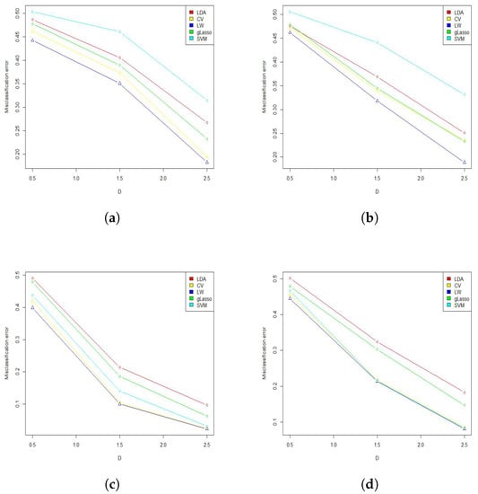
Figure 1. Misclassification error by increasing the Mahalanobis distance. (a) Mod1, $\rho =0.2,n=10$; (b) Mod1, $\rho =0.4,n=10$; (c) Mod2, $\rho =0.2,n=10$; (d) Mod2, $\rho =0.4,n=10$.

Figure 2 depicts the misclassification error for varying sample sizes. Not surprisingly, as n increased, the misclassification error decreased for all the methods in this study, but surprisingly, none of the methods had a smaller error compared to the LW. As shown in Figure 2, with the increasing sample size, the misclassification error in all methods was higher than the proposed method. Moreover, as the Mahalanobis distance increased, it became easier to identify which population the new observation $x^{*}$ belonged to, which improved the classification in the proposed method.

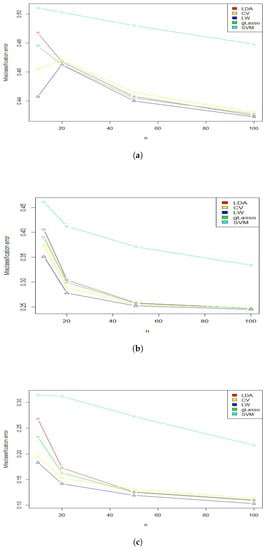
Figure 2. Misclassification error by increasing sample size and $p=12$. (a) Mod1, $\rho =0.2,D=0.5$; (b) Mod1, $\rho =0.2,D=1.5$; (c) Mod1, $\rho =0.2,D=2.5$.

To evaluate the efficiency of the LW method, simulations were performed using $p=16, 30, 50, 100, 500$ values. These results are summarized in Table 3. As the dimension increased, the classical method of linear discriminant analysis as well as the proposed cross-validation method of Mkhaderi [19] could not be used due to the singularity of the covariance matrix. With an increase in the value of $\mathit{D}$, the misclassification error decreased, and for each value $\mathit{D}$, the shrinkage method of LW was significantly better than the other methods.

Table 3. Misclassification error and shrinkage parameter values for $\rho =0.4$ in Mod1 state.

		LDA	CV	LW	gLasso	SVM
$\mathit{D}=0.5$	$p=12$	$0.475\left(0.072\right)$	$0.472\left(0.052\right)$	$\mathbf{0.462}\left(\mathbf{0.070}\right)$	$0.479\left(0.072\right)$	$0.506\left(0.034\right)$
	$p=16$	$0.494\left(0.060\right)$	$0.494\left(0.042\right)$	$\mathbf{0.450}\left(\mathbf{0.050}\right)$	$0.477\left(0.054\right)$	$502\left(0.050\right)$
	$p=30$	$---$a	$---$	$\mathbf{0.478}\left(\mathbf{0.066}\right)$	$0.495\left(0.076\right)$	$0.511\left(0.030\right)$
	$p=50$	$---$	$---$	$\mathbf{0.470}\left(\mathbf{0.063}\right)$	$0.493\left(0.061\right)$	$0.504\left(0.037\right)$
	$p=100$	$---$	$---$	$\mathbf{0.496}\left(\mathbf{0.045}\right)$	$0.504\left(0.039\right)$	$0.515\left(0.034\right)$
	$p=500$	$---$	$---$	$\mathbf{0.502}\left(\mathbf{0.044}\right)$	$0.519\left(0.056\right)$	$0.505\left(0.034\right)$
$\mathit{D}=1.5$	$p=12$	$0.369\left(0.055\right)$	$0.340\left(0.043\right)$	$\mathbf{0.318}\left(\mathbf{0.034}\right)$	$0.345\left(0.046\right)$	$0.441\left(0.057\right)$
	$p=16$	$0.413\left(0.077\right)$	$0.537\left(0.098\right)$	$\mathbf{0.334}\left(\mathbf{0.049}\right)$	$0.373\left(0.074\right)$	$0.458\left(0.045\right)$
	$p=30$	$---$	$---$	$\mathbf{0.372}\left(\mathbf{0.041}\right)$	$0.410\left(0.070\right)$	$0.501\left(0.053\right)$
	$p=50$	$---$	$---$	$\mathbf{0.409}\left(\mathbf{0.073}\right)$	$0.417\left(0.061\right)$	$0.490\left(0.037\right)$
	$p=100$	$---$	$---$	$\mathbf{0.415}\left(\mathbf{0.055}\right)$	$0.422\left(0.040\right)$	$0.502\left(0.027\right)$
	$p=500$	$---$	$---$	$\mathbf{0.451}\left(\mathbf{0.059}\right)$	$0.462\left(0.038\right)$	$0.518\left(0.027\right)$
$\mathit{D}=2.5$	$p=12$	$0.251\left(0.060\right)$	$0.235\left(0.068\right)$	$\mathbf{0.189}\left(\mathbf{0.045}\right)$	$0.233\left(0.057\right)$	$0.332\left(0.087\right)$
	$p=16$	$0.338\left(0.072\right)$	$0.592\left(0.115\right)$	$\mathbf{0.213}\left(\mathbf{0.054}\right)$	$0.260\left(0.057\right)$	$0.391\left(0.078\right)$
	$p=30$	$---$	$---$	$\mathbf{0.235}\left(\mathbf{0.062}\right)$	$0.276\left(0.070\right)$	$0.410\left(0.079\right)$
	$p=50$	$---$	$---$	$\mathbf{0.266}\left(\mathbf{0.055}\right)$	$0.286\left(0.061\right)$	$0.466\left(0.051\right)$
	$p=100$	$---$	$---$	$\mathbf{0.326}\left(\mathbf{0.067}\right)$	$0.330\left(0.053\right)$	$0.482\left(0.044\right)$
	$p=500$	$---$	$---$	$\mathbf{0.428}\left(\mathbf{0.069}\right)$	$0.430\left(0.076\right)$	$0.488\left(0.061\right)$

^a The covariance matrix is singular.

3.2. Real Data Analyses

In this section, we assess the performance of the five methods in classification for the datasets in Table 4.

Table 4. Datasets (Accessed on 30 November 2022).

	$\mathit{DataName}$	$\mathit{Specification}$	$\mathit{Link}$
Data1	$\mathit{BreastCancer}$	$\mathit{n}=116$	www.UCIMachineLearning.com
		$\mathit{p}=10$
Data2	$\mathit{Insurance}$	$\mathit{n}=36,634$	www.Kaggle.com
		$\mathit{p}=17$
Data3	$\mathit{LSVT}$	$\mathit{n}=126$	www.UCIMachineLearning.com
		$\mathit{p}=309$
Data4	$\mathit{mRNA}$	$\mathit{n}=219$	www.UCIMachineLearning.com
		$\mathit{p}=1650$

As shown in Table 5, the LW shrinkage method for classification was superior comparatively (marked as bold). In Data 4, the execution time in the system with specifications $CPU$: $i7-4720HQ$ and $Ram$: $8GB$ for the gLasso method took more than 10 h, and for the LW method it was less than 5 min, which was a sign of the rapidity of the shrinkage method in the classification of high-dimensional data.

Table 5. Misclassification error for the real datasets in Table 4.

	LDA	CV	SVM	gLasso	LW
Data1	$0.31707$	$0.26829$	$0.34146$	$0.29268$	$\mathbf{0.26829}$
Data2	$0.00063$	$0.00063$	$0.00009$	$0.00018$	$\mathbf{0.00009}$
Data3	$NaN$a	$NaN$	$0.21053$	$0.18421$	$\mathbf{0.10526}$
Data4	$NaN$	$NaN$	$0.00000$	$0.00000$	$\mathbf{0.00000}$

^a The covariance matrix is singular.

Figure 3 depicts the average of misclassification errors for the five methods, discussed in the paper.

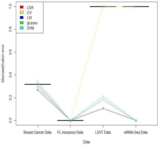
Figure 3. Misclassification error for the four real datasets.

4. Discussion and Conclusions

In the present paper, we aimed to improve the efficiency of the LDA classification method in high-dimensional situations, where the singularity of the inverse covariance matrix produced problems. We proposed to estimate the precision matrix with the shrinkage approach of Ledoit and Wolf (LW) [25], where the sample covariance matrix and a target matrix were linearly combined through a penalty factor in LDA classification.

The implementation of the suggested method on simulation data showed that for different scenarios, the proposed approach was superior to two powerful competitors, gLasso and SVM, in the sense of misclassification error. By increasing the Mahalanobis distance and using $p=100$ and $p=500$, we became more confident that the LW method could be considered as an alternative to some well-known methods for better classification.

In the real data analyses, three results were considerable. First, the analysis of Data1 and Data2 showed that LW was as good as the other competitors or much better when $n>>p$. Second, the misclassification of Data3 ($n=126, p=309$) exhibited that our method was more reliable than the others in high-dimensional regimes ($n<p$). Third, the LW method had the same misclassification error for Data4 when $n<<p$, compared to others. However, the execution time of the LW method was much shorter. In addition to high accuracy, the LW method was strongly recommended from the computation burden point of view, especially in a high-dimensional setting, where computing precision matrix estimation is challenging.

Lastly, if the covariance matrices of the populations are not the same (${\mathbf{\Sigma }}_i\ne {\mathbf{\Sigma }}_j;i,j=1,2,\dots ,K$), instead of LDA, it is possible to use the quadratic discriminant analysis (QDA). Friedman [31] proposed the method of regularized discriminant analysis (RDA) by using the trace estimator, $p^{-1}tr\left({\mathbf{\Sigma }}_{\mathbf{i}}\right){\mathbf{I}}_p$, and applying twice the shrinking sample covariance matrix. Since the trace estimator pools the diagonal elements of sample covariance matrices and ignores off-diagonal elements, Wu et al. [32] introduced the ppQDA estimator, which pools all elements in the covariance matrix, and it does not need to impose sparse assumptions. Although the ppQDA method has good asymptotic properties, it may not have a good performance for data classification. Therefore, considering (5) and Friedman’s [31] method as follows

$${\mathbf{S}}_i(\lambda ,\gamma )=(1-\gamma ){\mathbf{S}}_i\left(\lambda \right)+\gamma \left(p^{-1}tr\left({\mathbf{S}}_i\left(\lambda \right)\right){\mathbf{I}}_p\right),$$

where $\lambda$, $\gamma$ are tuning parameters, and ${\mathbf{S}}_i\left(\lambda \right)=\frac{(1-\lambda )(n_i-1){\mathbf{S}}_i+\lambda (n_1+n_2-2)\mathbf{S}}{(1-\lambda )(n_i-1)+\lambda (n_1+n_2-2)}$, it seems that by using the shrinkage method presented in this article, estimation of ${\mathbf{\Sigma }}_i$ can be improved and it is possible to reduce the misclassification error of high-dimensional data in the quadratic discriminant analysis mode.

References

- Clemmensen, L.; Hastie, T.; Witten, D.; Ersbøll, B. Sparse discriminant analysis. Technometrics 2011, 53, 406–413. [Google Scholar] [CrossRef]
- Peck, R.; Van Ness, J. The use of shrinkage estimators in linear discriminant analysis. IEEE Trans. Pattern Anal. Mach. Intell. 1982, 5, 530–537. [Google Scholar] [CrossRef] [PubMed]
- Srivastava, M.S. Multivariate theory for analyzing high dimensional data. J. Jpn. Stat. Soc. 2007, 37, 53–86. [Google Scholar] [CrossRef]
- Dempster, A.P. Covariance selection. Biometrics 1972, 28, 157–175. [Google Scholar] [CrossRef]
- Meinshausen, N.; Bühlmann, P. High-dimensional graphs and variable selection with the lasso. Ann. Stat. 2006, 34, 1436–1462. [Google Scholar] [CrossRef]
- Banerjee, O.; El Ghaoui, L.; d’Aspremont, A. Model selection through sparse maximum likelihood estimation for multivariate Gaussian or binary data. J. Mach. Learn. Res. 2008, 9, 485–516. [Google Scholar]
- Friedman, J.; Hastie, T.; Tibshirani, R. Sparse inverse covariance estimation with the graphical lasso. Biostatistics 2008, 9, 432–441. [Google Scholar] [CrossRef]
- Bickel, P.J.; Levina, E. Covariance regularization by thresholding. Ann. Stat. 2008, 36, 2577–2604. [Google Scholar] [CrossRef]
- Cai, T.T.; Zhang, L. High dimensional linear discriminant analysis: Optimality, adaptive algorithm and missing data. J. R. Stat. Soc. Ser. (Stat. Methodol.) 2019, 89, 675–705. [Google Scholar]
- Rothman, A.J.; Levina, E.; Zhu, J. Generalized thresholding of large covariance matrices. J. Am. Stat. Assoc. 2009, 104, 177–186. [Google Scholar] [CrossRef]
- Bien, J.; Tibshirani, R. Sparse estimation of a covariance matrix. Biometrika 2011, 98, 807–820. [Google Scholar] [CrossRef] [PubMed]
- Fan, J.; Liao, Y.; Liu, H. An overview of the estimation of large covariance and precision matrices. Econom. J. 2016, 19, C1–C32. [Google Scholar] [CrossRef]
- Stein, C.; James, W. Estimation with quadratic loss. In Proceedings of the Berkeley Symposium on Mathematical Statistics and Probability, Berkeley, CA, USA, 20–30 June 1961; Volume 1, pp. 361–379. [Google Scholar]
- Efron, B. Biased versus unbiased estimation. Adv. Math. 1975, 16, 259–277. [Google Scholar] [CrossRef]
- Efron, B.; Morris, C. Data analysis using Stein’s estimator and its generalizations. J. Am. Stat. Assoc. 1975, 70, 311–319. [Google Scholar] [CrossRef]
- Efron, B.; Morris, C. Multivariate empirical Bayes and estimation of covariance matrices. Ann. Stat. 1976, 4, 22–32. [Google Scholar] [CrossRef]
- Di Pillo, P.J. The application of bias to discriminant analysis. Commun. Stat. Theory Methods 1976, 5, 843–854. [Google Scholar] [CrossRef]
- Campbell, N.A. Shrunken estimators in discriminant and canonical variate analysis. J. R. Stat. Soc. Ser. (Appl. Stat.) 1980, 29, 5–14. [Google Scholar] [CrossRef]
- Mkhadri, A. Shrinkage parameter for the modified linear discriminant analysis. Pattern Recognit. Lett. 1995, 16, 267–275. [Google Scholar] [CrossRef][Green Version]
- Choi, Y.-G.; Lim, J.; Roy, A.; Park, J. Fixed support positive-definite modification of covariance matrix estimators via linear shrinkage. J. Multivar. Anal. 2019, 171, 234–249. [Google Scholar] [CrossRef]
- Bickel, P.J.; Levina, E. Regularized estimation of large covariance matrices. Ann. Stat. 2008, 36, 199–227. [Google Scholar] [CrossRef]
- Khare, K.; Rajaratnam, B. Wishart distributions for decomposable covariance graph models. Ann. Stat. 2011, 39, 514–555. [Google Scholar] [CrossRef]
- Cai, T.; Zhou, H. Minimax estimation of large covariance matrices under ℓ1-norm. Stat. Sin. 2012, 22, 1319–1349. [Google Scholar]
- Maurya, A. A well-conditioned and sparse estimation of covariance and inverse covariance matrices using a joint penalty. J. Mach. Learn. Res. 2016, 17, 4457–4484. [Google Scholar]
- Ledoit, O.; Wolf, M. A well-conditioned estimator for large-dimensional covariance matrices. J. Multivar. Anal. 2004, 88, 365–411. [Google Scholar] [CrossRef]
- Wang, C.; Pan, G.; Tong, T.; Zhu, L. Shrinkage estimation of large dimensional precision matrix using random matrix theory. Stat. Sin. 2015, 25, 993–1008. [Google Scholar] [CrossRef][Green Version]
- Hong, Y.; Kim, C. Recent developments in high dimensional covariance estimation and its related issues, a review. J. Korean Stat. Soc. 2018, 47, 239–247. [Google Scholar] [CrossRef]
- Le, K.T.; Chaux, C.; Richard, F.; Guedj, E. An adapted linear discriminant analysis with variable selection for the classification in high-dimension, and an application to medical data. Comput. Stat. Data Anal. 2020, 152, 107031. [Google Scholar] [CrossRef]
- Srivastava, M.S. Some tests concerning the covariance matrix in high dimensional data. J. Jpn. Stat. Soc. 2005, 35, 251–272. [Google Scholar] [CrossRef]
- Ledoit, O.; Wolf, M. Nonlinear shrinkage estimation of large-dimensional covariance matrices. Ann. Stat. 2012, 40, 1024–1060. [Google Scholar] [CrossRef]
- Friedman, J.H. Regularized discriminant analysis. J. Am. Stat. Assoc. 1989, 88, 165–175. [Google Scholar] [CrossRef]
- Wu, Y.; Qin, Y.; Zhu, M. Quadratic discriminant analysis for high-dimensional data. Stat. Sin. 2019, 29, 939–960. [Google Scholar] [CrossRef]
Publisher’s Note: MDPI stays neutral with regard to jurisdictional claims in published maps and institutional affiliations. |
© 2022 by the authors. Licensee MDPI, Basel, Switzerland. This article is an open access article distributed under the terms and conditions of the Creative Commons Attribution (CC BY) license (https://creativecommons.org/licenses/by/4.0/).