Abstract
Conventional Noise Clustering (NC) algorithms do not consider any spatial information in the image. In this study, three algorithms have been presented, Noise Local Information c-means (NLICM) and Adaptive Noise Local Information c-Means (ADNLICM), which use NC as the base classifier, and Noise Clustering with constraints (NC_S), which incorporates spatial information into the objective function of the NC classifier. These algorithms enhance the performance of classification by minimizing the effect of noise and outliers. The algorithms were tested on two study areas, Haridwar (Uttarakhand) and Banasthali (Rajasthan) in India. All three algorithms were examined using different parameters (distance measures, fuzziness factor, and δ). An analysis determined that the ADNLICM algorithm with Bray–Curtis distance measures, fuzziness factor m = 1.1, and δ = 106, outperformed the other algorithm and achieved 91.53% overall accuracy. The optimized algorithm returned the lowest variance and RMSE for both study areas, demonstrating that the optimized algorithm works for different satellite images. The optimized technique can be used to categorize images with noisy pixels and heterogeneity for various applications, such as mapping, change detection, area estimation, feature recognition, and classification.
MSC:
62H30; 94D05
1. Introduction
Image classification plays a vital role in remote sensing research because classification results are primary for many applications. To improve classification accuracy, many researchers and practitioners have introduced novel classification approaches and techniques [1]. Image classification is mainly done either as hard or soft classification. In hard classification techniques, one pixel belongs to a single class, which is impossible for a real scenario. An image may contain mixed pixels in a real scenario, which means one pixel may have multiple and partial class membership values. Fuzzy clustering algorithms are mainly designed to handle mixed pixels. Fuzzy c-means (FCM) [2], Possibilistic c-means (PCM) [3], and Noise Clustering (NC) [4] are the primary classifiers used for mixed pixel classification. FCM is a clustering method that allows one sample of data to assign a membership degree function to two or more clusters [5]. FCM is the first and most powerful method used in image classification. FCM was first developed in 1973 by Dunn [6] and further modified by Bezdek (1981). It is based on the minimization of an objective function and has been used for clustering, feature analysis, and target recognition. Pixel-based classification algorithms allot a pixel to a region based on similarities of spectral signature [7]. FCM does not consider information about the immediate neighborhood pixel, so it does not fully utilize the spatial information characteristics [8,9]. Ahmed et al. proposed Fuzzy c-means with constraints (FCM_S) [9]; in this algorithm, FCM combined with spatial information permits the labels in a pixel’s immediate neighborhood to affect its labeling. However, FCM_S is limited to single feature inputs [10]. To overcome the problem of FCM_S, [11] introduced the Fuzzy Local Information c-Means (FLICM) algorithm. A new factor was added to FLICM, incorporating both local- and gray-level information to control the neighborhood pixel effect and preserve the image details. Further, Zhang et al. proposed the Adaptive Fuzzy Local Information c-Means (ADFLICM) [12] algorithm to overcome the limitation of the FLICM algorithm. Zheng et al. proposed the generalized hierarchical fuzzy c-means algorithm [13] to solve the issue which comes from the outliers and Euclidean distance measures. Ding et al. proposed Kernel-based fuzzy c-means [14] to improve the clustering performance. Guo et al. designed an FCM-based framework to enhance the performance of noisy image segmentation by applying the filter [15]. Xu et al. suggested an intuitionistic fuzzy c-means (IFCM) algorithm that handles the uncertainty but does not correctly handle the noise [16]. To make IFCM handle the noise Verma et al. proposed improved intuitionistic fuzzy c-means (IIFCM) [17].
Some previous studies used contextual information using local convolutional techniques with FCM and PCM as base classifiers. In the current study, we have similarly used NC as a base classifier to incorporate contextual information in local convolutional methods to produce our three proposed algorithms, Noise Local Information c-Means (NLICM), Adaptive Noise Local Information c-Means (ADNLICM), and Noise Clustering with constraints (NC_S). The proposed algorithms may be utilized to prepare land-use land cover maps, which will be useful in agricultural mapping, hazard mapping, and other fields where a highly accurate LULC map is required [18,19,20,21]. FLICM, ADFLICM, FCM_S, Possibilistic c-means with constraints (PCM_S), Possibilistic Local Information c-Means (PLICM), Adaptive Possibilistic Local Information c-Means (ADPLICM) [22], Modified Possibilistic c-Means with constraints (MPCM-S) [23] are able to handle the noisy pixel problem; however, these were not tested for handling heterogeneity and different distance measures. Heterogeneity handling has now become an essential step in the classification process. To overcome this problem, this paper introduces three novel algorithms NLICM, ADNLICM, and NC_S, which are inspired by the FLICM, ADFLICM, and FCM_S algorithms, respectively. The FCM_S, FLICM, and ADFLICM algorithms are, in turn, based on the FCM algorithm, and the FCM algorithm is sensitive to noisy data and outliers [24]. To resolve the problem of this limitation of FCM, Dave and Sen (1993) introduced the Noise Clustering (NC) algorithm, which uses a new parameter delta (δ), known as “noise distance”.
The aim of this paper was to design and analyze NC-based local convolutional algorithms concerning different parameters to classify the satellite images, which handle the noisy and heterogeneous pixels. This paper proposed three NC-based algorithms, NLICM, ADNLICM, and NC_S, for handling noisy pixels and heterogeneity. These algorithms were first analyzed concerning different distance measures and important parameters (δ, m) of NC-based classifiers to obtain the best values by comparing the overall accuracy obtained by (FERM). Secondly, to check the performance of the algorithms, first, the variance was calculated to show that the optimized algorithm handles the heterogeneity correctly, and second, different degrees of random noise (1, 3, 5, 7, and 9%) were inserted in images of two sites (Haridwar and Banasthali) and the images classified by the optimized algorithm to confirm that the algorithm is suitable for handling noisy pixels. The paper is organized into four sections. Section 1 provides the background of the problem, a discussion of the different algorithms, and the aim of this study. Section 2 describes the Materials (study area and algorithms) and Methodology used in this paper. Section 3 explain the obtained results and their discussion. Finally, Section 4 summarizes the conclusions of the study.
2. Materials and Methods
2.1. Mathematical Concept of Classifiers
This section explains the mathematical principles behind the NC classifier’s use of spectral pixel-based information as well as the additional spatial local information added via the convolution approach. The algorithms Noise Local Information c-Means (NLICM), Adaptive Noise Local Information c-Means (ADNLICM), and Noise Clustering with Constraints (NC_S) have added local spatial information.
2.1.1. NC Classifier
The idea of Noise Clustering was suggested to handle the noise in a given dataset [25]. In this approach, noise is defined as a separate class and denoted by a parameter that consists of a constant distance, known as noise distance (δ), from all the data points. This algorithm is derived from the standard K-means algorithm. NC is generally used for building FCM and related robust algorithms. The NC algorithm is obtained using the following steps.
- Assign the means for each class and the value of the fuzziness factor (m).
- Compute the noise distance (δ) using Equation (1).
- Calculate the membership value () and mean cluster center () from Equation (2) and Equation (3), respectively;
- Assign the final class to each pixel.
Here, m = fuzziness factor (consisting of real values > 1), = degree of membership of ith pixel for cluster k, = ith d-dimensional measured data, = mean value (cluster center) of the kth class, = mean value (cluster center) of the jth class, N = total no of a pixel in the image, C = number of classes, δ = noise distance, = distance between and , = distance between and and = distance between and , define the objective function of the algorithms (NC, NLICM, ADNLICM, and NC_S), and represents the multiplier used to calculate δ from the average distances.
2.1.2. Noise Local Information c-Means (NLICM)
In this section, the NLICM algorithm is described. NLICM uses the neighborhood pixel to reduce the noisy pixel. It incorporates gray level and local spatial information into the objective function of the NC algorithm and the parameter, which was introduced by Krinidis and Chatzis (2010) in the FCM classifier. In this paper parameter is applied in the NC classifier, as the NC classifier handles noisy pixels better than the FCM classifier. The NLICM algorithm was obtained using the following steps.
- Assign the no of cluster (c) and fuzziness factor (m).
- Compute the δ parameter from Equation (1) and fuzzy factor () from Equation (5).
- Compute a new cluster applying Equation (6).
- Calculate the value of membership (Equation (7)).
- Assign the final class to each pixel.
The objective functions of NLICM, as mentioned in Equation (8), after applying function in the objective function of NC can be calculated from:
2.1.3. Adaptive Noise Local Information c-Means (ADNLICM)
This algorithm incorporates a local similarity measure in the image as well as a pixel spatial attraction model between pixels. According to Zhang et al. (2017), the local similarity measure in ADFLICM is based on the pixel spatial attraction model, which adaptively determines the weighting components for nearby pixels, similar to the way we used it for the NC- based fuzzy classifier on image feature enhancement. The objective function of ADNLICM is given in Equation (13). It uses local similarity measures (). The ADNLICM algorithm was obtained using the following steps.
- For each class, assign mean values.
- Assign the local window size, the fuzziness factor (m), and the no of class (c).
- Determine the noise distance (δ) using Equation (1) and the local similarity measure Sir using Equations (9) and (10).
Here, = pixel is the neighborhood pixel that falls into Ni, = pixel spatial attraction, and = spatial distance between i and r pixel.
- 4.
- Generate the final membership () and cluster mean () matrix using Equation (11) and Equation (12), respectively.
- 5.
- Assign each pixel to a final class.
ADNLICM integrates local spatial- and gray-level information into NC’s objective function. The objective function of ADNLICM is shown in Equation (13).
The objective function in Equation (13) was minimized to provide the membership function (Equation (11)).
2.1.4. Noise Clustering with Constraints (NC_S)
The NC_S algorithm is motivated by Fuzzy Clustering with Constraints (FCM_S) which was proposed by Ahmed et al. [26]. FCM_S introduces a new term into the standard FCM algorithm. This new term permits pixel labeling to be impacted by neighborhood labels. This paper used a new term in the NC classifier in place of the FCM classifier to handle the noise and heterogeneity. The computation steps for this algorithm are as follows.
- Assign the means for each class and the fuzziness factor (m).
- Compute the noise distance (δ) using Equation (1).
- The computation of the membership partition matrix () and the cluster centers are performed as follows () from Equation (14) and Equation (15), respectively;
Here,
= edge of the average value of the gray level over the within a window, = cardinality, a = parameter (control the effect of the neighbor term), and = represent the neighbor of .
- 4.
- Assign the final class to each pixel.
The NC_S algorithm objective function is derived as Equation (16).
2.2. Mathematical Formula of Similarity and Dissimilarity Measures
Two similarity metrics, Cosine, and Correlation, and eight dissimilarity measures, including Bray–Curtis, Canberra, Chessboard, Euclidean, Manhattan, Mean Absolute Difference, Median Absolute Difference, and Normalized Square Euclidean, have been utilized. Different measures of similarity and dissimilarity were investigated in fuzzy classifiers as distance criteria to be constructed to identify to which class unknown vectors belong. In this study, the most widely used distance metrics across several applications were chosen for investigation. The various distance measures were utilized to test and evaluate the models and to see how they affected the fuzzy classifier algorithm that was the subject of this study. All the dissimilarity and similarity measures’ mathematical expressions are given below. Here, c is the mean value, b is the number of bands, and x and v are the vector pixels. The different distance measures described in [27] are used in this study.
2.2.1. Bray–Curtis
The Bray–Curtis [28] dissimilarity is used to determine the connection between environmental sciences, ecology, and related fields. Bray–Curtis distance has the convenient property of having a value between 0 and 1. The same coordinate is represented by zero Bray–Curtis. The equation for Bray–Curtis is given in Equation (17). Figure 1 illustrates how Bray–Curtis distance works.
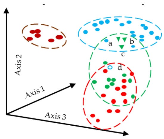
Figure 1.
Schematic Diagram of Bray–Curtis Distance Measures, a–d represents the sampling point.
Here N represents the no of data points, and y is the sample.
2.2.2. Canberra
The Canberra [29] measure is mainly applied to positive values. It analyses the total amount of fractional discrepancies between two objects’ coordinates. It has been employed to compare ranked lists and for intrusion detection in computer security. The equation for Canberra distance measures is given in Equation (18).
2.2.3. Chessboard
Chessboard [30] distance measures operate as a vector space to determine the greatest distance along two vectors between any two coordinate dimensions. It is also referred to as the Chebyshev distance. Equation (19) provides the formula for the distance on a chessboard. The concept of chessboard distance is shown in Figure 2.
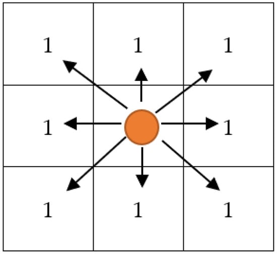
Figure 2.
Schematic Diagram of Chessboard Distance Measures.
2.2.4. Correlation
Correlation [31] similarity is a calculation that determines the correlation between two vectors. The Pearson-r correlation is used to determine how similar the two vectors are. With a perfect positive correlation at +1 and a perfect negative correlation at −1, its value ranges from −1 to +1, with 0 representing no correlation. Equation (20) contains the correlation’s mathematical formula. Figure 3 depicts the correlation distance idea.
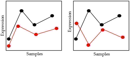
Figure 3.
Schematic Diagram of Correlation Distance Measures.
2.2.5. Cosine
Cosine [32] similarity measurements compute the cosine of an angle along two vectors in an inner product space. They provide the distance between two vectors as measured. Equation (21) contains the mathematical equation for Cosine similarity. Figure 4 depicts the cosine distance approach.
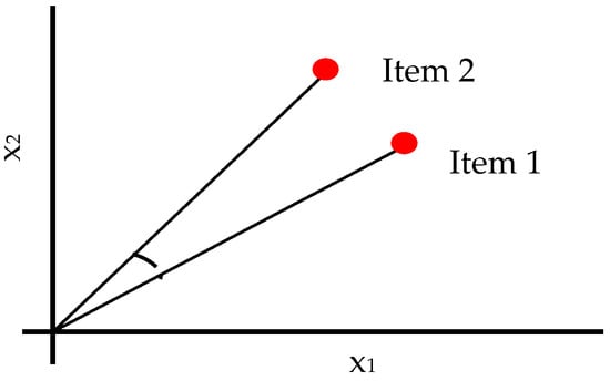
Figure 4.
Schematic Diagram of Cosine Distance Measures.
2.2.6. Euclidean
Two points in Euclidean space are separated by the Euclidean distance [30]. It computes the square root of the value difference between parallel data points as the sum of squares. Equation (22) contains the equation for Euclidean distance measures.
2.2.7. Manhattan
Images are compared using the Manhattan distance measures [33]. Manhattan distance is the product of the parallel element differences between any two data points. A small deviation from Euclidean distance is the Manhattan distance, which has a different formula for determining the separation between two data points. The Manhattan distance measures equation is given in Equation (23). The concepts of Euclidean and Manhattan distance are shown in Figure 5.
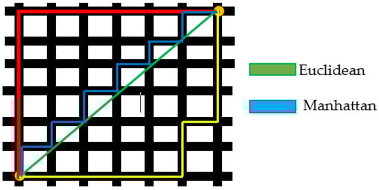
Figure 5.
Schematic Diagram of Euclidean and Manhattan Distance Measures.
2.2.8. Mean Absolute Difference
A statistical technique for depression is the Mean Absolute Difference [34]. It is determined by multiplying the total number of bands by the absolute difference between two things with similar locations in the same location and the variable between those two items. Equation (24) contains the formula for the Mean Absolute Difference in distance measurements. Figure 6 illustrates the idea of mean absolute difference distance.
Figure 6.
Schematic Diagram of Mean Absolute Difference Distance Measures.
2.2.9. Median Absolute Difference
To lessen the impact of impulsive noise on the derived measures, the median absolute difference (MAD) [35] may be used instead of the mean absolute difference. Mathematically generally, MAD is defined as finding the difference in the absolute brightness of the comparable pixels in two images before taking the data’s median. Equation (25) contains the equation for MAD distance measurements. Figure 7 illustrates the idea of median absolute difference distance.
Figure 7.
Schematic diagram of Median Absolute Difference Distance Measures.
2.2.10. Normalized Square Euclidean
The NSE distance between two vectors can be calculated using Normalized Square Euclidean (NSE) [33]. Before computing, the sum of the squared difference between the pixels of two images, the intensities of the pixels must first be normalized. Equation (26) contains the equation for NSE distance measurements.
2.3. Study Area and Dataset Used
This research work tested the NC algorithm and its versions in two study areas (site 1 and site 2). As shown in Figure 8, the first site considered was Haridwar (Uttarakhand). Site 1 was used to determine the optimized algorithm. The latitudes and longitudes covered by the first site are from 29°49′14″ to 29°52′21″ and 78°9′17″ to 78°13′4″, respectively. The coverage area is 5.92 km, east to west, and 5.95 km, north to south. Land-use diversity was the prime reason to choose this area; it helped examine and experiment with the convolutional method. The area includes water, wheat, dense forest, eucalyptus, grassland, and riverine sand. Landsat-8 and Formosat-2 satellite data were used in this study area; Table 1 shows the sensors’ specifications of Landsat-8, Formosat-2, and Sentinel-2 satellites.
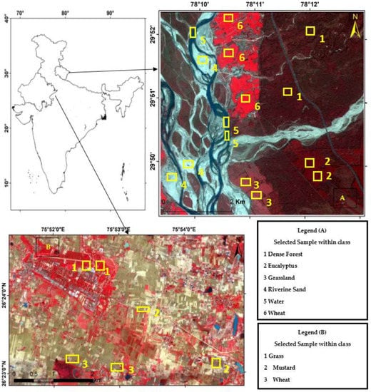
Figure 8.
Study Areas (A) Haridwar (Uttarakhand) (B) Banasthali (Rajasthan).

Table 1.
Specification of Landsat-8, Formosat-2, and Sentinel-2 [36,37].
The area surrounding Banasthali Vidyapith (Rajasthan) was selected as the second site area (Figure 8). This study area was used to classify the homogeneous classes by applying the optimized algorithm. The coverage area is situated in the northeastern region of Rajasthan, between latitudes 26°23′ and 26°24′ North and longitudes 75°51′ and 75°54′ East.
2.4. Methodology Adopted
Figure 9 shows the methodology and process flow adopted for this research work. This study’s primary focus has been on studying the conventional NC and proposed convolutional (NLICM, ADNLICM, and NC_S) classifiers. In addition, the influence of the delta (δ) and fuzziness factors, and various distance measures, on the proposed algorithm were studied using the two study areas (Haridwar and Banasthali). All algorithms were implemented in the JAVA environment through an in-house tool called SMIC (Sub-pixel Multi-spectral Image Classifier) [38]. The methodology was derived by the following steps.
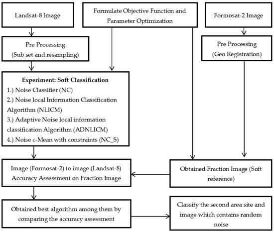
Figure 9.
Flow diagram of Adopted Methodology.
Step 1: Classify the image by NC classifier and local conventional NLICM, ADNLICM, and NC_S using NC as the base classifier employing various delta (δ), distance measures, and fuzziness factor parameters.
Step 2: Calculate the overall accuracy of the obtained classified image to determine the optimized parameters for the algorithm.
Step 3: Calculate the overall accuracy and compare all algorithms to find the best algorithm.
Step 4: Use the optimal proposed algorithm and NC classifier to classify the image with 1% (density = 0.01), 3% (density = 0.03), 5% (density = 0.05), 7% (density = 0.07), and 9% (density = 0.09), pepper and salt-and-pepper random noise to show that the proposed algorithms handle the noise correctly.
Step 5: Calculate the variance of the obtained optimal proposed algorithm and NC classifier to show that the proposed algorithm is better able to handle the heterogeneity than the NC classifier.
Step 6: Use the optimal proposed algorithm and NC classifier to classify the second study area (site 2) with (1, 3, 5, 7, and 9%) pepper and salt-and-pepper noise or without random noise to show that the proposed algorithm can also handle noise and heterogeneity with different images.
3. Results and Discussion
The result and discussion section are divided into five experiments. In the First Experiment, the optimized algorithm with respect to OA for the NC and NC base local convolutional classifier (NLICM, ADNLICM, and NC_S) is obtained while applying different parameters such as various distance measures, delta (δ), and fuzziness factor (m). The distance measures tested consist of Bray–Curtis, Canberra, Chessboard, Correlation, Cosine, Manhattan, Mean Absolute Difference, Median Absolute Difference, and Normalized Square Euclidean. Values of δ in the range 104 to 1013, with an interval of multiple of 10, and m values (1.1-3) with a period of 0.2, were considered. In the second experiment, the optimized algorithms were used to classify the Landsat-8 image containing 1%, 3%, 5%, 7%, or 9% pepper, and salt-and-pepper random noise.
In the third experiment, the NC and proposed algorithms were used to classify the Landsat-8 classes (Dense Forest, Eucalyptus, Grassland, Riverine Sand, Water, and Wheat) and calculate the OA and variance to confirm that the ADNLICM algorithm handles random heterogeneity better than the other algorithms. The fourth and fifth experiments are the same as the second and third, respectively, with a Sentinel-2 image used in place of the Landsat-8 image to show that the proposed algorithm also works on other satellite data and maps the homogeneous class (Mustard, Wheat, and Grassland) correctly.
3.1. Experiment 1: Compute the Optimized Algorithms
In this section, OA is computed using the FERM technique to obtain the optimized NC, NLICM, ADNLICM, and NC_S algorithms with respect to different distance measures and parameters. The best algorithm will be selected by comparison.
Figure 10 shows the different weighting components and overall accuracy for the NC classifier with various delta (δ), m, and distance measures. For δ = 104, Canberra distance measures delivered the highest OA (80.48%) at m = 1.1 (Figure 10a). At δ = 105, Mean Absolute Difference distance measures gave the best OA (77.22%) at m = 1.1 (Figure 10b). At δ = 106, Bray–Curtis distance measures, gave the highest OA (77.72%) at m = 1.1 (Figure 10c). At δ = 107, Bray–Curtis distance measures produced the highest OA (77.81%) at m = 1.1 (Figure 10d). At δ = 108, Canberra distance measures produced the highest OA (82.55%) at m = 1.1 (Figure 10e). At = 109, Mean Absolute Difference distance measures result in the highest OA (78.46%) at m = 1.1 (Figure 10f). At δ = 1010, Mean Absolute Difference distance measures delivered the highest OA (77.75%) at m = 1.1 (Figure 10d). At δ = 1011, Bray–Curtis distance measures, gave the highest OA (77.35%) at m = 1.1 (Figure 10g). At δ = 1012, Canberra distance measures gave the highest OA (81.33%) at m = 1.1 (Figure 10h). At δ = 1013, Mean Absolute Difference distance measures produced the most increased OA (78.30%) at m = 1.1 (Figure 10i).
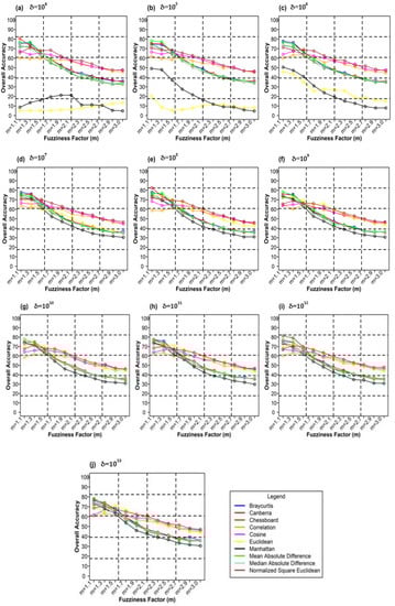
Figure 10.
Comparison of overall accuracy in NC classifier for applying different distance measures, m (1.1–3.0), and (a–j) for site 1 (Haridwar).
Figure 11 plots different weighting components and overall accuracy for various delta (δ) and distance measures for the NLICM classifier. At δ = 104, Canberra distance measures gave the highest OA (86.91%) at m = 1.1 (Figure 11a). For δ = 105, Bray–Curtis distance measures gave the highest OA (86.40%) at m = 1.1 (Figure 11b). For δ = 106, Canberra distance measures gave the highest OA (87.38%) at m = 1.1 (Figure 11c). At 107, Mean Absolute Difference distance measures produced the highest OA (87.80%) at m = 1.1 (Figure 11d). For δ = 108, Canberra distance measures gave the highest OA (88.75%) at m = 1.1 (Figure 11e). At δ = 109, the highest OA (89.50%) at m = 1.1 was achieved by Bray–Curtis distance measures (Figure 11f). At δ = 1010, Manhattan distance measures delivered the highest OA (88.45%) at m = 1.1 (Figure 11g). At δ = 1011, Manhattan distance measures gave the highest OA (88.35%) at m = 1.1 (Figure 11h). For δ = 1012, Euclidean distance measures gave the highest OA (88.47%) at m = 1.3 (Figure 11i). At δ = 1013, Canberra distance measures delivered the highest OA (87.40%) at m = 1.1 (Figure 11j).
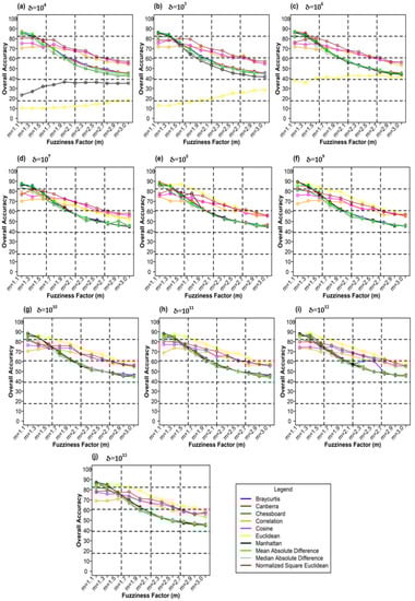
Figure 11.
Comparison of overall accuracy in NLICM classifier for applying different distance measures, m (1.1–3.0), and (a–j) for site 1 (Haridwar).
Figure 12 shows plots of the different weighting components and overall accuracy for various delta (δ) and distance measures for the ADNLICM classifier. For δ = 104, Mean Absolute Difference distance measures produced the highest OA (88.93%) at m = 1.1 Figure 12a). At δ = 105, Bray–Curtis distance measures gave the highest OA (89.45%) at m = 1.3 (Figure 12b). At δ = 106 Bray–Curtis distance measures delivered the highest OA (91.53%) at m = 1.1 (Figure 12c). At δ = 107, Mean Absolute Difference distance measures gave the highest OA (90.22%) at m = 1.3 (Figure 12d). At δ = 108 Mean Absolute Difference distance measures, produced the most increased OA (89.47%) at m = 1.3 (Figure 12e). For δ = 109, Manhattan distance measures made the most increased OA (90.22%) at m = 1.3 (Figure 12f). At δ = 1010, Mean Absolute Difference distance measures gave the highest OA (89.50%) at m = 1.3 (Figure 12g). At δ = 1011, Mean Absolute Difference distance measures gave the highest OA (89.33%) at m = 1.1 (Figure 12h). At δ = 1012, Bray–Curtis distance measures delivered the highest OA (88.90%) at m = 1.3 (Figure 12i). For δ = 1013, Manhattan distance measures gave the highest OA (89.94 %) at m = 1.3 (Figure 12j).
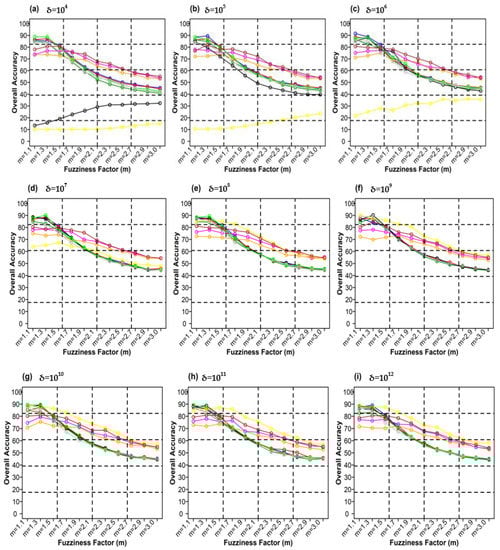
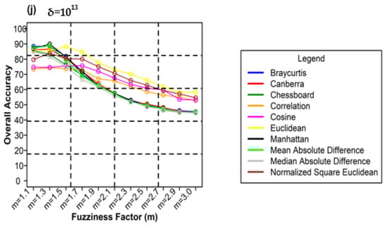
Figure 12.
Comparison of overall accuracy in ADNLICM classifier for applying different distance measures, m (1.1–3.0), and (a–j) for site 1 (Haridwar).
Figure 13 shows plots between different weighting components and overall accuracy for various delta (δ) and distance measures for the NC_S classifier. For δ = 104, Canberra distance measures gave the highest OA (87.70%) at m = 1.1 (Figure 13a). At δ = 105 Manhattan distance measures gave the highest OA (89.02%) at m = 1.1 (Figure 13b). At δ = 106, Bray–Curtis distance measures delivered the highest OA (89.36%) at m = 1.1 (Figure 13c). At δ = 107, Canberra distance measures gave the highest OA (89.43%) at m = 1.1 (Figure 13d). For δ = 108, Manhattan distance measures produced the highest OA (89.99%) at m = 1.1 (Figure 13e). At δ = 109, Bray–Curtis distance measures gave the highest OA (90.01%) at m = 1.1 (Figure 13f). At δ = 1010, Bray–Curtis distance measures delivered the highest OA (89.14%) at m = 1.1 (Figure 13g). At δ = 1011, Mean Absolute Difference distance measures produced the best OA (87.95%) at m = 1.1 (Figure 13g). For δ = 1012, Euclidean distance measures gave the best OA (88.00%) at m = 1.3 (Figure 13h). At δ = 1013, Manhattan distance measures gave the highest OA (89.28%) at m = 1.1 (Figure 13i).
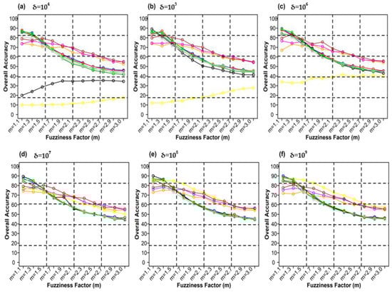
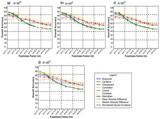
Figure 13.
Comparison of overall accuracy in NC_S classifier for applying different distance measures, m (1.1–3.0), and (a–j) for site 1 (Haridwar).
For the NC, NLICM, ADNLICM, and NC_S classifiers, Table 2, Table 3, Table 4 and Table 5 show the Kappa and RMSE calculated for the maximum overall accuracy (Shown in Figure 10, Figure 11, Figure 12 and Figure 13) observed with regard to various parameters.
Table 2.
Kappa and RMSE determined for the highest overall accuracy of the NC classifier by applying different parameters for site 1 (Haridwar).
Table 3.
Kappa and RMSE determined for the highest overall accuracy of the NLICM classifier by applying different parameters for site 1 (Haridwar).
Table 4.
Kappa and RMSE determined for the highest overall accuracy of the ADNLICM classifier by applying different parameters for site 1 (Haridwar).
Table 5.
Kappa and RMSE determined for the highest overall accuracy of the NC_S classifier by applying different parameters for site 1 (Haridwar).
3.2. Experiment 2: Classification in the Presence of Noise in the Haridwar Study Area Site
This experiment evaluated the effects of adding 1%, 3%, 5%, 7%, and 9% random noise in the form of pepper and salt-and-pepper to Landsat-8 images. The original image with 1%, 3%, 5%, 7%, and 9% additional pepper and salt-and-pepper noise is shown in Table 6 and Table 7, respectively. The difference between the original classified image and the noisy classified image is used to calculate the RMSE and FERM. Kappa is also calculated. To calculate FERM and RMSE, Formosat-2 images were utilized as the reference image. RMSE, FERM, and kappa results show (Table 8) that the ADNLICM classifier performs better than the other classifiers.
Table 6.
Landsat-8 original and dense forest classified class image with respect to different random pepper noise (for site 1 (Haridwar)).
Table 7.
Landsat-8 original and dense forest classified class image with respect to different random salt-and-pepper noise (for site 1 (Haridwar)).
Table 8.
RMSE, FERM, and Kappa of the algorithms concerning different random noise (pepper and salt-and-pepper noise) for site 1 (Haridwar).
Table 6 and Table 7 show the Landsat-8 image consisting of 1%, 3%, 5%, 7%, and 9% random pepper and salt-and-pepper noise in the original image and classified image of dense forest with NC, NLICM, NC_S, and ADNLICM algorithm, respectively.
Table 8 shows the calculated Root Mean Square Error (RMSE), FERM (Fuzzy Error Matrix), and Kappa value of the NC, NLICM, NC_S, and ADNLICM algorithms for the Dense Forest classified class with 1%, 3%, 5%, 7%, and 9% random pepper and salt-and-pepper noise. Pepper and salt-and-pepper noise give almost the same result. This result shows that the ADNLICM algorithm obtained a lower value for RMSE, FERM, and Kappa than the other algorithms. Thus, we conclude that the ADNLICM algorithm performs better in the presence of noise than the other algorithms.
3.3. Experiment 3: Classification Outputs of Haridwar Study Area Site to Calculate Variance and SSE
Table 9 shows the classified outputs of the NC, NLICM, NC_S, and ADNLICM algorithms. The green patches show the classified classes of dense forest, eucalyptus, grassland, sand, water, and wheat.
Table 9.
Classified classes for each algorithm for site 1 (Haridwar).
Table 10 shows the variance within the class for the NC, NLICM, NC_S, and ADNLICM algorithms. It was observed that the ADNLICM classifier provides the least variance value for all six classes. This result shows that the ADNLICM classification algorithm handles heterogeneity correctly.
Table 10.
Variance within the class for each algorithm for site 1 (Haridwar).
Next, we calculated the variance (Table 10) and Sum of Square Errors (SSE) (Table 11) of the classified outcomes of the Haridwar study area site using the proposed technique. Lower variance values demonstrate an algorithm’s ability to handle heterogeneity well. In contrast, lower SSE values reveal which algorithm performs the best clustering validation.
Table 11.
SSE values for the proposed algorithms for site 1 (Haridwar).
Table 11 shows SSE, used to show the cluster validity of the proposed algorithm, values. This cluster validity method comes under the relative approach. Table 12 again shows that the ADNLICM algorithm performed better than the other algorithms.
Table 12.
Sentinel-2 original and hard classified image for site 2 (Banasthali).
3.4. Experiment 4: Classification in the Presence of Noise in the Banasthali Study Area Site
This experiment assessed the impacts of 1%, 3%, 5%, 7%, and 9% pepper and salt-and-pepper-style random noise added to Sentinel-2 Landsat-8 images. Table 12 shows the Sentinel-2 image containing 1%, 3%, 5%, 7%, and 9% random pepper noise in the original image and hard classified image of the Sentinel-2 image shown after applying NLICM, NC_S, and ADNLICM algorithm.
The RMSE was calculated using the difference between the original classified image and the noisy classified image. FERM and Kappa were also calculated. To calculate FERM and RMSE, Sentinel-2 images were classified as hard and ERDAS Imagine Software was used. RMSE, FERM, and kappa result shows (Table 8) which classifier performs better compared to other classifiers.
Table 13 shows the evaluated overall accuracy (FERM), RMSE, and Kappa of the NC, NLICM, NC_S, and ADNLICM algorithms for hard classified images with 1%, 3%, 5%, 7%, and 9% random pepper noise. This result shows that the ADNLICM algorithm performed better than the other algorithms. Thus, it has been concluded that the ADNLICM algorithm performs better in the presence of noise than the other algorithms.
Table 13.
RMSE, FERM, and Kappa for each algorithm with different random noise (pepper) for site 2 (Banasthali).
3.5. Experiment 5: Classification Outputs of Banasthali Study Area Site to Calculate Variance
Table 14 shows the classified outputs of the NLICM, NC_S, and ADNLICM algorithms, to compare classified results and calculate the variance value. The green patches show the classified classes of Grass, Mustard, and Wheat.
Table 14.
Classified classes for site 1 (Haridwar).
This experiment calculates the variance (Table 15) for the Banasthali study Area site. Lower variance values show the robustness of an algorithm to heterogeneity.
Table 15.
Variance within the classes for the given algorithms for site 2 (Banasthali).
Table 15 shows the variance within the classes for the NC, NLICM, NC_S, and ADNLICM algorithms; it was seen that the ADNLICM classifier provides the least variance value for all three classes. This result shows that the ADNLICM classification algorithm handles heterogeneity well.
3.6. Discussion in Comparison with Other Studies
The present study focused on local convolutional information methods. Previous studies on this method used FCM and PCM-based classifiers, while the present study is based on NC classifiers. A comparison of maximum OA obtained in previous studies and the present work is shown in Table 16. The optimized algorithm achieved from this study was comparable with the other studies in terms of overall accuracy.
Table 16.
Comparison of OA with different studies.
The Markov Random Field (MRF (DA)) [41] approach requires optimization of the global energy function, which is very sensitive to handle, which ADNLICM does not require. The FLICM [27], ADPLICM [22], MPCM_S [40], and PLICM [39] algorithms studied the handling of noisy pixels utilizing FC and PCM as the base classifier. Whereas, in this research work, local convolution methods have been added to the NC classifier, resulting in increased OA. The ADNLICM algorithm provides good classification results in terms of noisy pixels and heterogeneity and provides the highest Overall Accuracy of 91.53%. All the compared studies were performed on the same Landsat-8 dataset and resolution; hence a logical comparison was performed in this study, and it is inferred from the analysis that the proposed algorithm improved the overall accuracy.
4. Conclusions
The conventional Noise Clustering (NC) algorithm does not incorporate spatial information. This research examined three novel NC-based algorithms, NLICM, ADNLICM, and NC_S, that consider spatial information to better handle noise and heterogeneity. This paper concentrated on obtaining an optimized algorithm concerning different parameters (distance measures, m, and δ). The optimum overall accuracy for the ADNLICM algorithm was found to be 91.53% for Bray–Curtis distance measures, fuzziness factor at (m) = 1.1, and δ = 106. The proposed algorithms with NC-based classifier tested using 1%, 3%, 6%, and 9% random noise (pepper, and salt-and-pepper) achieve the lowest value of RMSE, FERM, and kappa for the Dense Forest class using the ADNLICM algorithm, which shows that the proposed method handles noise effectively. For the optimized ADNLICM algorithm, the variance is also lower compared to the other classifiers. Further, in this research, the optimized ADNLICM algorithm was validated using the sentinel-2 data in terms of RMSE, kappa, and variance for handling noise and heterogeneity, respectively.
The previous work performed for the study area used FCM- and PCM-based classifiers; in this study, the NC classifier was used, which performs better than FCM and PCM in handling noise and heterogeneity. Previous works mainly studied two or three distance measures to calculate the accuracy; in this work, 10 different distance measures and parameters were utilized to calculate the accuracy; and it was found that overall accuracy improved substantially. The proposed algorithm preserves the boundaries of the different feature classes. The techniques may be used for various applications, including mapping, change detection, area estimation, feature recognition, and classification while handling noisy/isolated pixels.
Author Contributions
Conceptualization, S.S., A.K. and D.K.; methodology, S.S. and A.K.; software, S.S. and A.K.; validation, A.K., S.S. and D.K.; formal analysis, S.S.; writing—original draft preparation, S.S.; writing—review and editing, A.K. and D.K.; visualization, S.S.; supervision, A.K. and D.K. All authors have read and agreed to the published version of the manuscript.
Funding
This research received no external funding.
Data Availability Statement
Not applicable.
Conflicts of Interest
The authors declare no conflict of interest.
References
- Lillesand, T.; Kiefer, R.W.; Chipman, J. Remote Sensing and Image Interpretation; John Wiley & Sons: Hobokan, NJ, USA, 2014. [Google Scholar]
- Bezdek, J.C.; Ehrlich, R.; Full, W. FCM: The fuzzy c-means clustering algorithm. Comput. Geosci. 1984, 10, 191–203. [Google Scholar] [CrossRef]
- Krishnapuram, R.; Keller, J. A possibilistic approach to clustering. IEEE Trans. Fuzzy Syst. 1993, 1, 98–110. [Google Scholar] [CrossRef]
- Dave, R.; Sen, S. Noise Clustering Algorithm Revisited; IEEE: Piscataway, NZ, USA, 1997; pp. 199–204. [Google Scholar]
- Dagher, I.; Issa, S. Subband effect of the wavelet fuzzy C-means features in texture classification. Image Vis. Comput. 2012, 30, 896–905. [Google Scholar] [CrossRef]
- Dunn, J.C. A Fuzzy Relative of the ISODATA Process and Its Use in Detecting Compact Well-Separated Clusters. J. Cybern. 1973, 3, 32–57. [Google Scholar] [CrossRef]
- Chakraborty, D.; Singh, S.; Dutta, D. Segmentation and classification of high spatial resolution images based on Hölder exponents and variance. Geo-Spatial Inf. Sci. 2017, 20, 39–45. [Google Scholar] [CrossRef][Green Version]
- Yu, J.; Guo, P.; Chen, P.; Zhang, Z.; Ruan, W. Remote sensing image classification based on improved fuzzy c-means. Geo-spatial Inf. Sci. 2008, 11, 90–94. [Google Scholar] [CrossRef]
- Ahmed, M.; Yamany, S.; Farag, A.; Moriarty, T. Bias Field Estimation and Adaptive Segmentation of MRI Data Using a Modified Fuzzy C-Means Algorithm; IEEE: Piscataway, NZ, USA, 2003; pp. 1250–1255. [Google Scholar]
- Chuang, K.-S.; Tzeng, H.-L.; Chen, S.; Wu, J.; Chen, T.-J. Fuzzy c-Means clustering with spatial information for image segmentation. Comput. Med. Imaging Graph. 2006, 30, 9–15. [Google Scholar] [CrossRef]
- Krinidis, S.; Chatzis, V. A Robust Fuzzy Local Information C-Means Clustering Algorithm. IEEE Trans. Image Process. 2010, 19, 1328–1337. [Google Scholar] [CrossRef]
- Zhang, H.; Wang, Q.; Shi, W.; Hao, M. A Novel Adaptive Fuzzy Local Information C-Means Clustering Algorithm for Remotely Sensed Imagery Classification. IEEE Trans. Geosci. Remote Sens. 2017, 55, 5057–5068. [Google Scholar] [CrossRef]
- Zheng, Y.H.; Jeon, B.; Xu, D.H.; Wu, Q.M.J.; Zhang, H. Image segmentation by generalized hierarchical fuzzy C-means algorithm. J. Intell. Fuzzy Syst. 2015, 28, 961–973. [Google Scholar] [CrossRef]
- Ding, Y.; Fu, X. Kernel-Based fuzzy c-Means clustering algorithm based on genetic algorithm. Neurocomputing 2016, 188, 233–238. [Google Scholar] [CrossRef]
- Guo, L.; Chen, L.; Chen, C.P.; Zhou, J. Integrating guided filter into fuzzy clustering for noisy image segmentation. Digit. Signal Process. 2018, 83, 235–248. [Google Scholar] [CrossRef]
- Xu, Z.; Wu, J. Intuitionistic fuzzy C-means clustering algorithms. J. Syst. Eng. Electron. 2010, 21, 580–590. [Google Scholar] [CrossRef]
- Verma, H.; Agrawal, R.; Sharan, A. An improved intuitionistic fuzzy c-means clustering algorithm incorporating local information for brain image segmentation. Appl. Soft Comput. 2016, 46, 543–557. [Google Scholar] [CrossRef]
- Rawat, A.; Kumar, D.; Chatterjee, R.S.; Kumar, H. A GIS-based liquefaction susceptibility mapping utilising the morphotectonic analysis to highlight potential hazard zones in the East Ganga plain. Environ. Earth Sci. 2022, 81, 1–16. [Google Scholar] [CrossRef]
- Rawat, A.; Kumar, D.; Chatterjee, R.S.; Kumar, H. Reconstruction of liquefaction damage scenario in Northern Bihar during 1934 and 1988 earthquake using geospatial methods. Geomatics Nat. Hazards Risk 2022, 13, 2560–2578. [Google Scholar] [CrossRef]
- Zhang, D.; Pan, F.; Diao, Q.; Feng, X.; Li, W.; Wang, J. Seeding Crop Detection Framework Using Prototypical Network Method in UAV Images. Agriculture 2021, 12, 26. [Google Scholar] [CrossRef]
- Pant, N.; Dubey, R.K.; Bhatt, A.; Rai, S.P.; Semwal, P.; Mishra, S. Soil erosion and flood hazard zonation using morphometric and morphotectonic parameters in Upper Alaknanda river basin. Nat. Hazards 2020, 103, 3263–3301. [Google Scholar] [CrossRef]
- Singh, A.; Kumar, A.; Upadhyay, P. A novel approach to incorporate local information in Possibilistic c-Means algorithm for an optical remote sensing imagery. Egypt. J. Remote Sens. Space Sci. 2020, 24, 1–11. [Google Scholar] [CrossRef]
- Wu, X.H.; Zhou, J.J. Modified possibilistic clustering model based on kernel methods. J. Shanghai Univ. 2008, 12, 136–140. [Google Scholar] [CrossRef]
- Zhao, F. Fuzzy clustering algorithms with self-tuning non-local spatial information for image segmentation. Neurocomputing 2013, 106, 115–125. [Google Scholar] [CrossRef]
- Dave, R.; Krishnapuram, R. Robust clustering methods: A unified view. IEEE Trans. Fuzzy Syst. 1997, 5, 270–293. [Google Scholar] [CrossRef]
- Ahmed, M.; Yamany, S.; Mohamed, N.; Farag, A.; Moriarty, T. A modified fuzzy c-means algorithm for bias field estimation and segmentation of MRI data. IEEE Trans. Med. Imaging 2002, 21, 193–199. [Google Scholar] [CrossRef]
- Suman, S.; Kumar, D.; Kumar, A. Study the Effect of Convolutional Local Information-Based Fuzzy c-Means Classifiers with Different Distance Measures. J. Indian Soc. Remote Sens. 2021, 49, 1561–1568. [Google Scholar] [CrossRef]
- Bray, J.R.; Curtis, J.T. An Ordination of the Upland Forest Communities of Southern Wisconsin. Ecol. Monogr. 1957, 27, 325–349. [Google Scholar] [CrossRef]
- Agarwal, S.; Burges, C.; Crammer, K. Advances in Ranking. In Proceedings of the Twenty-Third Annual Conference on Neural Information Processing Systems, Whistler, BC, USA; 2009; pp. 1–81. [Google Scholar]
- Baccour, L.; John, R.I. Experimental analysis of crisp similarity and distance measures. In Proceedings of the 2014 6th International Conference of Soft Computing and Pattern Recognition (SoCPaR), Tunis, Tunisia, 11–14 August 2014; IEEE: Piscataway, NZ, USA, 2014; pp. 96–100. [Google Scholar]
- Székely, G.J.; Rizzo, M.L.; Bakirov, N.K. Measuring and testing dependence by correlation of distances. Ann. Stat. 2007, 35, 2769–2794. [Google Scholar] [CrossRef]
- Senoussaoui, M.; Kenny, P.; Stafylakis, T.; Dumouchel, P. A Study of the Cosine Distance-Based Mean Shift for Telephone Speech Diarization. IEEE/ACM Trans. Audio Speech Lang. Process. 2013, 22, 217–227. [Google Scholar] [CrossRef]
- Hasnat, A.; Halder, S.; Bhattacharjee, D.; Nasipuri, M.; Basu, D.K. Comparative Study of Distance Metrics for Finding Skin Color Similarity of Two Color Facial Images; ACER: New Taipei City, Taiwan, 2013; pp. 99–108. [Google Scholar]
- Vassiliadis, S.; Hakkennes, E.; Wong, J.; Pechanek, G. The sum-Absolute-Difference motion estimation accelerator. In Proceedings of the 24th EUROMICRO Conference (Cat. No. 98EX204), Vasteras, Sweden, 27 August 1998; IEEE: Piscataway, NZ, USA, 2002. [Google Scholar]
- Scollar, I.; Huang, T.; Weidner, B. Image enhancement using the median and the interquartile distance. In Proceedings of the 2018 IEEE International Conference on Multimedia and Expo (ICME), Boston, MA, USA, 14–16 April 1983; IEEE: Piscataway, NZ, USA, 1984. [Google Scholar]
- Nandan, R.; Kamboj, A.; Kumar, A.; Kumar, S.; Reddy, K.V. Formosat-2 with Landsat-8 Temporal -Multispectral Data for Wheat Crop Identification using Hypertangent Kernel based Possibilistic classifier. J. Geomat. 2016, 10, 89–95. [Google Scholar]
- Khamdamov, R.; Saliev, E.; Rakhmanov, K. Classification of crops by multispectral satellite images of sentinel 2 based on the analysis of vegetation signatures. J. Phys. Conf. Ser. 2020, 1441, 012143. [Google Scholar] [CrossRef]
- Kumar, A.; Upadhyay, P. Fuzzy Machine Learning Algorithms for Remote Sensing Image Classification; CRC Press: Boca Raton, FL, USA, 2020. [Google Scholar]
- Suman, S.; Kumar, A.; Kumar, D.; Soni, A. Augmenting possibilistic c-means classifier to handle noise and within class heterogeneity in classification. J. Appl. Remote Sens. 2021, 15, 1–17. [Google Scholar] [CrossRef]
- Singh, A.; Kumar, A.; Upadhyay, P. Modified possibilistic c-means with constraints (MPCM-S) approach for incorporating the local information in a remote sensing image classification. Remote Sens. Appl. Soc. Environ. 2020, 18, 100319. [Google Scholar] [CrossRef]
- Suman, S.; Kumar, D.; Kumar, A. Study the Effect of MRF Model on Fuzzy c Means Classifiers with Different Parameters and Distance Measures. J. Indian Soc. Remote Sens. 2022, 50, 1177–1189. [Google Scholar] [CrossRef]


Publisher’s Note: MDPI stays neutral with regard to jurisdictional claims in published maps and institutional affiliations. |
© 2022 by the authors. Licensee MDPI, Basel, Switzerland. This article is an open access article distributed under the terms and conditions of the Creative Commons Attribution (CC BY) license (https://creativecommons.org/licenses/by/4.0/).