Application of Computational Model Based Probabilistic Neural Network for Surface Water Quality Prediction

Abstract

Applications of artificial intelligence (AI) models have been massively explored for various engineering and sciences domains over the past two decades. Their capacity in modeling complex problems confirmed and motivated researchers to explore their merit in different disciplines. The use of two AI-models (probabilistic neural network and multilayer perceptron neural network) for the estimation of two different water quality indicators (namely dissolved oxygen (DO) and five days biochemical oxygen demand (BOD₅)) were reported in this study. The WQ parameters estimation based on four input modelling scenarios was adopted. Monthly water quality parameters data for the duration from January 2006 to December 2015 were used as the input data for the building of the prediction model. The proposed modelling was established utilizing many physical and chemical variables, such as turbidity, calcium (Ca), pH, temperature (T), total dissolved solids (TDS), Sulfate (SO₄), total suspended solids (TSS), and alkalinity as the input variables. The proposed models were evaluated for performance using different statistical metrics and the evaluation results showed that the performance of the proposed models in terms of the estimation accuracy increases with the addition of more input variables in some cases. The performances of PNN model were superior to MLPNN model with estimation both DO and BOD parameters. The study concluded that the PNN model is a good tool for estimating the WQ parameters. The optimal evaluation indicators for PNN in predicting BOD are (R² = 0.93, RMSE = 0.231 and MAE = 0.197). The best performance indicators for PNN in predicting Do are (R² = 0.94, RMSE = 0.222 and MAE = 0.175).

1. Introduction

Water quality (WQ) is significantly important for water resources, human health, and the environment [1]. The need for pure, healthy, and sufficient freshwater by billions of people on the earth encouraged practitioners and researchers to become strongly involved in water quality monitoring and modelling in order to meet this global issue [2,3]. Fundamentally, WQ is presented a synthesis of several physical, chemical, and biological properties of water that may be used to estimate water quality (WQ) and assist to determine the level of contamination [4,5]. The assessment and estimation of WQ have continuously gained the interest of the environmental management organizations of many nations in recent years as a result of the numerous occurrences of water contamination [6,7].

As a matter of fact, particular case study surface water quality assessments are essential to the environmental infrastructure [8]. It is worth mentioning that Iraq has suffered a significant rise in water scarcity over the previous two decades as a result of river flow restrictions upstream of main rivers, climatic changes, and a progressive decrease in rainfall [9,10]. The quality of water resources is determined by the biological, physical, and chemical characteristics of the water samples. Among the basic water quality factors, biochemical oxygen demand is a measurement of the dissolved oxygen in a stream and consequently the quantity of biodegradable matter present for microorganisms [11,12]. Dissolved oxygen is regarded as one of the most important WQ since it is required and necessary for the existence of all aquatic creatures [13,14]. The quality of the water, DO and BOD are a composite indicator that may be applied to determine whether or not the environment is suitable for water species and more generally for the total water quality. The DO and BOD have an impact on a wide range of biological, chemical, and physical aspects of water, making them the most essential indicators of WQ. The proper assessment of these two factors is important for stream pollution control, river water quality management, and ecological operations. The determination of these quality factors is still done by classical methods (volumetric titration) which are more subjective as instrumental method. If these WQ factors can be anticipated with reasonable accuracy, a lot of money, time, and effort may be conserved. This has prompted scientists to create credible models for predicting BOD and DO from other readily provided inputs on water quality [15].

Over the past decades, predicting and mathematical modelling of surface water quality factors is a problematic issue [16]. Numerous abiotic and biotic variables, as well as their complicated interconnections, influence DO and BOD. Currently, most of these interactions remain undefined and unclear, and the required information for the process modelling cannot be easily acquired. Hence, it is difficult to obtain the mathematical representations of such processes. Consequently, scholars have developed physical models for the modelling of DO and BOD to simplify these complex physical processes. Yet, these physical models are still not able to accurately forecast DO and BOD. The fact that BOD and DO in rivers and streams alter over time and exhibit stochastic behavior prompted the development of stochastic prediction models. For estimating the stochastic behavior of BOD and DO, regression models are most applied. On the other hand, the extremely unpredictable behavior of BOD and DO makes using traditional regression models to reliably simulate those factors a challenging task. Prediction models are supposed to have a high level of precognitive capacity when determining the quality of water. Therefore, it is not ideal to determine the quality of river water using just a simple statistical regression-based model.

The new generation of computer-aided models are advanced artificial intelligence models [17,18]. AI is a highly efficient and reliable approach for simulating both surface and groundwater quality [19,20,21,22]. On the other hand, AI models demonstrated strong and reliable modelling techniques for a variety of climatological, hydrological, and environmental applications [23,24,25]. The basic benefit of AI models is their capacity to handle very sophisticated nonlinear inter-factor relationships [26], in contrast to traditional statistical approaches, which are established on the concept of a linear association. Most studies have introduced AI models in a variety of prediction model formats, such as artificial neural networks (ANN) [27,28], adaptive neuro-inference system model [29,30], support vector machine [31,32] and genetic programming [33,34].

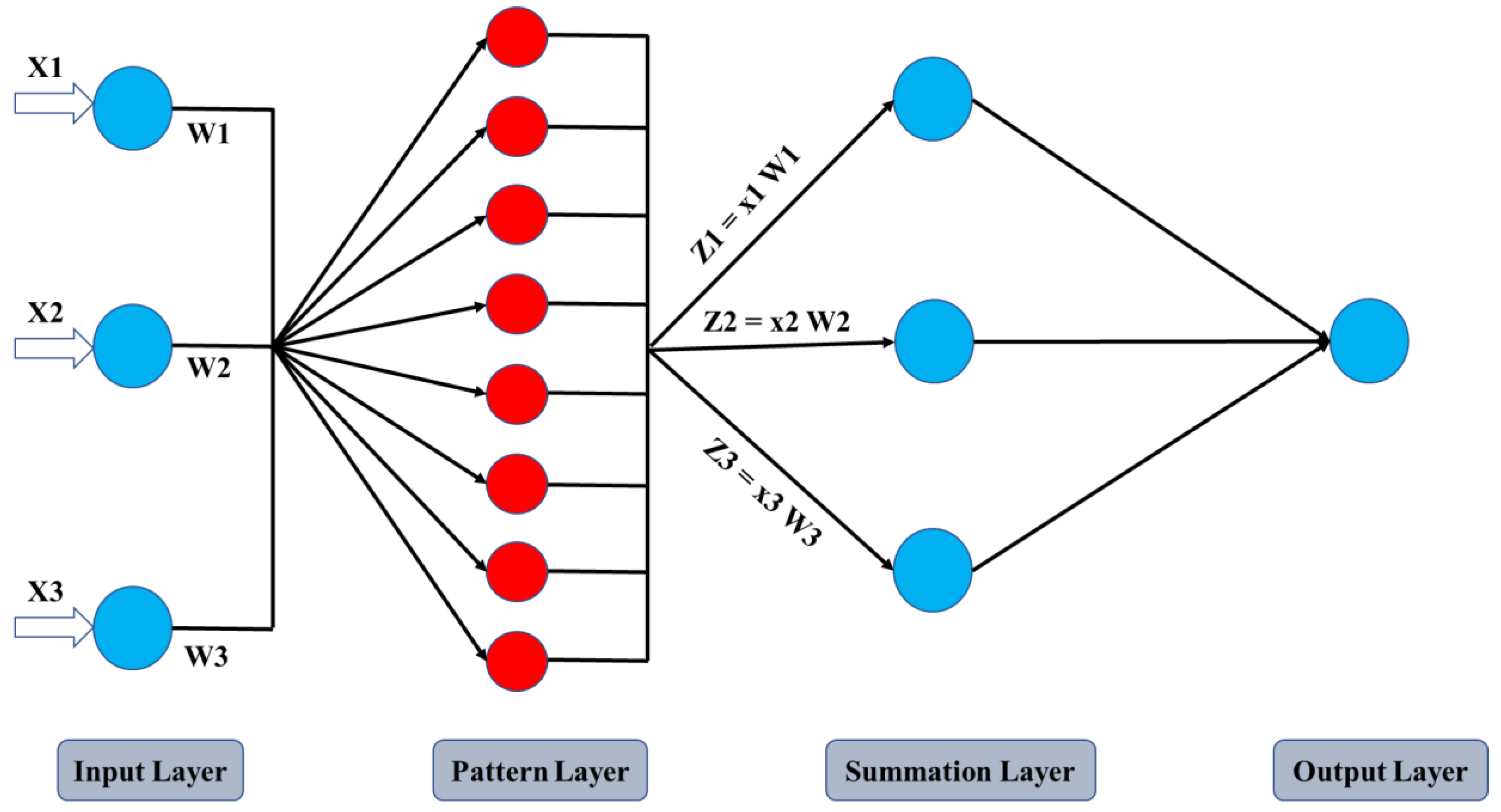
Although there is widespread use of AI in WQ modelling, there are currently a number of problems, including time-consuming algorithms, human modelling engagement, challenges in tuning internal parameters, and a lack of generality [35,36]. As a result, new and resilient mathematical models with significant flexibility in managing complex environmental issues are being developed [37]. The motivation of exploring new versions of AI models have always been the target of engineers and scientists. Recently, the probabilistic neural network has gained popularity for its capacity to effectively handle difficult regression problems [38,39,40,41,42]. Hence, this study was initiated to develop probabilistic neural network model in comparison with multi-layer perceptron ANN for the better estimation of BOD₅ and DO using the available WQ indicators, such as turbidity, temperature (T), pH- value, calcium (Ca), Sulfate (SO4), alkalinity, chemical oxygen demand (COD) total suspended solids (TSS), electrical conductivity (EC), and total dissolved solids (TDS). 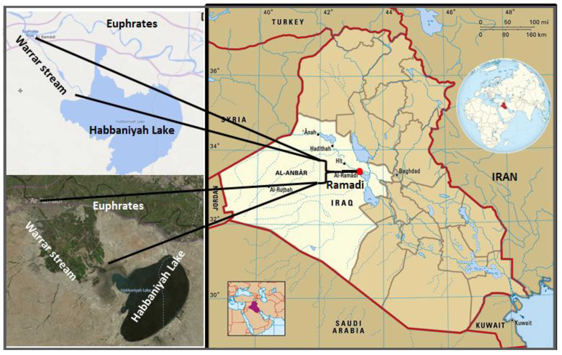This study was aimed at the development of a reliable mathematical formulation and model for good prediction of BOD₅ and DO in rivers for the improved management of water quality in areas where data availability is poor, such as Iraq. This is considered an important methodology for developing nations such as Iraq, where the funds allocated for environmental quality monitoring and evaluation are inadequate, yet water pollution is common and devastating. As a result, launching the present study is very important for developing an intelligent method to manage the water quality factors of Iraq’s streams and rivers.

2. Case Study and Methodological Overview

2.1. Case Study

Anbar Province is located in the semi-arid area of western Iraq. With an area of 138,579 km², it is the largest governorate in Iraq, constituting 32% (almost a third) of Iraq’s total area. The City of Ramadi is the center of Anbar Governorate and is situated at the intersection of the Euphrates River and Warrar stream, Warrar Stream linking the Habbaniyah Lake and Euphrates River. Habbaniyah Lake is located a short distance to the south of the city Ramadi. Habbaniyah lake water quality severs from pollution which, mostly due to discharge wastewater, there are many point sources on the Warrar canal [43,44]. The WQ characteristics of Warrar stream determined at Ramadi City, Anbar province, western Iraq (latitude 33°24′16.7″ N; longitude 43°17.5′2.4″ E) was taken in the research (Figure 1). Until now, many point sources discharge their waste into the stream without any treatment, such as agricultural drainage, sewage, or even dispose solid waste. Because of the weakness of the environmental management, the Warrar stream’s water quality has decreased and deteriorated over time. Additionally, Warrar stream flows into Habbaniyah lake, which will be impacted also. Therefore, the prediction of WQ of Warrar stream is very important for regional environmental quality monitoring and management. The wastewater samples at the end of the point sources discharges were collected, field and laboratory tests of water quality variables were carried out in the Anbar Directorate of Environment laboratories. The sampling frequency was collected monthly over the period of 2006–2015. The availability of long-term reliable WQ data is a main challenge in Iraq, as such data are only available for 10 years, and the supplied data were completely used in the current study. Sewage from residential areas and agricultural areas are the main sources of water pollution in the Warrar stream. The water quality of the Warrar stream is quite low. Furthermore, untreated wastewater discharge into the stream introduces a major risk of many forms of water pollutants. The physical and chemical factors such as turbidity, temperature, pH, Ca, SO4, TDS, alkalinity, and TSS were used as inputs to initiate the prediction models.

2.2. Methodology

• Multi-Layer Perceptron Neural Network Method (MLPNN)

MLP is a subcategory of FFNN. Neurons in MLP should be arranged in a one-directional pattern. In MLP, data is transitioned between three types of parallel layers: input, hidden, and output. Some weights contained inside [1, 1] should be used to characterize the links between the layers [45,46]. Summation and activation are two functions that each node in the MLP can perform [47,48]. The summing function in Equation (1) sums the product of inputs, weights, and bias.

$$S_j={\displaystyle \sum }_{i=1}^n{w}_{ij}{I}_i+{\beta }_i$$

(1)

$I_i$ is the input variable (i) while j is the bias term; $w_{ij}$ is the connection weight while n is the number of inputs. There are numerous sorts of activation functions available in the MLP. Previous research has mostly employed the S-shaped curved sigmoid function [49], Equation (2).

$$f_j\left(x\right)=\frac{1}{1+e^{-s_j}}$$

(2)

As a result, Equation (3) may be used to calculate the neuron j final output:

$$y_i=f_i\left({\displaystyle \sum }_{i=1}^n{w}_{ij}{I}_i+{\beta }_j\right)$$

(3)

The learning phase is used to fine-tune and update the weights of the network after creating the ANN’s structure. To reduce output error and estimate the outcomes, the network weights are rationalized. The training technique used by the NN is a demanding task that might reveal the MLP’s ability to address a variety of problems.

2.

Probabilistic Neural Network

Specht [50] proposed the probabilistic neural network (PNN) for the first time in 1989. It is a parallel approach that hybridized the Bayes categorization principles and the likelihood density formula estimate approach of the Parzen window. PNN is a supervised learning NN commonly used in fault detection and pattern recognition. The advantage of PNN in practical applications, particularly in fault detection, is that it applies a linear learning algorithm method to accomplish the work done by a nonlinear learning algorithm while maintaining the nonlinear method’s very high precision and other properties.

PNN is a feedforward NN that is established on the RBS network; it has the Bayesian minimum risk criteria called Bayesian decision theory as its theoretical foundation. PNN is a form of RBN mostly used in pattern detection. Figure 2 depicts the PNN’s basic construction. The input layer, pattern layer, summation layer, and output layer are the four layers that make up this system. The distribution of sample data is the corresponding weight of PNN, and the network is capable of meeting real-time data processing in training without the need for a training phase.

The feature vectors from the training samples are received by the input layer, which then sends them to PNN for processing. The size of the training sample feature vectors determines how many neurons are in the input layer. The feature vectors X are made up of each neuron and the wight vectors W where Z = XW is the input variables for the input layer. The relationship between each node and the input feature vector in the training data is determined by the pattern layer. The pattern layer has the same number of neurons as the sum of the training data for each defect class. Each mode unit in this layer has the following output:

$$f\left(X,W_i\right)=exp\left[-\frac{{(X-W_i)}^T\left(X-W_i\right)}{2{\delta }^2}\right]$$

(4)

where the smoothing factor is denoted as $W_i$, the input feature vectors are denoted as X, and the connection weight between the input and pattern layers is denoted by $W_i$.

The summarizing layer is the third layer; this layer combines the probabilities that belonged to a specific class previously and computes the probability amount based on the earlier described approach to get the probability density function (PDF) of the fault category. There is just one summation layer neuron in each of the fault categories, which is coupled with the mode layer neuron of the same fault category but not with those of others inside the mode layer. As a result, the sum layer neuron’s only purpose is to sum up the outputs of the pattern layer neurons that belong to its own fault category, without considering the outputs of neurons that belong to the other fault categories. The predicted probability density for each of the fault categories is comparable to the output of the summing layer’s neurons. To estimate the likelihood of each fault category, the output layer can be normalized as follows:

$$P(\frac{X}{W_i}=\frac{1}{{(2\pi )}^{\frac{n}{2}}{\delta }^n{N}_i}{\displaystyle \sum }_{j=1}^{N_i}exp\left[-\frac{{(X-W_i)}^T\left(X-W_i\right)}{2{\delta }^2}\right]$$

(5)

where X_ij is W_i’s column sample, n is the sample features vectors’ size, and N_i is W_i’s test sum.

The output layer of the PNN is comprised of a threshold discriminator that serves in the selection of the neuron with the best posterior PDF which will act as the system’s output from the probability density estimated for each of the defect kinds. The number of neurons in the output layer equates the number of different forms of training sample data received from the sum output layer of varying fault kinds. One of the largest PDFs of the neuron output is 1, which typifies the kind of fault category of the unknown samples, with values ranging from 0 to 1. The nearest classifier is utilized once the distribution density SPREAD value is approaching 0; however, when the SPREAD amount is high, it serves as an adjacent classifier for a given number of training examples.

3. Results

Water quality prediction models can be used to examine the trend of water quality degradation. As previously stated, the main focus of our research was on the simulation of two key chemical factors (i.e., BOD₅ and DO). Both metrics have been traditionally employed as indicators of water quality for decades, and good prediction is unquestionably necessary in this scenario to facilitate preventative measures. This paper presents a novel predictive PPNN model that was compared to the MLP for performance. PNN is a relatively new method that uses an approximation tool to anticipate complex patterns. The suggested model’s superiority is tested by examining several types of errors in model simulation. The prediction results were analyzed and evaluate using several standers such as correlation coefficient, mean absolute error (MAE), root mean square error (RMSE), mean bias error (MBE) and others [36].

Table 1. The characteristics of the water quality parameters that were measured.

Parameter	Unit	Min.	Max.	Average	SD	Median
Temperature	°C	9	38	21.8	8.07	22
Turbidity	NTU	8.6	72.6	20.4	15.5	13.2
pH	-	7.4	8	7.7	0.14	7.8
EC	μs/cm	1271	1858	1442	127.5	1402
Alkalinity	Mg/L	99	158	121	12.5	120
Ca	Mg/L	84	119	96.2	8.25	94
Mg	Mg/L	42	95	66.2	11.8	68
SO4	Mg/L	241	511	427	36.7	429
T.D.S	Mg/L	845	1253	1069	91.4	1079
T.S.S	Mg/L	11	188	55.4	47.9	34.5
Na	Mg/L	108	183	135.6	14.3	136
BOD5	Mg/L	2.72	5.28	3.94	0.58	3.85
COD	Mg/L	9.13	118.8	12.7	9.9	11.5
DO	Mg/L	5.52	7.96	6.83	0.61	6.88

reveals the results of an exploratory analysis of the WQ factors of the Euphrates River. The correlations of each input parameter with BOD and DO were calculated to help understand the impact of each predictor on the specified variables (

Table 2. The correlation magnitude between each WQ variable and BOD₅ and DO.

Input Variables	BOD5	DO
Temperature	0.47	0.61
pH	0.34	0.36
Turbidity	0.32	0.38
EC	0.28	0.29
Ca	0.13	0.12
Alkalinity	0.31	0.37
COD	0.26	0.28
SO4	0.08	0.05
TSS	0.19	0.21
TDS	0.22	0.25

). Except for temperature, all the water quality metrics had low and negligible correlation coefficients. The BOD and DO were predicted using a total of eight parameters. In this regard, four separate models were built using a mix of different input parameters and labeled (M1, M2, …, M4).

Model 1 (M1), as seen in

Table 3. The input combinations to estimate DO and BOD₅ WQ variables.

Models	Input Combinations
Model-1	$\mathrm{M}1=\mathrm{Temperature} \left(\mathrm{T}\right)$
Model-2	$\mathrm{M}2=\mathrm{Temperature} \left(\mathrm{T}\right), \mathrm{pH}$
Model-3	$\mathrm{M}3=\mathrm{Temperature} \left(\mathrm{T}\right), \mathrm{Turbidity}, \mathrm{pH}$
Model-4	$\mathrm{M}4=\mathrm{Temperature} \left(\mathrm{T}\right), \mathrm{Turbidity}, \mathrm{pH}, \mathrm{Alkalinity}$

, has only temperature as its WQ parameter, while M2 and M4 have two and four WQ parameters as input attributes. Increases in the number of parameters (from 1 to 4 for M1 to M4) improved the performance of the model by revealing the relevance of each of the included parameters. To further understand the level sensitivity of the 5 input WQ variables used in this research to predict DO and BOD₅, four models were built in the current research.

3.1. Dissolved Oxygen Prediction

Table 4. Statistical indicators values using MLPNN method during testing period.

Model	RMSE	MAE	MBE	NSE	SI	BIAS	d	CI
Model-1	0.440	0.360	0.020	0.996	0.064	−0.120	0.996	0.992
Model-2	0.254	0.194	0.012	0.999	0.037	−0.072	0.999	0.997
Model-3	0.389	0.312	−0.011	0.997	0.057	0.093	0.997	0.994
Model-4	0.270	0.223	−0.002	0.998	0.039	0.024	0.999	0.997

and

Table 5. Statistical indicators values using PNN method during testing period.

Model	RMSE	MAE	MBE	NSE	SI	BIAS	d	CI
Model-1	0.306	0.240	−0.010	0.998	0.045	0.075	0.998	0.996
Model-2	0.222	0.175	−0.014	0.999	0.032	0.098	0.999	0.999
Model-3	0.177	0.146	−0.009	0.999	0.026	0.063	0.999	0.998
Model-4	0.245	0.205	0.001	0.999	0.036	0.005	0.999	0.997

show the predictive accuracy of MLPNN and PPNN, respectively. The PNN was shown to perform exceptionally well in the simulation of DO utilizing the third input combination (M3), based on the supplied values (temperature, turbidity, and pH). The standard approach (MLPNN), on the other hand, achieved the greatest results for the second input combination (M2) for DO prediction. This is attributed mainly to the fact that the mathematical models react differently depending on the specificity of the underlying mechanism between both the predictor and the predictand in each scenario.

The scatter plots in Figure 3 and Figure 4 show the effectiveness of the algorithm in predicting DO. The best DO prediction results were obtained by PNN method using a third model. Whereas MLPNN achieved a good prediction whiling utilizing the second input combination. The PNN prediction model performed better than the top MLPNN model. PNN yielded the strongest correlation R², 0.94 (Model-3), whereas MLPNN yielded 0.84 (Model-2).

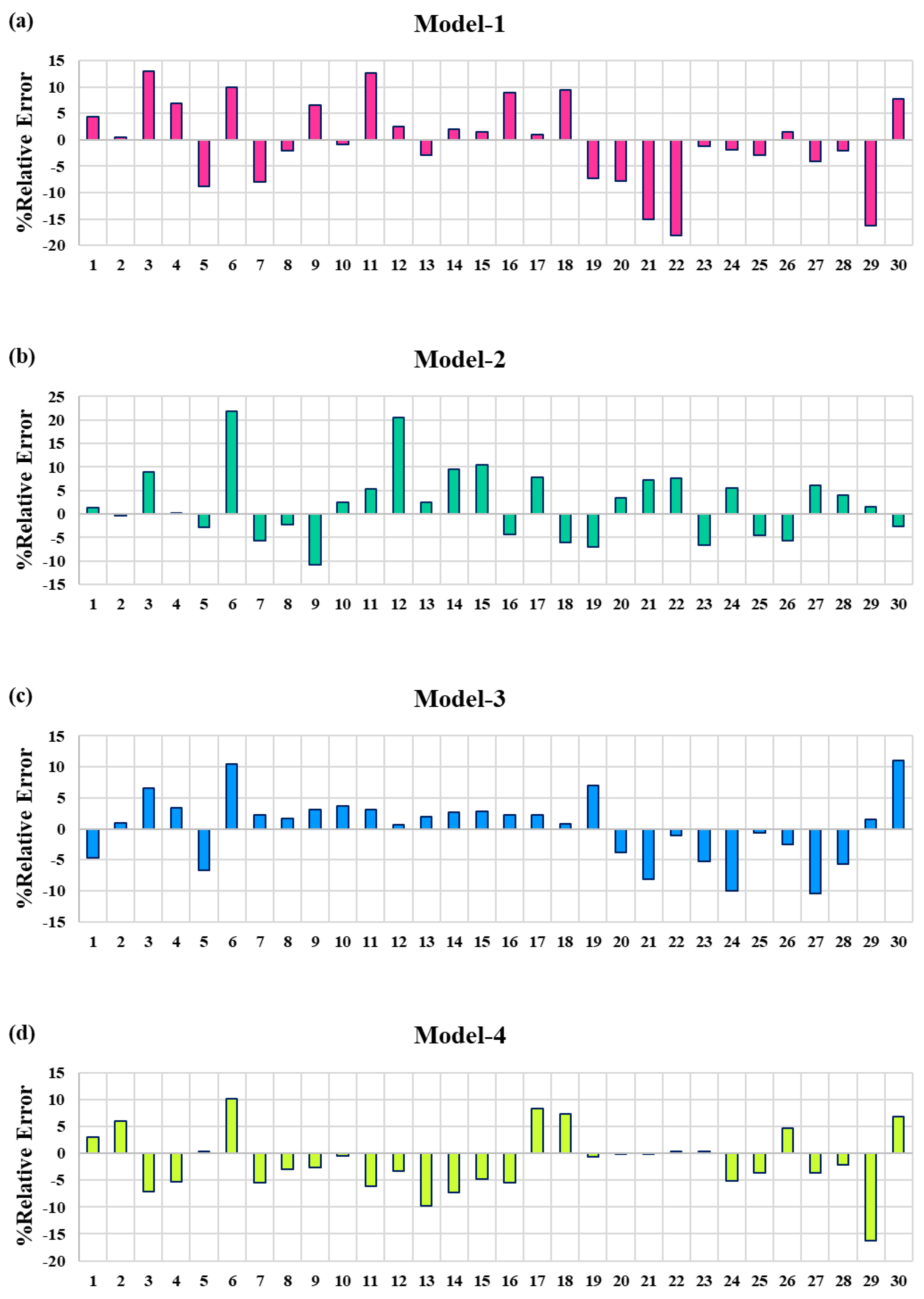
In order to provide clearer assessment of the effectiveness of the suggested methods, the outcomes of the best input combinations are illuminated utilizing more sensitive indicators. Figure 5 and Figure 6 show the percentage relative error for each model over the testing period. In all situations, the predictive results revealed that the PNN had much less error than the MLPNN. For example, the greatest percentage error for MLPNN with the fourth model is +10%, whereas the PNN achieved a percentage error of less than +7% with the same input combination. According to the relative error indicator, it is clear that PNN resulted in a significant improvement in the prediction results. Similarly, other assessment indicators revealed very encouraging results employing PNN for DO prediction.

3.2. Biochemical Oxygen Demand Prediction

The performance of the proposed methods for DOD prediction was evaluated based on several statistical indicators, as presented in

Table 6. Statistical indicators values using MLPNN method during testing period.

Model	RMSE	MAE	MBE	NSE	SI	BIAS	d	CI
Model-1	0.322	0.255	−0.004	0.994	0.076	0.026	0.995	0.989
Model-2	0.212	0.174	0.003	0.997	0.050	−0.003	0.995	0.992
Model-3	0.318	0.256	0.022	0.994	0.075	−0.083	0.998	0.992
Model-4	0.246	0.195	−0.015	0.987	0.058	0.068	0.997	0.993

and

Table 7. Statistical indicators values using PNN method during testing period.

Model	RMSE	MAE	MBE	NSE	SI	BIAS	d	CI
Model-1	0.317	0.262	0.031	0.994	0.074	−0.129	0.995	0.989
Model-2	0.145	0.116	−0.008	0.999	0.034	0.036	0.999	0.998
Model-3	0.231	0.197	−0.012	0.997	0.054	0.053	0.997	0.994
Model-4	0.230	0.175	−0.017	0.997	0.054	0.075	0.997	0.994

. The results revealed that both models (i.e., MLPNN and PNN) provide acceptable prediction accuracy when trained with two different parameters (Model-2). This finding is consistent with the significant correlation results in Table 2, which show temperature and pH as the key factors influencing BOD values. In fact, the fundamental objective of the predictor method should be to attain better results for prediction rather than adding more input variables in the process. From the standpoint of laboratory efforts, it is quite crucial. This is also extremely useful for catchments where there are limited or scare environmental data. The results suggest the need to focus on WQ variables that have high significant effects on the internal relationships and prediction process, as the addition of more WQ parameters to a model could sometimes confuse it, leading to erroneous predictions or leading it astray.

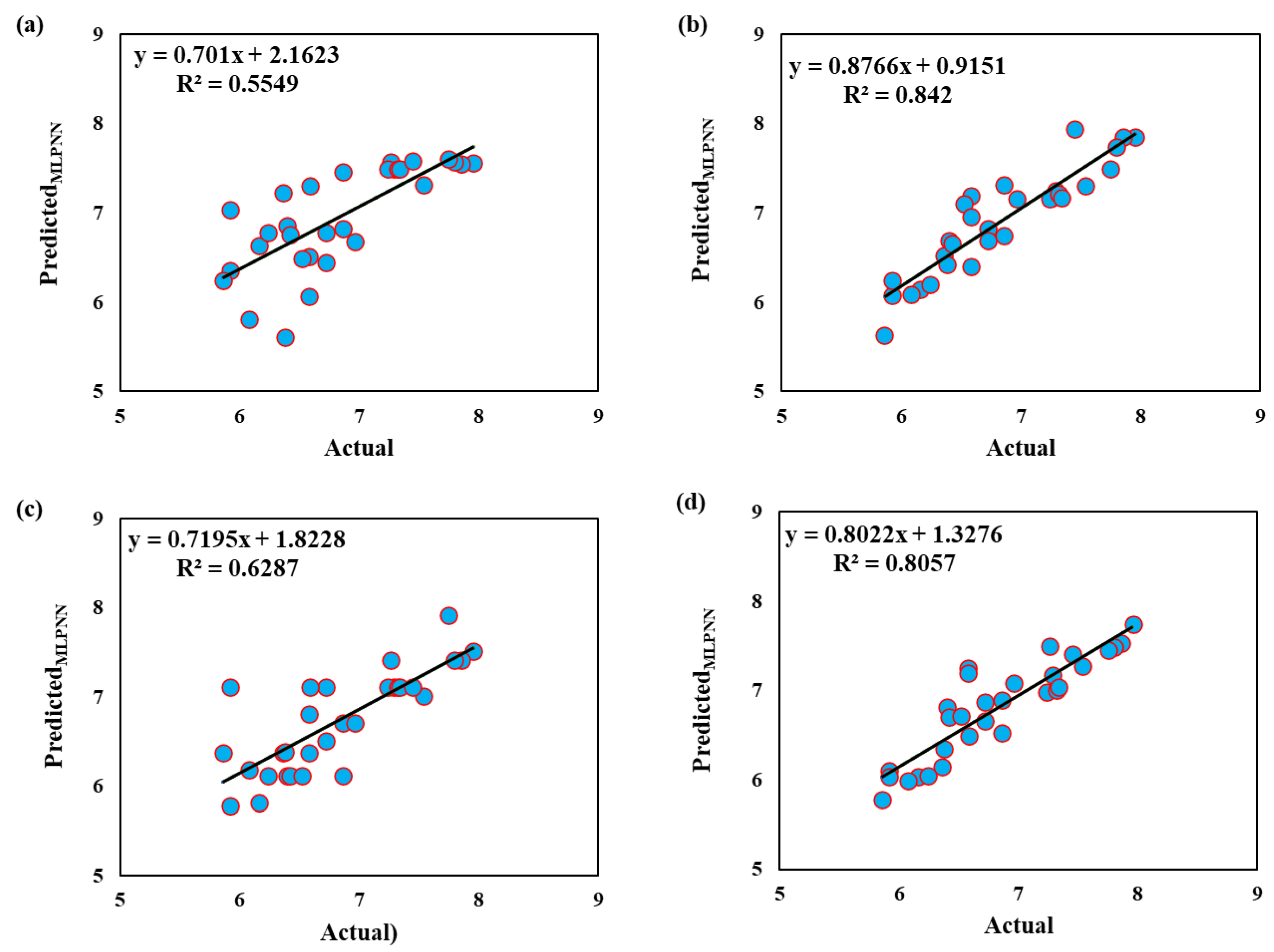
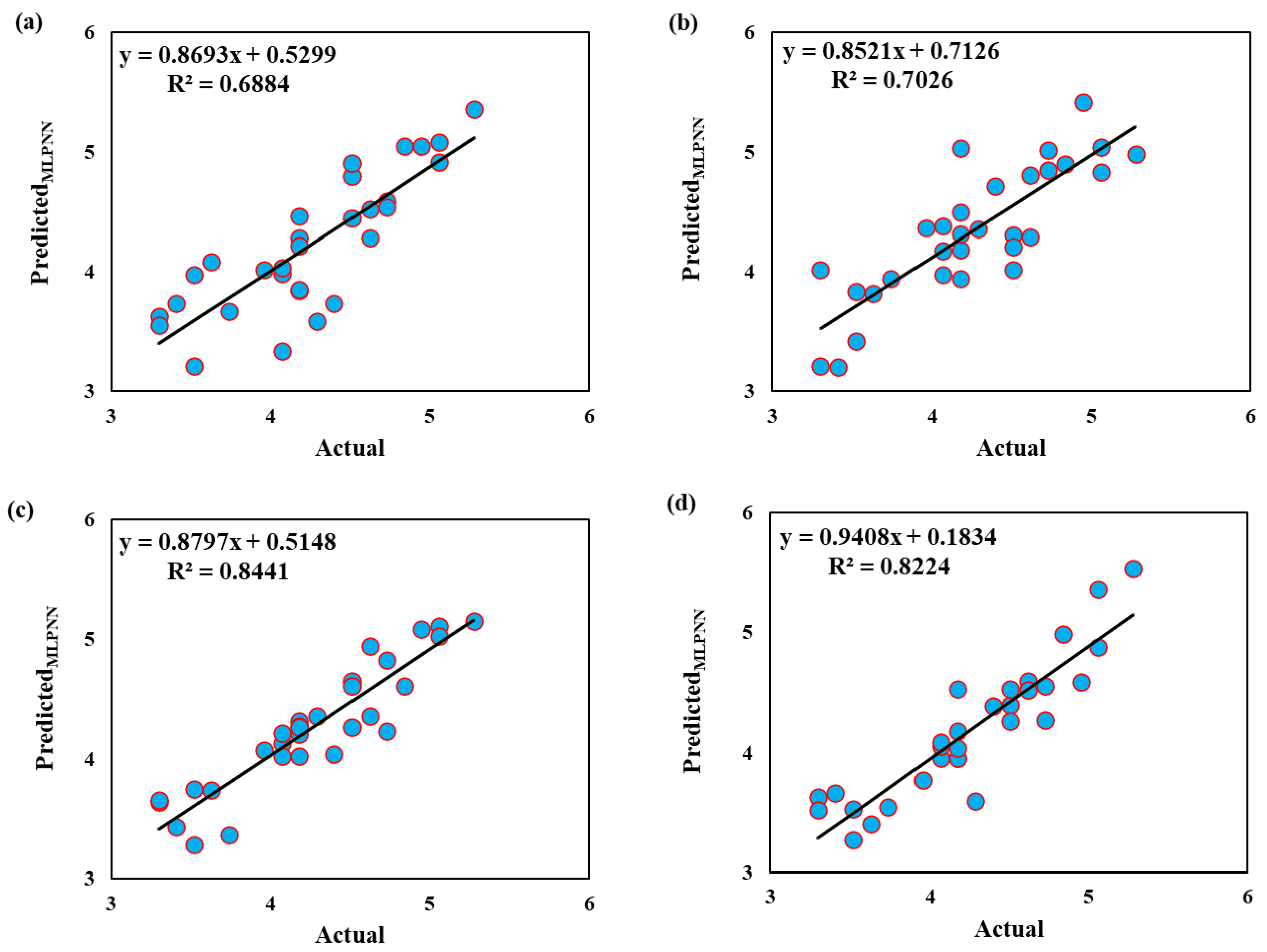
Figure 7 shows the performance of the MLPNN model during the testing stage utilizing scatter plots. The BOD prediction for all proposed models (M1:M4) are presented. The MLPNN model achieved better accuracy with the third and fourth input combinations. The lowest reliability was attained with the first input combination. MLPNN yielded the strongest correlation (0.84) with Model-3. The visualization of the diversion from the identical line clearly is presented more closely and this clearly presenting the matching between the actual observations and the predicted values.

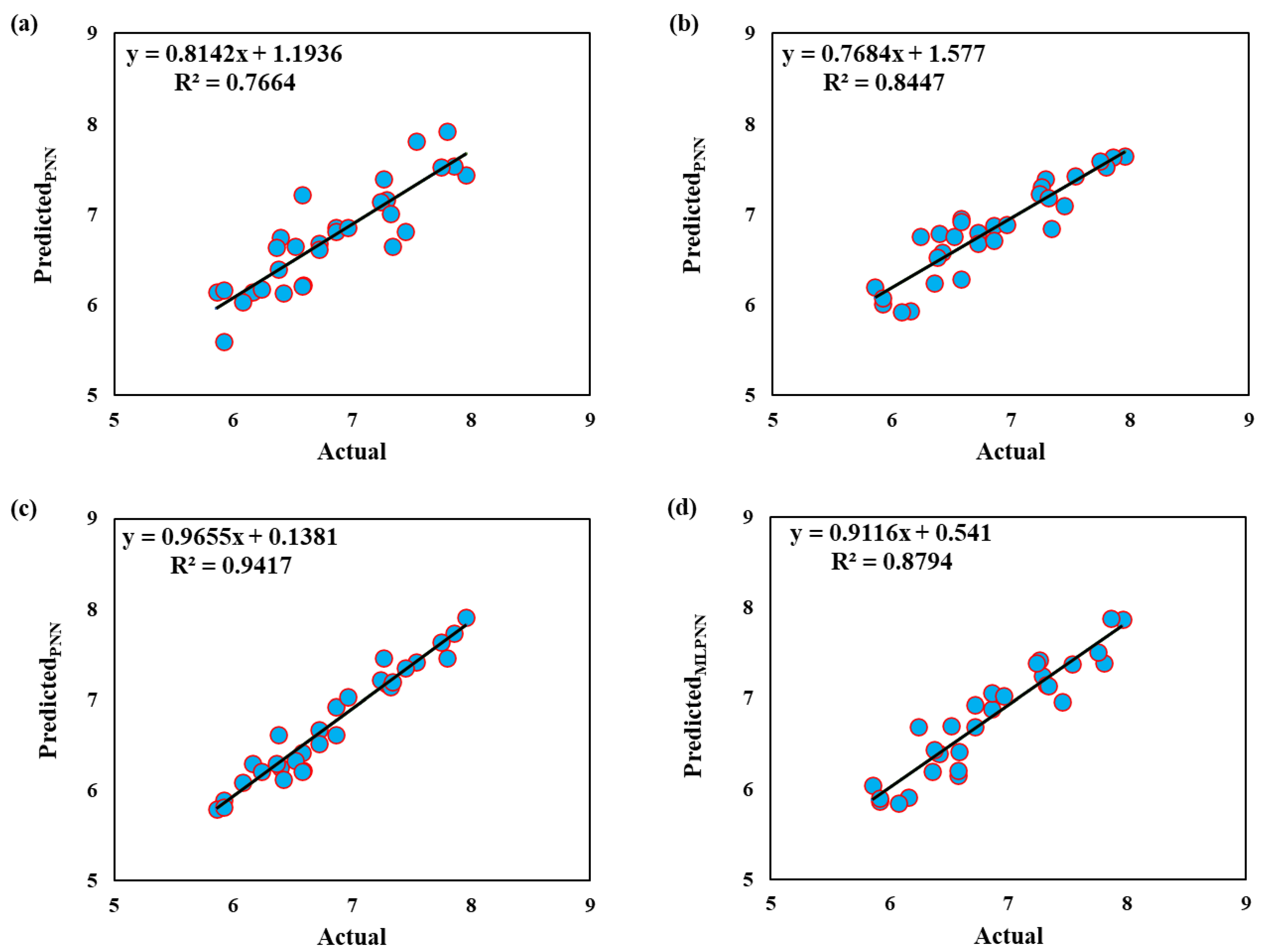
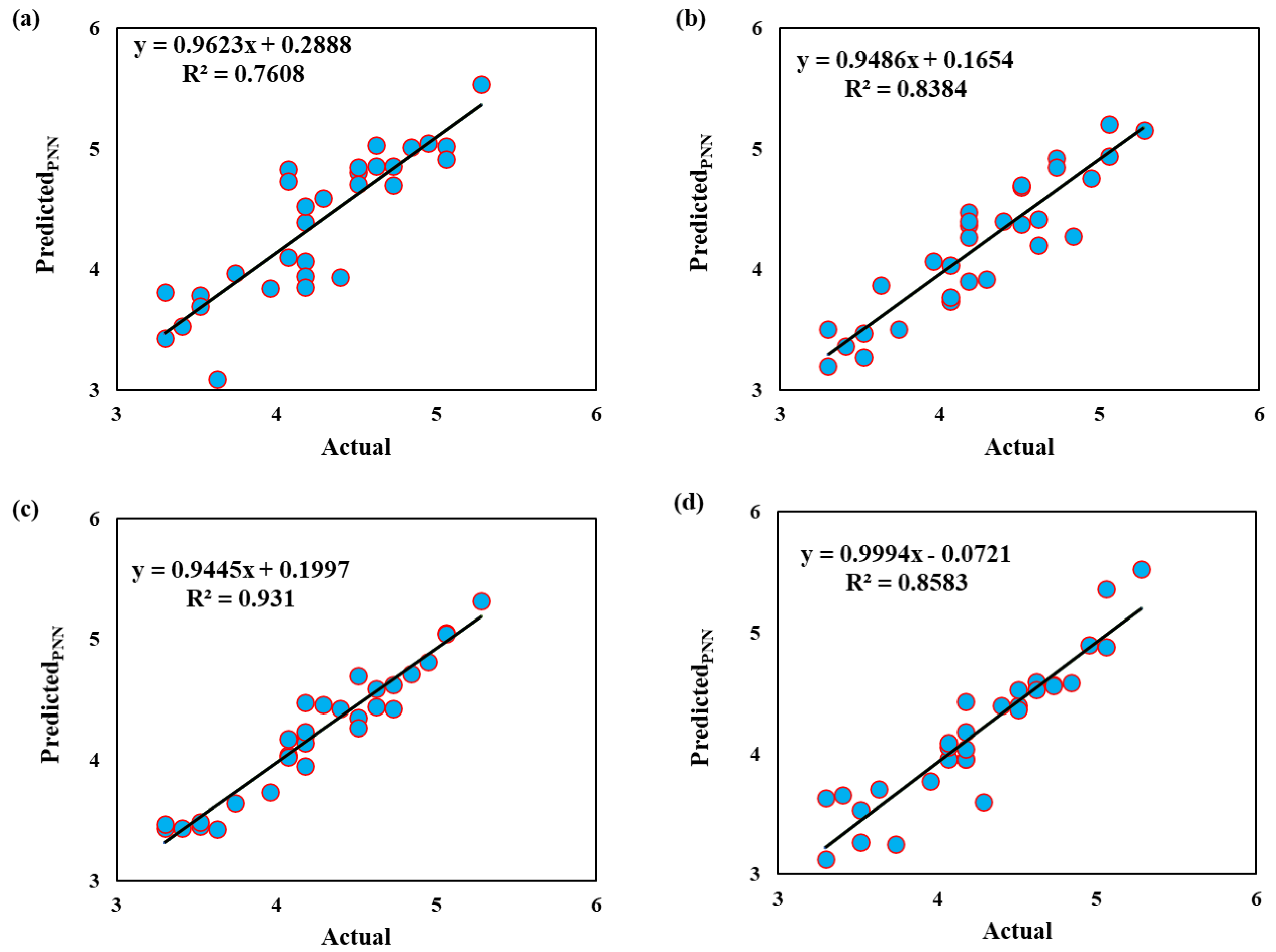
The scatter plots for all proposed input combinations employing PNN method are exhibited in Figure 8. In general, the PNN succeeded in providing acceptable prediction results. The correlation magnitude between actual and predicted data for all models is presented. It could be noted that the PNN attained high correlation with third input combinations, (R² = 0.93). The results revealed that the PNN is superior to the MLPNN method in predicting the BOD variable according to the correlation coefficient indicator. For this modeling scenario, near perfection of scattering was attained between the actual observations and the predicted values.

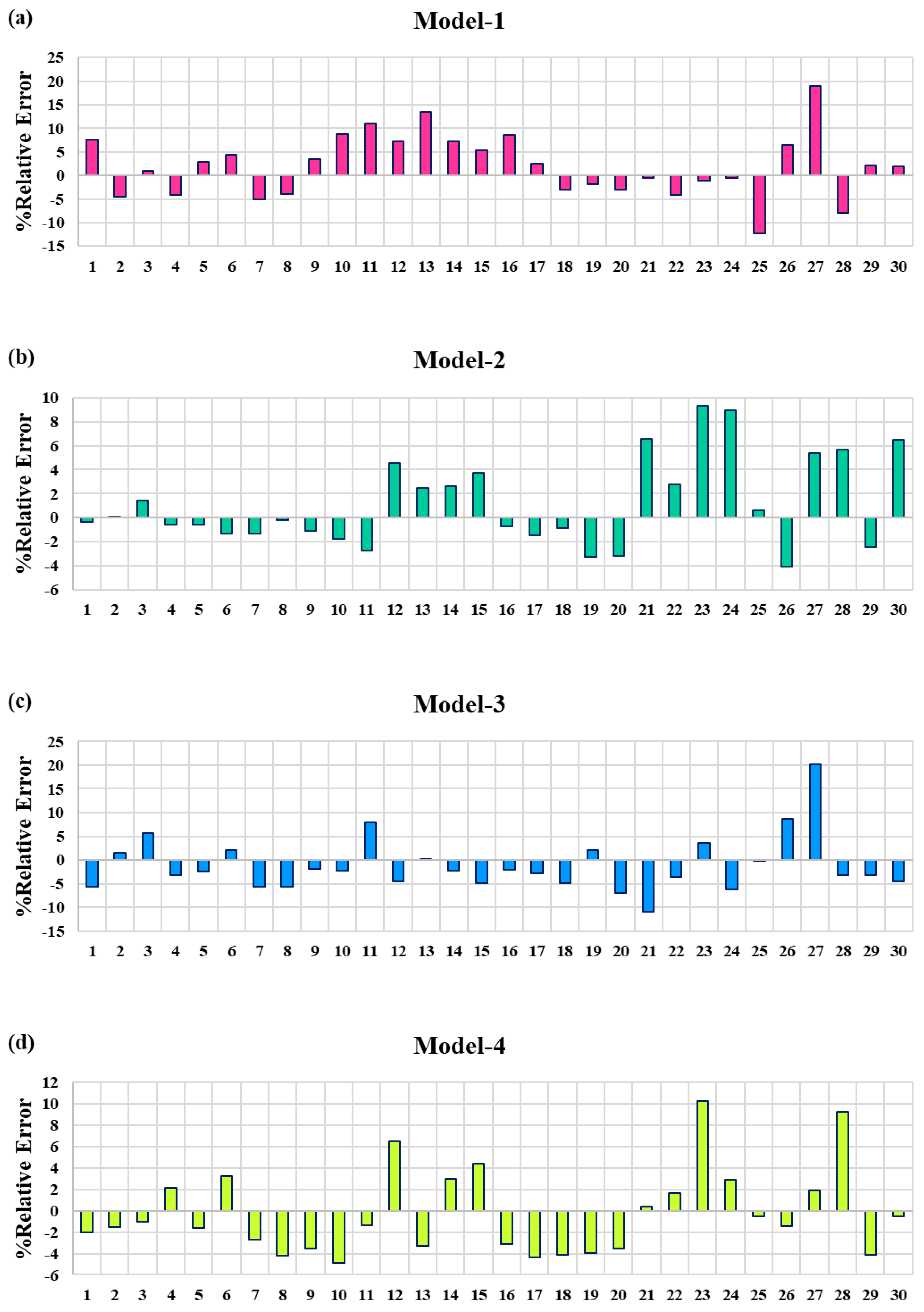
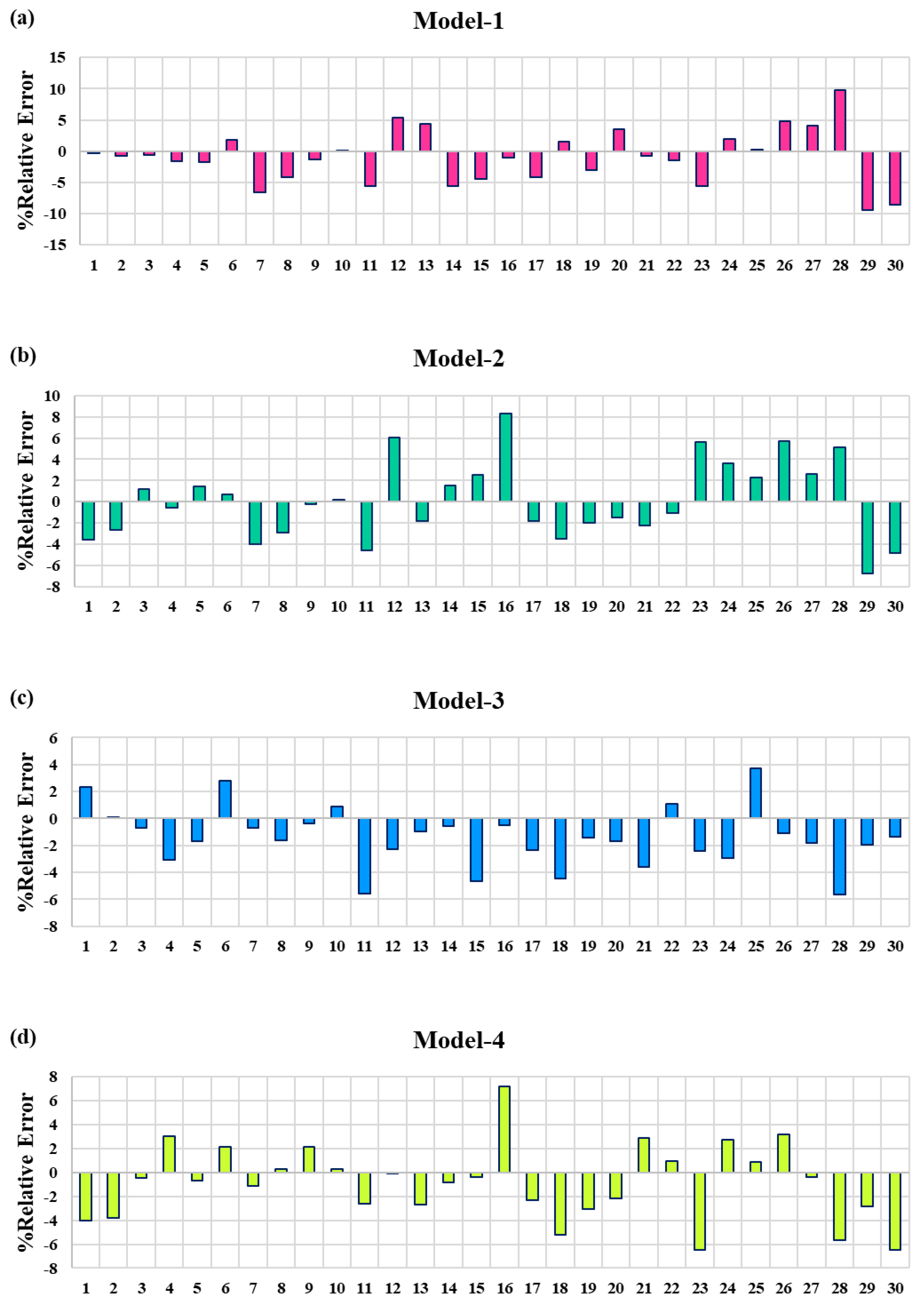
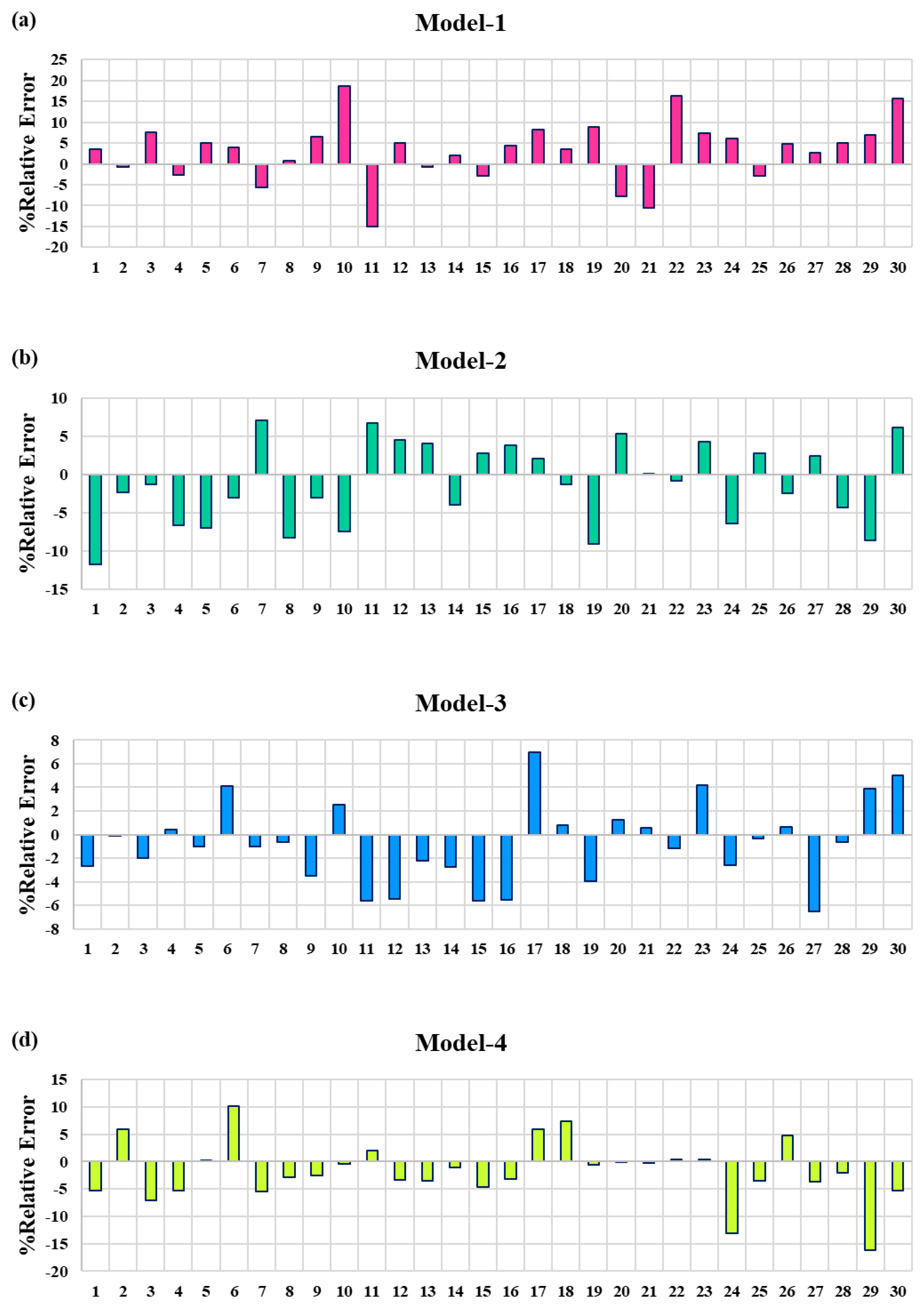
The distribution of the percentage relative error for all the proposed models utilizing both prediction methods (i.e., MLPNN and PNN) are shown in Figure 9 and Figure 10. It is observed that the minimum error is achieved by depending on third input combination for MLPNN and PNN methods. By comparing the proposed methods, the performance of PNN was superior to that of MLPNN, and the maximum error was +7%.

The evaluation indicators showed that both methods provided acceptable accuracy for the prediction of WQ factors. By highlighting PNN, it is a method capable of assigning a multidimensional pattern of outcome variable responses to changes in control variables that influence the system’s physical processes. The technique’s strength rests in its ability to capture accurate smooth approximations of responses by using a collection of polynomial functions that can capture the nonlinearity in system behavior. The capacity to use high-order polynomial functions for precise approximation of responses is PNN’s key advantage over other AI techniques. As a result, it has greater explanatory power than previous AI-based regression analyses. Polynomial-based approximations are smooth, which eliminates numeric fluctuation and allows for accurate response variable prediction. Through basic measurements of river water temperature, turbidity and pH, the models created in the current research can be used to forecast BOD and DO at every place along the Euphrates River. It is commonly known that DO has an inverse relationship with temperature and turbidity in a river, whereas BOD has a direct relationship with temperature and turbidity. The prediction method (i.e., PNN) with the most appropriate input combinations succussed for providing better accuracy compared to MLPNN method.

4. Conclusions

The feasibility of a modern method, PNN, in predicting water quality variables was investigated in this study. The PNN was used to predict BOD₅ and DO parameters in water of Euphrates River. The goal of developing this method was to create a reliable tool for determining environmental quality parameters based on past laboratory data. As input attributes, the models were created utilizing several physical and chemical WQ factors of water. The models were built using laboratory data collected over a period between January 2006 to December 2015. The performance of the PNN method was compared to the MLPNN model, which is a well-known predictive framework. The prediction accuracy obtained by PNN was higher compared with the MLPNN method. The optimal evaluation indicators for PNN in predicting BOD are (R² = 0.93, RMSE = 0.231 and MAE = 0.197). The best performance indicators for PNN in predicting Do are (R² = 0.94, RMSE = 0.222 and MAE = 0.175).

Furthermore, both suggested models showed less reasonable approximation values in terms of the input attributes, which is critical for BOD₅ and DO prediction in river system with limited environmental, aqueous, or ecological data. Overall, the findings showed that PNN may be utilized to forecast water quality characteristics in the Euphrates River. Future studies should focus on incorporating additional useful input features, such as hydrological, bacteriological or even climatological factors to maximize the precision of prediction models. Furthermore, the viability of natural-inspired algorithms for selecting appropriate casual information between predictors and predictands can be investigated.

References

1. Tiyasha, T.; Tung, T.M.; Yaseen, Z.M. Deep Learning for Prediction of Water Quality Index Classification: Tropical Catchment Environmental Assessment. Nat. Resour. Res. 2021, 30, 4235–4254. [Google Scholar] [CrossRef]
2. Gleick, P.H. Global freshwater resources: Soft-path solutions for the 21st century. Science 2003, 302, 1524–1528. [Google Scholar] [CrossRef] [PubMed] [Green Version]
3. Du Plessis, A. Persistent degradation: Global water quality challenges and required actions. One Earth 2022, 5, 129–131. [Google Scholar] [CrossRef]
4. Yaseen, Z.M.; Ramal, M.M.; Diop, L.; Jaafar, O.; Demir, V.; Kisi, O. Hybrid Adaptive Neuro-Fuzzy Models for Water Quality Index Estimation. Water Resour. Manag. 2018, 32, 2227–2245. [Google Scholar] [CrossRef]
5. Yaseen, Z.M.; Ehteram, M.; Sharafati, A.; Shahid, S.; Al-Ansari, N.; El-Shafie, A. The Integration of Nature-Inspired Algorithms with Least Square Support Vector Regression Models: Application to Modeling River Dissolved Oxygen Concentration. Water 2018, 10, 1124. [Google Scholar] [CrossRef] [Green Version]
6. Najafzadeh, M.; Homaei, F.; Farhadi, H. Reliability assessment of water quality index based on guidelines of national sanitation foundation in natural streams: Integration of remote sensing and data-driven models. Artif. Intell. Rev. 2021, 54, 4619–4651. [Google Scholar] [CrossRef]
7. Ighalo, J.O.; Adeniyi, A.G.; Marques, G. Artificial intelligence for surface water quality monitoring and assessment: A systematic literature analysis. Model. Earth Syst. Environ. 2021, 7, 669–681. [Google Scholar] [CrossRef]
8. Armanuos, A.; Ahmed, K.; Shiru, M.S.; Jamei, M. Impact of Increasing Pumping Discharge on Groundwater Level in the Nile Delta Aquifer, Egypt. Knowl.-Based Eng. Sci. 2021, 2, 13–23. [Google Scholar] [CrossRef]
9. Kareem, S.L.; Jaber, W.S.; Al-Maliki, L.A.; Al-husseiny, R.A.; Al-Mamoori, S.K.; Alansari, N. Water quality assessment and phosphorus effect using water quality indices: Euphrates River-Iraq as a case study. Groundw. Sustain. Dev. 2021, 14, 100630. [Google Scholar] [CrossRef]
10. Oleiwi, S.; Jalal, S.; Hamed, S.; Ozgur, S.; Zaher, K.; Yaseen, M. Precipitation pattern modeling using cross-station perception: Regional investigation. Environ. Earth Sci. 2018, 77, 709. [Google Scholar]
11. Ahmed, A.N.; Othman, F.B.; Afan, H.A.; Ibrahim, R.K.; Fai, C.M.; Hossain, M.S.; Ehteram, M.; Elshafie, A. Machine learning methods for better water quality prediction. J. Hydrol. 2019, 578, 124084. [Google Scholar] [CrossRef]
12. Kerachian, R.; Karamouz, M. A stochastic conflict resolution model for water quality management in reservoir—River systems. Adv. Water Resour. 2007, 30, 866–882. [Google Scholar] [CrossRef]
13. Zhi, W.; Feng, D.; Tsai, W.-P.; Sterle, G.; Harpold, A.; Shen, C.; Li, L. From hydrometeorology to river water quality: Can a deep learning model predict dissolved oxygen at the continental scale? Environ. Sci. Technol. 2021, 55, 2357–2368. [Google Scholar] [CrossRef]
14. Fitri, A.; Maulud, K.N.A.; Rossi, F.; Dewantoro, F.; Harsanto, P.; Zuhairi, N.Z. Spatial and Temporal Distribution of Dissolved Oxygen and Suspended Sediment in Kelantan River Basin. In Proceedings of the 4th International Conference on Sustainable Innovation 2020—Technology, Engineering and Agriculture (ICoSITEA 2020), Yogyakarta, Indonesia, 13–14 October 2020; Atlantis Press: Dordrecht, The Netherlands, 2021; pp. 51–54. [Google Scholar]
15. Tao, H.; Bobaker, A.M.; Ramal, M.M.; Yaseen, Z.M.; Hossain, M.S.; Shahid, S. Determination of biochemical oxygen demand and dissolved oxygen for semi-arid river environment: Application of soft computing models. Environ. Sci. Pollut. Res. 2019, 26, 923–937. [Google Scholar] [CrossRef] [PubMed]
16. Tiyasha; Tung, T.M.; Yaseen, Z.M. A survey on river water quality modelling using artificial intelligence models: 2000–2020. J. Hydrol. 2020, 585, 124670. [Google Scholar] [CrossRef]
17. Moreno-Guerrero, A.-J.; López-Belmonte, J.; Marín-Marín, J.-A.; Soler-Costa, R. Scientific development of educational artificial intelligence in Web of Science. Future Internet 2020, 12, 124. [Google Scholar] [CrossRef]
18. Naganna, S.R.; Beyaztas, B.H.; Bokde, N.; Armanuos, A.M. On the Evaluation of the Gradient Tree Boosting Model for Groundwater Level Forecasting. Knowl.-Based Eng. Sci. 2020, 1, 48–57. [Google Scholar] [CrossRef]
19. Jamei, M.; Ahmadianfar, I.; Karbasi, M.; Jawad, A.H.; Farooque, A.A.; Yaseen, Z.M. The assessment of emerging data-intelligence technologies for modeling Mg+2 and SO4−2 surface water quality. J. Environ. Manag. 2021, 300, 113774. [Google Scholar] [CrossRef]
20. Shiri, N.; Shiri, J.; Yaseen, Z.M.; Kim, S.; Chung, I.M.; Nourani, V.; Zounemat-Kermani, M. Development of artificial intelligence models for well groundwater quality simulation: Different modeling scenarios. PLoS ONE 2021, 16, e0251510. [Google Scholar] [CrossRef]
21. Bhagat, S.K.; Tiyasha, T.; Kumar, A.; Malik, T.; Jawad, A.H.; Khedher, K.M.; Deo, R.C.; Yaseen, Z.M. Integrative artificial intelligence models for Australian coastal sediment lead prediction: An investigation of in-situ measurements and meteorological parameters effects. J. Environ. Manag. 2022, 309, 114711. [Google Scholar] [CrossRef]
22. Ahmadianfar, I.; Shirvani-Hosseini, S.; He, J.; Samadi-Koucheksaraee, A.; Yaseen, Z.M. An improved adaptive neuro fuzzy inference system model using conjoined metaheuristic algorithms for electrical conductivity prediction. Sci. Rep. 2022, 12, 4934. [Google Scholar] [CrossRef] [PubMed]
23. Malik, A.; Saggi, M.K.; Rehman, S.; Sajjad, H.; Inyurt, S.; Bhatia, A.S.; Farooque, A.A.; Oudah, A.Y.; Yaseen, Z.M. Deep learning versus gradient boosting machine for pan evaporation prediction. Eng. Appl. Comput. Fluid Mech. 2022, 16, 570–587. [Google Scholar] [CrossRef]
24. Jamei, M.; Karbasi, M.; Alawi, O.A.; Kamar, H.M.; Khedher, K.M.; Abba, S.I.; Yaseen, Z.M. Earth skin temperature long-term prediction using novel extended Kalman filter integrated with Artificial Intelligence models and information gain feature selection. Sustain. Comput. Inform. Syst. 2022, 35, 100721. [Google Scholar] [CrossRef]
25. Tur, R.; Yontem, S. A Comparison of Soft Computing Methods for the Prediction of Wave Height Parameters. Knowl.-Based Eng. Sci. 2021, 2, 31–46. [Google Scholar] [CrossRef]
26. Barzegar, R.; Adamowski, J.; Moghaddam, A.A. Application of wavelet-artificial intelligence hybrid models for water quality prediction: A case study in Aji-Chay River, Iran. Stoch. Environ. Res. Risk Assess. 2016, 30, 1797–1819. [Google Scholar] [CrossRef]
27. Maier, H.R.; Dandy, G.C. The use of artificial neural networks for the prediction of water quality parameters. Water Resour. Res. 1996, 32, 1013–1022. [Google Scholar] [CrossRef]
28. Hameed, M.; Sharqi, S.S.; Yaseen, Z.M.; Afan, H.A.; Hussain, A.; Elshafie, A. Application of artificial intelligence (AI) techniques in water quality index prediction: A case study in tropical region, Malaysia. Neural Comput. Appl. 2017, 28, 893–905. [Google Scholar] [CrossRef]
29. Azad, A.; Karami, H.; Farzin, S.; Saeedian, A.; Kashi, H.; Sayyahi, F. Prediction of water quality parameters using ANFIS optimized by intelligence algorithms (case study: Gorganrood River). KSCE J. Civ. Eng. 2018, 22, 2206–2213. [Google Scholar] [CrossRef]
30. Tiwari, S.; Babbar, R.; Kaur, G. Performance Evaluation of Two ANFIS Models for Predicting Water Quality Index of River Satluj (India). Adv. Civ. Eng. 2018, 2018, 8971079. [Google Scholar] [CrossRef] [Green Version]
31. Xiang, Y.; Jiang, L. Water Quality Prediction Using LS-SVM and Particle Swarm Optimization. In Proceedings of the 2009 Second International Workshop on Knowledge Discovery and Data Mining, Moscow, Russia, 23–25 January 2009; pp. 900–904. [Google Scholar]
32. Haghiabi, A.H.; Nasrolahi, A.H.; Parsaie, A. Water quality prediction using machine learning methods. Water Qual. Res. J. Can. 2018, 53, 3–13. [Google Scholar] [CrossRef]
33. Jamei, M.; Ahmadianfar, I.; Chu, X.; Yaseen, Z.M. Prediction of surface water total dissolved solids using hybridized wavelet-multigene genetic programming: New approach. J. Hydrol. 2020, 589, 125335. [Google Scholar] [CrossRef]
34. Aryafar, A.; Khosravi, V.; Zarepourfard, H.; Rooki, R. Evolving genetic programming and other AI-based models for estimating groundwater quality parameters of the Khezri plain, Eastern Iran. Environ. Earth Sci. 2019, 78, 69. [Google Scholar] [CrossRef]
35. Danandeh Mehr, A.; Rikhtehgar Ghiasi, A.; Yaseen, Z.M.; Sorman, A.U.; Abualigah, L. A novel intelligent deep learning predictive model for meteorological drought forecasting. J. Ambient. Intell. Humaniz. Comput. 2022, 1–15. [Google Scholar] [CrossRef]
36. Yaseen, Z.M. An insight into machine learning models era in simulating soil, water bodies and adsorption heavy metals: Review, challenges and solutions. Chemosphere 2021, 277, 130126. [Google Scholar] [CrossRef] [PubMed]
37. Behmel, S.; Damour, M.; Ludwig, R.; Rodriguez, M.J. Water quality monitoring strategies—A review and future perspectives. Sci. Total Environ. 2016, 571, 1312–1329. [Google Scholar] [CrossRef] [PubMed]
38. Cho, S.J.; Hermsmeier, M.A. Genetic algorithm guided selection: Variable selection and subset selection. J. Chem. Inf. Comput. Sci. 2002, 42, 927–936. [Google Scholar] [CrossRef] [PubMed]
39. Wei, D.; Cui, Z.; Chen, J. Optimization and tolerance prediction of sheet metal forming process using response surface model. Comput. Mater. Sci. 2008, 42, 228–233. [Google Scholar] [CrossRef]
40. Kewlani, G.; Iagnemma, K. A stochastic response surface approach to statistical prediction of mobile robot mobility. In Proceedings of the 2008 IEEE/RSJ International Conference on Intelligent Robots and Systems, IROS, Nice, France, 22–26 September 2008. [Google Scholar]
41. Acherjee, B.; Misra, D.; Bose, D.; Venkadeshwaran, K. Prediction of weld strength and seam width for laser transmission welding of thermoplastic using response surface methodology. Opt. Laser Technol. 2009, 41, 956–967. [Google Scholar] [CrossRef]
42. Roussouly, N.; Petitjean, F.; Salaun, M. A new adaptive response surface method for reliability analysis. Probabilistic Eng. Mech. 2013, 32, 103–115. [Google Scholar] [CrossRef] [Green Version]
43. Ghalib, H.S.; Ramal, M.M. Spatial and temporal water quality evaluation of heavy metals of Habbaniyah Lake, Iraq. Int. J. Des. Nat. Ecodyn. 2021, 16, 467–475. [Google Scholar] [CrossRef]
44. Khaleefa, O.; Kamel, A.H. On The Evaluation of Water Quality Index: Case Study of Euphrates River, Iraq. Knowl.-Based Eng. Sci. 2021, 2, 35–43. [Google Scholar] [CrossRef]
45. Allawi, M.F.; Jaafar, O.; Mohamad Hamzah, F.; Ehteram, M.; Hossain, M.S.; El-Shafie, A. Operating a reservoir system based on the shark machine learning algorithm. Environ. Earth Sci. 2018, 77, 366. [Google Scholar] [CrossRef]
46. Osman, A.; Afan, H.A.; Allawi, M.F.; Jaafar, O.; Noureldin, A.; Hamzah, F.M.; Ahmed, A.N.; El-Shafie, A. Adaptive Fast Orthogonal Search (FOS) algorithm for forecasting streamflow. J. Hydrol. 2020, 586, 124896. [Google Scholar] [CrossRef]
47. Allawi, M.F.; Aidan, I.A.; El-Shafie, A. Enhancing the performance of data-driven models for monthly reservoir evaporation prediction. Environ. Sci. Pollut. Res. 2021, 28, 8281–8295. [Google Scholar] [CrossRef] [PubMed]
48. Allawi, M.F.; Ahmed, M.L.; Aidan, I.A.; Deo, R.C.; El-Shafie, A. Developing reservoir evaporation predictive model for successful dam management. Stoch. Environ. Res. Risk Assess. 2021, 35, 499–514. [Google Scholar] [CrossRef]
49. Kashiwao, T.; Nakayama, K.; Ando, S.; Ikeda, K.; Lee, M.; Bahadori, A. A neural network-based local rainfall prediction system using meteorological data on the Internet: A case study using data from the Japan Meteorological Agency. Appl. Soft Comput. J. 2017, 56, 317–330. [Google Scholar] [CrossRef]
50. Specht, D.F. Probabilistic neural networks. Neural Netw. 1990, 3, 109–118. [Google Scholar] [CrossRef]
Figure 1. The case study location of Warrar stream in Iraq.
Mathematics 10 03960 g001
Figure 2. Probabilistic Neural Network Architecture.
Mathematics 10 03960 g002
Figure 3. Scatter Plots for the MLNN method: (a) Model-1; (b) Model-2; (c) Model-3; and (d) Model-4, respectively.
Mathematics 10 03960 g003
Figure 4. Scatter Plots for the PNN method: (a) Model-1; (b) Model-2; (c) Model-3; and (d) Model-4, respectively.
Mathematics 10 03960 g004
Figure 5. Distribution of the relative error through examination interval for all models using MLPNN method.
Mathematics 10 03960 g005
Figure 6. Distribution of the relative error through examination interval for all models using PNN method.
Mathematics 10 03960 g006
Figure 7. Scatter Plots for the MLPNN method: (a) Model-1; (b) Model-2; (c) Model-3; and (d) Model-4, respectively.
Mathematics 10 03960 g007
Figure 8. Scatter Plots for the PNN method: (a) Model-1; (b) Model-2; (c) Model-3; and (d) Model-4, respectively.
Mathematics 10 03960 g008
Figure 9. Distribution of the relative error through examination interval for all models using MLPNN method.
Mathematics 10 03960 g009
Figure 10. Distribution of the relative error through examination interval for all models using PNN method.
Mathematics 10 03960 g010