Article

Age-Dependent Survival Rates in SIR-SI Dengue Transmission Model and Its Application Considering Human Vaccination and Wolbachia Infection in Mosquitoes

1
Department of Mathematics, Faculty of Mathematics and Natural Sciences, Universitas Padjadjaran, Sumedang 45363, Indonesia
2
Department of Industrial Engineering, Faculty of Engineering, Universitas Langlangbuana, Bandung 40261, Indonesia
3
Center for Mathematical Modeling and Simulation, Institut Technologi Bandung, Jl. Ganesha 10, Bandung 40132, Indonesia
4
Differential Equations, Modeling, and Simulation Group, Department of Mathematics, Indian Institute of Technology Indore, Indore 453552, India
5
Humanities Research Group, Institut Technologi Bandung, Jl. Ganesha 10, Bandung 40132, Indonesia
6
International Program of Science Education, Universitas Pendidikan Indonesia, Jl. Dr. Setiabudhi 229, Bandung 40154, Indonesia
*
Author to whom correspondence should be addressed.
Mathematics 2022, 10(21), 3950; https://doi.org/10.3390/math10213950
Submission received: 29 August 2022 / Revised: 18 October 2022 / Accepted: 20 October 2022 / Published: 24 October 2022
(This article belongs to the Section Mathematical Biology)

Abstract

:
In this paper, an SIR-SI mathematical model in the form of a system of integral equations describing the transmission of dengue disease between human and mosquitoes is proposed and analyzed. Age-dependent functions are used to describe the survival of individuals in human and mosquito populations. The basic reproduction number is derived and its relationship to the equilibria is also explored. The results show that the existence of the positive endemic equilibrium is determined by a threshold number. This threshold number is also the same one that determines the global stability of the equilibrium. The threshold acts like the known basic reproduction number in the counterpart differential equations model and also follows the same rule for the critical level of intervention. Furthermore, as an application, the effect of wolbachia infection is explored, such as how this infection changes the resulting threshold and what the consequence of its presence is in the dynamics of the disease. In this case, the decrease of the mosquitoes’ life expectancy and biting rate are used to reflect the effect of wolbachia bacterial infection on the mosquitoes. In other words, a mosquito which is infected by wolbachia has a lower life expectancy than a normal mosquito. The results, both from mathematical analysis and numerical examples, show that the presence of wolbachia has the potential as a biological control agent to eliminate the dengue in the human population. A comparison of the wolbachia introduction into the mosquito population with the existing strategy, such as vaccination, is also presented.

1. Introduction

Vector-borne infectious diseases are among the serious health problems faced by many tropical countries. An example is the dengue disease, which is transmitted by mosquitoes that may lead to fatality in some cases. Four identified strains of flavivirus, namely DEN-1, DEN-2, DEN-3, and DEN-4, are responsible for the disease. Although it is reported that some mosquitoes, such as Aedes albopictus, are able to transmit the disease, but the main vector which is responsible for the transmission is the female of Aedes aegypti. Due to frequent, large outbreaks of the disease in many countries, some attempts are continuously undertaken to eliminate the disease, such as fogging the adult-class of the mosquitoes using an insecticide and introducing predators to the larvae-class of the mosquitoes [1,2]. Beside those attempts, several efforts, such as developing a safe vaccine that can protect humans from all known strains of dengue viruses are being developed, and some other means have already become available as common practices [3,4].
Mathematical models have been known among the tools to understand the phenomena of the transmission of infectious diseases for a long time [5,6]. Many studies have been devoted to dengue dynamic modeling [7,8,9,10]. Various complexities considering many important factors, such as physiological- and age-structures, have been added to existing models to increase the realism of the models. Many scientists believe that these are important factors that should be included in population dynamic modeling in general [11,12,13,14,15,16]. The authors in [17] have shown the contribution of age structure in some important biological processes, such as therapeutic consequences in a disease cure. The theory of age structure in the general population model is well presented in a seminal book [18]. In disease dynamic modeling with direct transmission or with non-transmitted disease, examples that incorporate age structure in the models are abundant [19,20,21,22,23]. However, although many mathematical models have been devoted to address issues in dengue disease transmission, most of the authors have ignored age structure, with few exceptions, such as [24,25,26]. Some authors have studied age structure less explicitly, for example, by only looking at the effects of age on a certain population parameter, such as survival rates [19,27].
In this paper we discuss an SIR dengue transmission model with age-dependent survival rates by generalizing the model in [19] to include host-vector interactions, assuming that the survival rate of individuals varies as their age goes up by following a certain function. Here we assume that the function is monotonically non-increasing with respect to age. The underlying model is closely related to the works in [28,29], but here we perform a more rigorous and complete analysis. The former work [28] applied the model without examining the mathematical properties of the model, while the latter [29] discussed some preliminary properties of the model. The existence of a solution to a system of equations and its stability to a small perturbation is vital in providing a sound recommendation to confine the spread of disease represented by the system of those equations. The works in [28,29] have claimed the existence and stability of the non-trivial solution for a certain threshold value without giving the proof of it analytically. In this paper, we show the proof of the existence of the trivial and non-trivial solutions of the model and discuss the stability properties of the solutions. We also show that there is an endemic threshold in which the disease disappears whenever the threshold value is below one and the disease will stay endemic whenever the threshold value is above one. Furthermore, it will be shown that the critical level of vaccination rule generalizes to the age-structured host-vector transmission model. This work is regarded as necessary to support the application discussed in [28], where otherwise the validity of the recommendation based on the model therein is questionable.
Following [28], the model is then applied to assess the presence of the wolbachia infected mosquito population to control the natural mosquito population. Recently, many scientists have pointed out that an introduction of bacteria from the genus wolbachia into the vector mosquitoes may reduce the transmission of dengue disease [30,31]. Wolbachia infection reduces the biting rate of the dengue fever mosquito, Aedes aegypti, by destroying the mosquito’s proboscis so that it is difficult to penetrate human skin. The infection also reduces the life span of the mosquitoes [32]. It is reported that the use of wolbachia infection in mosquitoes seems prospective in controlling dengue disease. However, a study regarding its effect compared to other control strategies, such as doing nothing and vaccination, from different analogous/counterpart models is still needed to show the robustness of this kind of attempt in controlling dengue disease. This paper aims to fill this gap via mathematical modeling by first developing a different kind of dengue transmission model, i.e., by constructing a system of integral equations, followed by its application in comparing the transmission between the cases of absence and presence of wolbachia in the system. In this model (in the presence of a wolbachia infected population) we assume that the mosquito’s life expectancy and biting rate decrease due to the presence of wolbachia bacterial infection in the mosquito population.

2. Materials and Methods

Brauer in [19] discussed a mathematical model for an epidemic of S and I compartments in which he assumed a permanent infection in the form of a system of integral equations. Later on, this model was generalized into an SIR case in [29]. The model is closely related to the SIR model in [33]. Like the authors in [19,29], the authors in [33] consider generational recruitment as one of the vital dynamics in their model. However, other complexities, such as the dependency of survival on age, are not considered in [33] but are taken into account in [19,29]. In [19,29], the authors assume a direct transmission of infection occurs to a susceptible individual from an infective individual. In the present paper we generalize their models to include vector-born transmitted disease by assuming indirect transmission of the disease, such as in dengue disease transmission, in which human infection is caused by infective mosquitoes (not an infective human). We also include recovery in the model; hence the disease is not permanent.
To formulate the model, we assume that the host population N H is divided into three compartments, namely susceptibles S H , infectives I H , and recovered individuals R H ,   and hence N H = S H + I H + R H .   We assume that recovered host individuals are immune to the disease. However, we assume that infective vectors remain infective for life. This is because the duration of the disease is relatively long compared to the short life period of the mosquitoes. Hence, the vector population only has two compartments, namely susceptibles S V and infectives I V ,   to form N V = S V + I V . Recruitment rates for the host and the vector are B H and B V , with death rates μ H and μ V , respectively. The disease transmission probability from vector to host and from host to vector are given by β H and β V , respectively. Furthermore, it is assumed that there exist the functions Q H a and Q V a   which describe the fractions of the host and vector populations that survive to the age of a or more. These functions are non-negative monotonically decreasing with respect to age, satisfying Q H 0 = 1 and Q V 0 = 1 . These functions are introduced to mimic the age structure effect on the survival rates. The functions are closely related to the probability of being alive at time t0 + t, provided an individual is alive at time t0 as suggested by [33]. The difference is that in this paper we use a decreasing function with respect to age, while in [33] the authors assume a decreasing function independent of age (see Section 4 as an example).
Here we assume that the life expectancy of the host is finite,
0 Q H a d a = L H ,
so that
0 a Q H a d a < .
Furthermore,
N H t = 0 B H Q H a d a = B H L H .
The notations X a = B H Q H a and Y a = B V Q V a will be used to indicate the portion of offspring that survive to the age a or more. The number of susceptibles at time t is given by
S H t = S ˜ H t + 0 t X a E a , t , I V d a ,
with S ˜ H t = S H 0 Q H t e 0 t β H I V s d s and E a , t , I V = e t a t β H I V s d s , since B H I V t is the per capita rate of infection in the host population at time t . Here, e t a t β H I V s d s is the fraction of susceptibles of the age t a that survive to time t or more and are still free from dengue. Furthermore, the number of infective hosts at time t is given by
I H t = I ˜ H t + 0 t X a 1 E a , t , I V e γ a d a ,
if we assume that the rate of recovery is given by γ , with I ˜ H t = I H 0 Q H t e γ t . Here 1 E a , t , I V e γ a is the fraction of the infective host of the age t a that are alive at least up until time t and still have not recovered yet. Furthermore, since R H t = N H t S H t I H t , then we have
R H t = R ˜ H t + 0 t X a E a , t , I V ¯ 1 e γ a d a ,
with R ˜ H t = N ˜ H t S ˜ H t I ˜ H t and E a , t , I V ¯ 1 e γ a as the fraction of the recovered host of the age t a that survive at least up to time t . Note that, throughout the paper, we simplify some notations using an over line symbol which is defined similarly to the symbol that was just described for the E a , t , I V ¯ notation. Note that the transmission dynamics in the host population are given by Equations (4)–(6).
Similarly, since
N V t = N ˜ V t + 0 t Y a d a = B V L V ,
with L V = 0 Q V a d a , the transmission dynamics in the vector population are given by
S V t = S ˜ V t + 0 t Y a F a , t , I H d a ,
with S ˜ V t = S V 0 Q V t e 0 t β V I H s d s , and F a , t , I H = e t a t β V I H s d s , and
I V t = I ˜ V t + 0 t Y a 1 F a , t , I H d a ,
with I ˜ V = I V 0 Q V t . Hence, Equations (4)–(6), (8) and (9) govern the complete model for the SIR-SI host-vector dengue transmission model. In the next section we analyze these equations and look for the equilibria of the model. We also look for a threshold epidemic R 0 which determines the existence of the non-trivial equilibrium. In the subsequent section we also show that the stability of the non-trivial equilibrium point is indeed determined by this threshold.

3. Results

3.1. The Boundedness of the Solution

The boundedness of the solution for the human compartment is readily given from the fact that for all t we have N H t = S H t + I H t + R H t = B H L H < , so that S H t < ,   I H t < , and R H t <   for all t . Analogously, we also have the boundedness of the solution for the vector compartment, i.e., S V t <   and I V t <   for all t .

3.2. The Positivity of the Solution

First, let us see the solutions for the human compartment. It is clear from (3) that for all t we have N H t = B H L H > 0 . Considering I V t <   for all t , then we have the number of susceptibles from (4), S H t = S ˜ H t + 0 t X a E a , t , I V d a > 0 , since S ˜ H t = S H 0 Q H t e 0 t β H I V s d s > 0 and E a , t , I V = e t a t β H I V s d s > 0 . The number of infectives is given by (5) to be I H t = I ˜ H t + 0 t X a 1 E a , t , I V e γ a d a > 0 , since we have also E a , t , I V = e t a t β H I V s d s < 1 . Moreover, from (6), the recovery number is R H t = R ˜ H t + 0 t X a 1 E a , t , I V   1 e γ a d a > 0 , since E a , t , I V < 1 and e γ a < 1 . This proves that S H t > 0 ,   I H t > 0 , and R H t > 0 for all t . Finally, the positivity of the solutions for the vector compartment, i.e., S V t > 0 and I V t > 0   for all t , can be similarly proven.

3.3. The Existence of a Non-Trivial (Endemic) Equilibrium Point

In the epidemic modeling literature, the existence of a non-trivial or endemic equilibrium point is very important. This existence depends critically on a threshold number, which is often called the basic reproduction number [34,35]. In this section, we will formulate the basic reproduction number for the model discussed here. The basic reproduction number ( R 0 ) is defined as “the expected number of secondary cases produced, in a completely susceptible population, by a typical infective individual” [34]. In general, it can determine the stability of the non-endemic and endemic equilibria, in the sense that if R 0 < 1 then the non-endemic equilibrium is asymptotically stable, but unstable otherwise. Moreover, if R 0 > 1 then the endemic equilibrium is asymptotically stable [36] In our model, we also show that when R 0 > 1 , then the non-trivial equilibrium point is unique.
Since we are interested in the long-term behavior of the model, let us consider the limiting condition of (3) to (9), as in [19]. It is clear that lim t N ˜ V t = lim t S ˜ V t = lim t I ˜ V t = 0 since Q H a is a decreasing function. Hence, whenever t , the system consisting of these equations has the same behavior as the system of equations
S H t = 0 X a E a , t , I V d a ,
I H t = 0 X a 1 E a , t , I V e γ a d a ,
R H t = 0 X a E a , t , I V ¯ 1 e γ a d a ,
S V t = 0 Y a F a , t , I H d a ,
I V t = 0 Y a 1 F a , t , I H d a .
Here, we have (10) to (14) as a representation of the dynamics of an SIR-SI age-structured host-vector model.
The equilibria of the system, if they exist, are given by S H * ,   I H * ,   R H * ,   S V * ,   I V * with I H * and I V * satisfying
I H * = 0 X a 1 e β H a I V * e γ a d a = F 1 I V * ,
I V * = 0 Y a 1 e β V a I H * d a = F 2 I H *
Note that (15) can be written as I H * = F 1 F 2 I H * = F 1 F 2 I H * with
I H * = 0 X a 1 E ^ a , I H * e γ a d a ,
and E ^ a , I H * = e β H a [ 0 B V Q V s [ 1 e β V s I H * d s   . It is easy to see that N H * ,   0 ,   0 ,   N V * ,   0 is a trivial or disease-free equilibrium. To find a non-trivial endemic equilibrium, we could observe that F 1 F 2 is bounded and
d F 1 ( F 2 I H )   d I H > 0   and   d 2 F 1 ( F 2 I H )   d I H 2 < 0 .
This means that the function F 1 F 2 ( I H ) is concave downward. In order for the equation F 1 F 2   I H = I H to have a solution, we need d F 1 ( F 2 0 )   d I H > 1 . By considering this condition, together with the differentiation of Equation (17) with respect to I H it will result in d F 1 ( F 2 0 )   d I H = [ B H β H 0 a Q H a e γ a d a ]   [ B V β V 0 a Q V a d a ] > 1 . Next, by letting R 0 H = B H β H 0 a Q H a e γ a d a and R 0 V = B V β V 0 a Q V a d a , a unique non-trivial value of I H * exists whenever
R 0 = R 0 H R 0 V
is greater than 1. The existence of the corresponding non-trivial value of I V * follows immediately. The left-hand side of (19) is called the threshold number or the basic reproduction number of dengue transmission. We conclude that an endemic equilibrium S H * ,   I H * ,   R H * ,   S V * ,   I V * with I H * > 0 and I V * > 0 occurs whenever R 0 > 1 .

3.4. The Stability of the Equilibria

To investigate the stability of the equilibria, we use the method in [19] and the Gronwall-like inequality lemma therein.
Lemma 1
[19].Let  f t be a bounded non-negative continuous function satisfying
f t f 0 t + 0 t f t a R a d a ,  
where f 0 t is a non-negative continuous function with lim t f 0 t = 0 and R a is a non-negative continuous function with 0 R a d a < 1 . Then lim t f t = 0 .
It is also shown in [19] that the lemma is still true if the inequality in the lemma is replaced by
f t f 0 t + 0 t sup t a s t f s R a d a .
Further, we generalize Lemma 1 as follows.
Lemma 2.
Let f j t , j = 1 ,   2 be bounded non-negative continuous functions satisfying
f 1 t f 10 t + 0 t sup t a s t f 2 s R 1 a d a ,
f 2 t f 20 t + 0 t sup t a s t f 1 s R 2 a d a ,
where f j 0 t is non-negative continuous with lim t f j 0 t = 0 and R j a is non-negative continuous with 0 R j a d a < 1 . Then lim t f j t = 0 ,   j = 1 ,   2 .
Proof. 
A direct proof is given in [37]. The following is an alternative proof as a consequence of Lemma 1.
f 1 t sup f 10 t ,   f 20 t + 0 t sup t a s t sup f 1 s , f 2 s sup R 1 a , R 2 a d a , f 2 t sup f 10 t ,   f 20 t + 0 t sup t a s t sup f 1 s , f 2 s sup R 1 a , R 2 a d a ,
and hence
sup f 1 t , f 2 t sup f 10 t , f 20 t + 0 t sup t a s t S f S R d a ,
with S f = sup f 1 s , f 2 s and S R = sup R 1 a , R 2 a . Lemma 1 gives lim t sup f 1 s , f 2 s = 0 , and this is sufficient to conclude that lim t f j t = 0 ,   j = 1 ,   2 . □

3.4.1. The Stability of the Trivial (Disease-Free) Equilibrium

To investigate the stability of the equilibrium we will assume that R 0 < 1 . Consider the equilibrium infective class I H * , I V * = 0 , 0 and the following inequalities
1 e t a t β H I V s d s t a t β H I V s d s a β H sup t a s t I V s ,
1 e t a t β V I H s d s t a t β V I H s d s a β V sup t a s t I H s .
Hence, from (5) and (9) we have
I H t = I ˜ H t + 0 t X a 1 E a , t , I V e γ a d a I ˜ H t + 0 t X a [ a β H   sup t a s t I V s ] e γ a d a ,
I V t = I ˜ V t + 0 t Y a 1 F a , t , I H d a I ˜ V t + 0 t Y a [ a β V   sup t a s t I H s ] d a ,
If we further assume that 0 a β H X a e γ a d a < 1 and 0 a β V Y a d a < 1 , then using Lemma 2 we conclude that lim t I H t = 0 and lim t I V t = 0 . This shows that the disease-free (trivial) equilibrium is globally stable irrespective of the initial values I H 0 and I V 0 .

3.4.2. The Stability of the Non-Trivial (Endemic) Equilibrium

The endemic equilibrium, i.e., S H * , I H * , R H * , S V * , I V * with I H * > 0 and I V * > 0 , occurs if and only if R 0 > 1 . Let us see the perturbations of I H * and I V * , respectively, by v t and u t . Define I H t = I H * + v t and I V t = I V * + u t , and substitute these quantities into Equation (5) to obtain
I H * + v t = I ˜ H t + 0 t X a 1 e t a t β H I V * + u s d s e γ a d a ,
or alternatively
v t = I H * + I ˜ H t + 0 t X a E a , t , I V * E a , t , u s ¯ e γ a d a .
with E a , t , I V * = e t a t β H I V * d s and E a , t , u s = e t a t β H u s d s . Since I H * is the equilibrium point, then we have
v t = 0 X a e β H I V * a ¯ e γ a d a + I ˜ H t + 0 t X a e β H I V * a E a , t , u s ¯ e γ a d a ,
which is equivalent to
v t = t X a 1 e β H I V * a e γ a d a + I ˜ H t 0 t X a 1 e β H I V * a e γ a d a + 0 t X a e β H I V * a E a , t , u s ¯ e γ a d a ,
and can be simplified into
v t = t X a 1 e β H I V * a e γ a d a + I ˜ H t + 0 t X a e β H I V * a E a , t , u s ¯ e γ a d a ,
with v t satisfying
v t t X a 1 e β H I V * a e γ a d a + I ˜ H t + 0 t X a e β H I V * a β H a   sup t a s t u s e γ a d a ,
and hence we have
v t t X a e β H I V * a ¯ e γ a d a + I ˜ H t + 0 t X a e β H I V * a β H a   sup t a s t u s e γ a d a .
By defining f 1 t = v t ,   f 2 t = u t ,   R 1 a = B H Q H a e β H I V * a β H a e γ a , and f 10 = t X a 1 e β H I V * a e γ a d a + I ˜ H t , we have an equation in the form of 4.2 a in Lemma 2. Similarly, we can obtain
u t t Y a 1 e β V I H * a d a + I ˜ V t + 0 t Y a e β V I H * a β V a   sup t a s t v s d a .
Next, if R 2 a = Y a e β V I H * a β V a and f 20 = t Y a 1 e β V I H * a d a + I ˜ V t , then we have an equation in the form of 4.2 b in Lemma 2. It is shown in Appendix A that 0 R 1 a d a 0 R 2 a d a < 1 . Furthermore, Appendix B shows that Lemma 2 is still true if we replace the condition 0 R j a d a < 1 ,   j = 1 ,   2 , with a weaker condition 0 R 1 a d a   0 R 2 a d a < 1 . Hence, we conclude that lim t u t = 0 and lim t v t = 0 , meaning that the endemic equilibrium is globally stable irrespective of the initial values I H 0 and I V 0 .
Remark 1.
Note that in Section 3.4.1, we have shown that the disease-free equilibrium is globally stable, irrespective of the initial values I H 0 and I V 0 , whenever R 0 < 1 . Meanwhile, inSection 3.4.2, we have shown that the endemic equilibrium is stable, irrespective of the initial values I H 0 and I V 0 , whenever R 0 > 1 . As pointed out by one of the reviewers, it is usually tough to prove results concerning the global stability of endemic equilibrium. Fortunately, by following the idea in [19], we have a result for a priori estimate of a bounded non-negative function satisfying the condition in Lemma 2 which we use to show that every solution of the limit system (11) and (14) approaches I H * and I V * , respectively, for any initial values I H 0 and I V 0 , whenever R 0 > 1 . This leads to the global stability of the endemic equilibrium S H * ,   I H * ,   R H * ,   S V * ,   I V * .
Remark 2.
In the previous remark,  R 0 > 1 constitutes a sufficient condition for the global stability of the endemic equilibrium  S H * ,   I H * ,   R H * ,   S V * ,   I V * . It also serves as a necessary condition for the permanence of the system. In biology, permanence is a concept that studies the long-term survival of each species in a set of populations [38]. There are many criteria that have been proposed to express the notion of this long-term survival, such as permanence and persistence. Initially, the idea of permanence goes back at least to Lewontin [39], who asserted that sometimes it is important to know the presence or absence of species, regardless of some variation in their abundance from time to time. In an epidemiological context, the presence of infective species or the long-term survival of infective species is an unwanted situation, while its absence from the system is the most wanted situation and is the target of any man-made intervention.
There are a lot of slightly different definitions of permanence in literature [40]. By referring to [38], the system (4)–(6), (8) and (9) is said to be permanent if there are numbers m ,   M with 0 < m M < such that, given any initial value S H 0 ,   I H 0 , R H 0 ,   S V 0 , I V 0   , there is T such that
m X M   w i t h   X S H t ,   I H t , R H t ,   S V t , I V t   f o r   t > T .  
Considering the boundedness of the solution, this condition is met by choosing M = max B H L H , B V L V , regardless of the value of the basic reproduction number R 0 . Meanwhile, by considering the positivity of the solution, we may choose
m = min inf { B H t } , inf { L H t , inf { B V t } , inf { L V t } } ,  
provided that the basic reproduction number R 0 > 1   and all of the infima are not zero. Hence, in an epidemiological context, there is a strong relationship between the basic reproduction number and the permanence of the system. In this context, permanence is interpreted as an endemic or long-term circulation of the disease. Here, we do not attempt to prove the permanence of the system, instead we prove the stability of the disease-free equilibrium whenever the basic reproduction number R 0 < 1 and the stability of the endemic equilibrium whenever the basic reproduction number R 0 > 1 . A more detailed relationship between the notions of the basic reproduction number and the permanence of an epidemic model is currently under investigation.

4. Numerical Examples and Discussions

The Equations (4)–(6), (8) and (9) are a system of Volterra integral equations of the second kind. Numerical treatise on how to solve this system can be found in [41,42,43,44,45] in which some numerical schemes are presented therein. We use Maple 18 from Maplesoft to implement the scheme discussed in [45]. For these numerical examples we use the exponential survival rate given by Q H a = e μ H a and Q V a = e μ V a for human and mosquito populations, respectively. The parameters used in the numerical examples are shown in Table 1, composing several data sets. The values are chosen as close as possible to known parameters in literature [28,46,47,48,49], while the initial values are chosen to be the same for all data sets. The data sets reflect different degrees of basic reproduction numbers, i.e., very large, large, medium, small, and very small basic reproduction numbers.
Table 1 also presents the basic reproduction number by computing the formula in Equation (19) for each data set. We deliberately chose such a combination of data sets to illustrate different values of the basic reproduction number to the dynamics of the disease transmission. For the first example, we will discuss the dynamic of the system which has a very large value of the basic reproduction number, i.e., R 0 = 166.321.
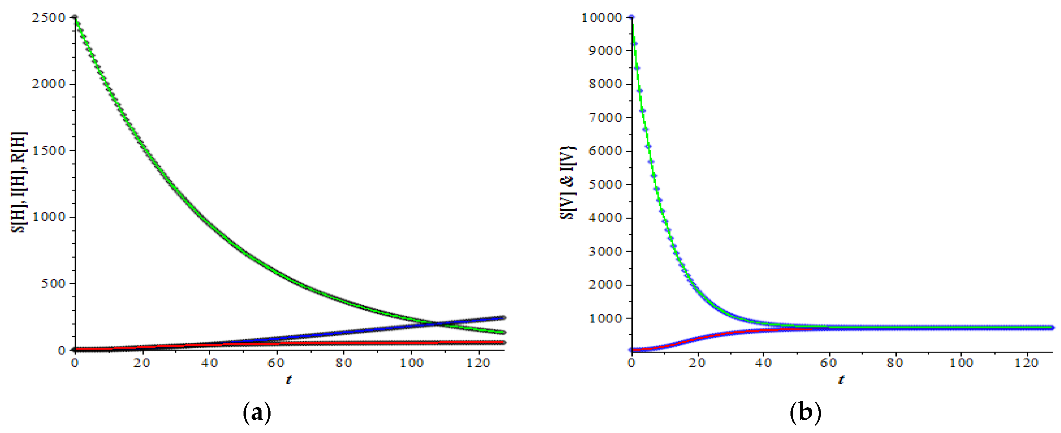
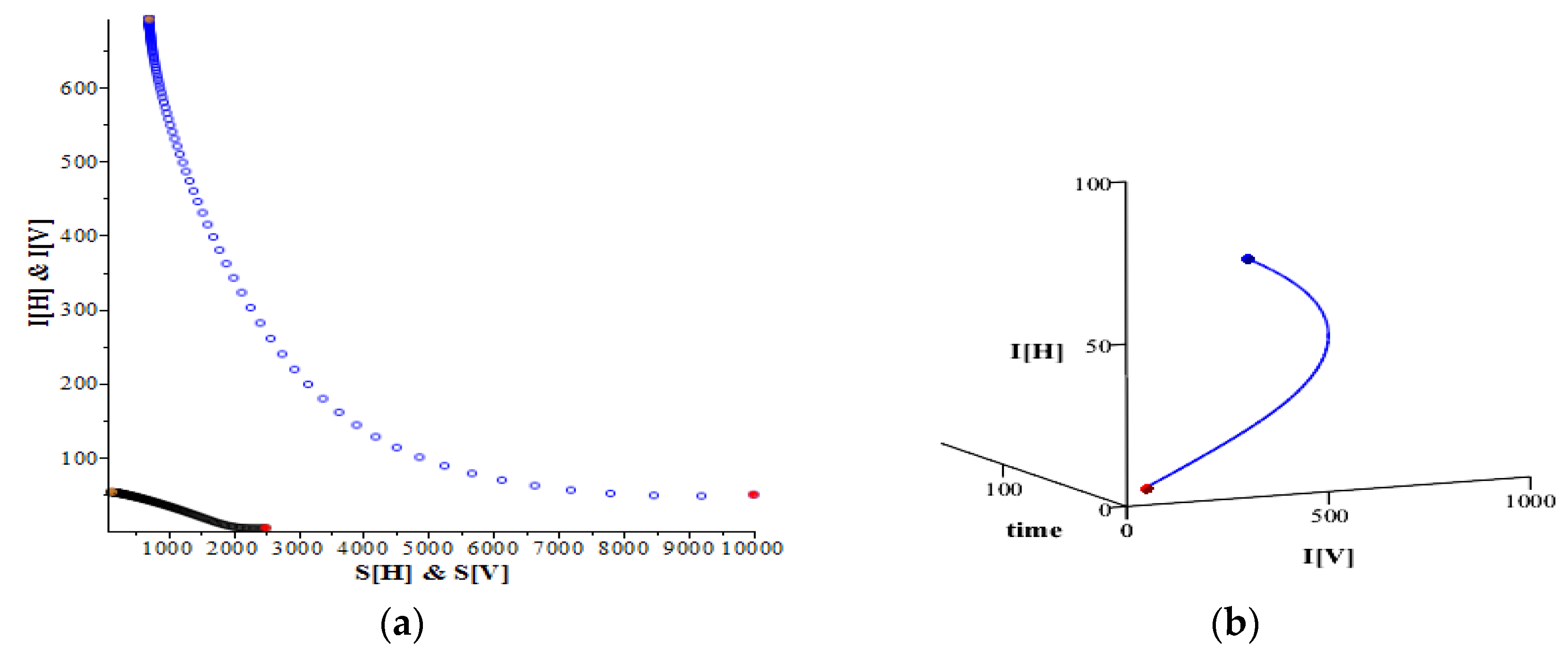
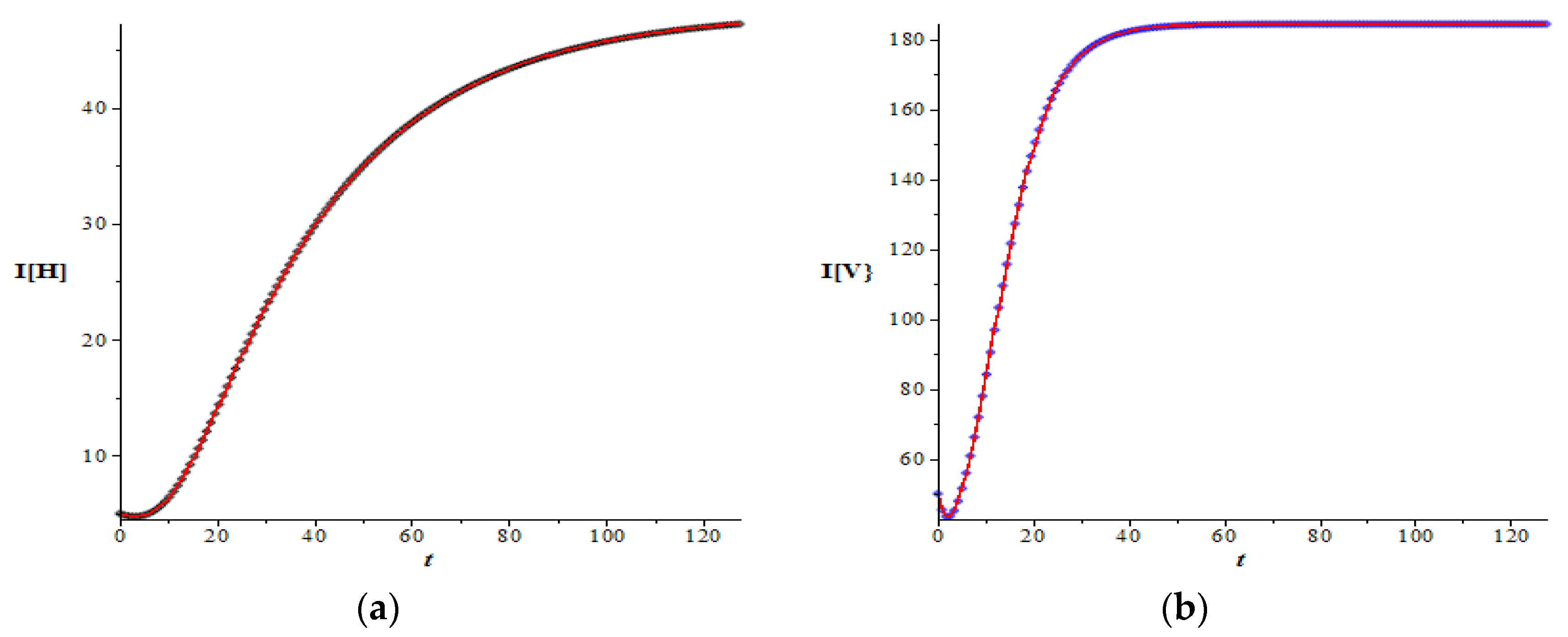
Figure 1 and Figure 2 show the graphs of host and vector dynamics for various combinations of plots resulting from a data set which has an very large basic reproduction number, i.e., R 0 = 166.321. As expected by the theory in the previous section, for this large basic reproduction number, both the number of infected hosts and infected mosquitoes increase as time increases (Figure 1a,b). The increase is more apparent when the figures are zoomed in (Figure 1c,d). Both infected populations approach their non-trivial equilibrium, respectively. Figure 2a shows that the trajectory of these two infective populations travel to approach the equilibrium ( I H * , I V * ) = (53.7291…, 708.6784…). Figure 2b reveals the same case by showing the trajectory of these two infective populations in a 3D graph.
For the second example, we present the dynamics of the dengue transmission system with a medium value of the basic reproduction number, i.e., R 0 = 2.772. The results can be seen in Figure 3 and Figure 4.
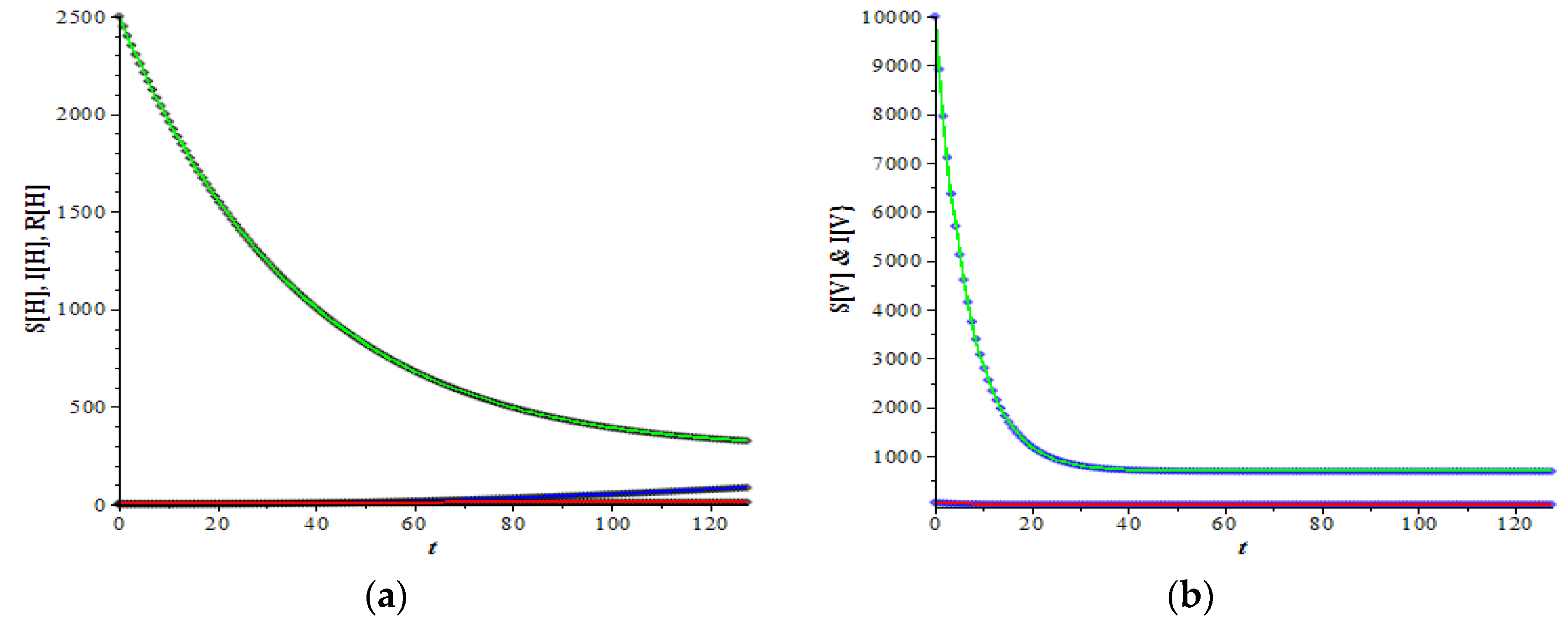
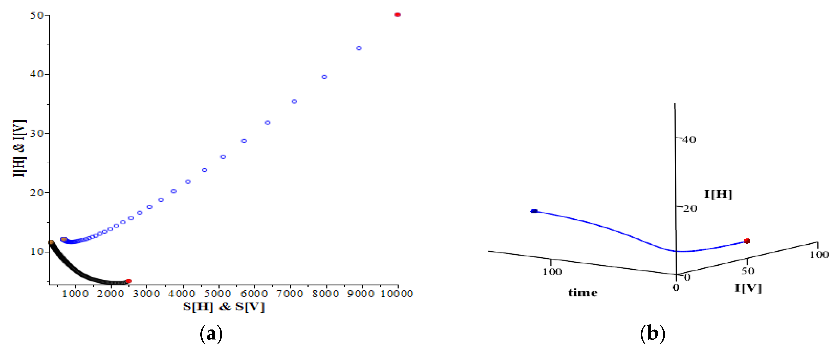
Figure 3 and Figure 4 show the graphs of the host and vector dynamics for various combinations of plots resulting from a data set which has a medium basic reproduction number, i.e., R 0 = 2.772. Compared to the similar graphs in Figure 1 and Figure 2, where both the infective host and infective vector increase as time increases, here only the infective host increases (Figure 3c), while the vector decreases from a relatively high number initial value to a lower value (Figure 3d). Figure 4a shows that the trajectory of these two infective populations travel to approach the equilibrium ( I H * , I V * )   = (11.5844…, 12.0701…). Clearly the number of infective hosts only increase a relatively small amount from 5 to 11, while the infective mosquito number goes down from 50 to 12. This is due to the small rate of infection for the mosquitoes ( β V = 0.0005) compared to that in the previous example ( β V = 0.0075), together with the increase in the mortality rate ( γ V = 1/7) compared to that in the previous example ( γ V = 1/14). This result is expected by the theory in the previous section. Figure 4b reveals the same case by showing the trajectory of these two infective populations in a 3D graph.
The next example is the dynamic of dengue transmission in which the basic reproduction number is very small, given by the last data set in Table 1. In this case, the basic reproduction number is R 0 = 0.042. In line with the theory presented in the previous section, in this case both of the infective populations do not increase at all (Figure 5). Figure 6 also reveals the same results for this very small basic reproduction number.

4.1. The Effect of Vaccination

In this section, we take into account vaccination and the introduction of wolbachia infection into the previous model. Here, it is assumed that, in the host population, a portion p of them is vaccinated at birth, then the number of the susceptible host population at time t in (4) changes into
S H t = S ˜ H t + 0 t 1 p X a e t a t β H I V s d s d a .
Assuming that vaccination is perfect, then all vaccinated individuals will be immune and are removed to the vaccination compartment, which has dynamics
P H t = P ˜ H t + 0 t p X a d a .
The number of infected humans is I H t = N H t S H t + P H t , and hence, the number of those who are still infectious is given by
I H t = I ˜ H t + 1 p 0 t X a E a , t , I V ¯ e γ a d a .
The number of individuals in the recovered class can be obtained from N H t S H t P H t I H t , that is,
R H t = R ˜ H t + 1 p 0 t X a E a , t , I V ¯ e γ a ¯ d a ,
The equations for the mosquitoes are the same as in the case of no vaccination, hence the full system of the age-structured host-vector dengue model is given by Equations (26)–(29), (8) and (9). Using the same argument as before, it can be shown that the effective reproduction number is given by
1 p R 0 ,
where R 0 represents the basic reproduction number. The expression in (30) is often called the effective reproduction number. From the last expression of the effective reproduction number, we conclude that the endemic equilibrium disappears whenever
p > 1 1 R 0 = p c .
The quantity p c can be defined as the critical vaccination level. The value of the critical vaccination level certainly depends on the value of the basic reproduction number. It is well known in many studies that for the case of the direct transmission disease model, we could estimate the threshold number R 0 by using the ratio of life expectancy and mean age at infection. If we choose the survival function to be a negative exponential function, then this estimation is still valid for the indirect transmission model discussed in the previous section [28].
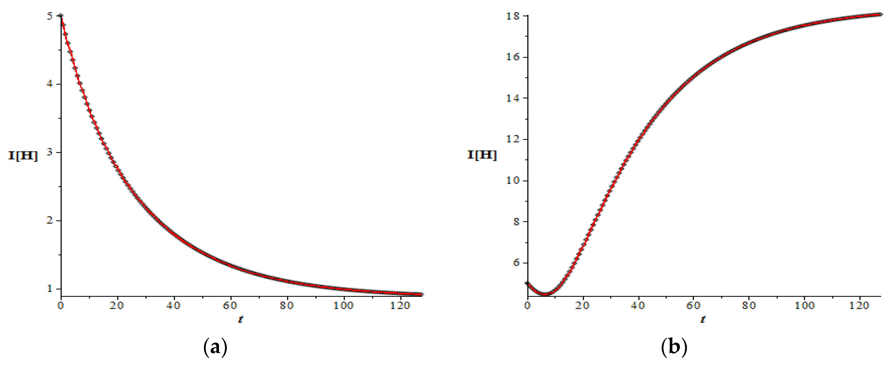
To illustrate the result, let us consider the second data set in Table 1 with the visual solution for the infective populations shown in Figure 7. This data set gives rise to a large basic reproduction number, i.e., R 0 = 41.580. Suppose that we would like to undertake the vaccination of the susceptible population, then according to Equation (31), we need to vaccinate no less than 1 1 41.580 = 0.97595 or 97.595% of the susceptibles. Figure 8a shows the graph of I H t if we vaccinate 98% of the susceptibles, resulting in the elimination of the infective population, and Figure 8b shows the graph of I H t if we vaccinate only 60% of the susceptibles (less than 97.595%), resulting in only a partial decrease in the infective population. These figures agree with the theory discuss above.

4.2. Decaying Effect of Vaccination

In this section, we consider a vaccination with a decaying effect. As before, it is assumed that the host population is vaccinated at birth, as much as p portion, and is removed to the immune class P H . However, it is also assumed that the vaccination has a decaying effect where e τ a is the survival from losing immunity of an individual of age a . Hence, the number of immune individuals at time t is given by
P H t = P ˜ H t + 0 t p X a e τ a d a .
Individuals that lose immunity go back to the susceptible class, which now has dynamics
S H t = S ˜ H t + 0 t 1 p X a E a , t , I V d a + 0 t 1 e τ a p X a E a , t , I V d a .
The number of infected humans can be computed either from the relation I H t = N H t S H t P H t or straight forward by looking at the number of susceptibles who are infected, no longer in the susceptible class (33), and still infectious, that is
I H t = I ˜ H t + 0 t 1 p X a E a , t , I V ¯ e γ a d a            + 0 t e γ a ¯ p X a E a , t , I V ¯ e γ a d a                = I ˜ H t + 0 t e γ a p ¯ X a E a , t , I V ¯ e γ a d a .
The equation for the infected mosquitoes, I V t , remains as in (9). Using the same argument as before, it can be shown that the equilibrium points I H * and I V * are given by
I H * = 0 1 e τ a p X a 1 e β H I V * a e γ a d a            = 0 X a 1 e β H I V * a e γ a d a              0 e τ a p X a 1 e β H I V * a e γ a d a ,
Which, by considering 16 , will give the effective reproduction number
R τ = R 0 p R 1 ,
where R 0 is the basic reproduction number and R 1 = β H β V 0 a X a 0 a Y a d a e γ + τ a d a .
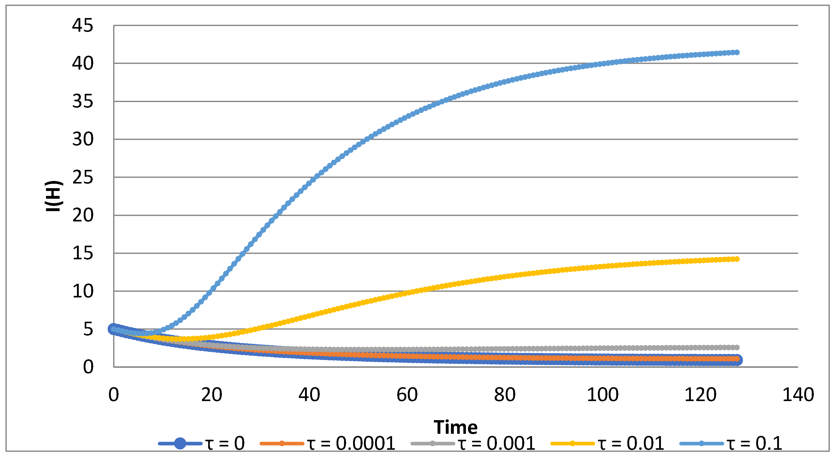
Let us see two extreme conditions in the last expression, i.e., when the rate of losing immunity is relatively low and relatively high. Note that if τ 0     if   the   rate   of   losing   immunity   is   relatively   low ,   then we can ignore the presence of decaying immunity, since the minimum level of vaccination p remains the same as before, that is, p > 1 1 R 0 . However, if τ (the rate of losing immunity is sufficiently high), then the reduction in the value of the basic reproduction number R 0 could be negligible, no matter how large the vaccination rate p is. However, in general, the value of the waning immunity lies in between those two extreme values. In this case, to eliminate the disease, we need R τ < 1 or equivalently p > R 0 1 R 1 , in which the inequality p > R 0 1 R 1 > R 0 1 R 0 holds. This indicates that we may underestimate the critical vaccination level p , if we ignore the presence of decaying immunity, which may consequently result in failing to eliminate the disease. As an illustration we plot the graphs of human infected population for various decaying rates of vaccination (Figure 9). The figure shows the effect of the decaying vaccination for different decay rates for the graphs of human infective population I_H (t) if 98% of the susceptibles are vaccinated. In the absence of decaying effects, this rate of vaccination could drive the infective population to extinction (Figure 8a). However, in the presence of 10% of decaying effects, vaccination has almost no effect in reducing the infective human population.

4.3. The Effect of Wolbachia Infection in the Basic Reproduction Number

In the previous sections we have assumed that there is a natural population of mosquitoes, i.e., there is no wolbachia infection in the mosquitoes. We have assumed that the recruitment rate for the mosquitoes is B V with a natural death rate μ V . Let us also assume that β H and β V are the disease transmission probabilities from vector to host and from host to vector, respectively.
Now we assume that the life span of mosquitoes is reduced by wolbachia infection. This is equivalent to saying that wolbachia infection makes the death rate of the mosquitoes increase. Hence, in the presence of wolbachia infection, the natural death rate μ V changes into a larger rate μ V * , say μ V * = ζ μ V > μ V with ζ > 1 . The constant ζ can be interpreted as a magnification factor of the natural mortality rates μ V . Here, μ V (and so μ V * ) is the parameter of the survival function Q V a . Recall that the basic reproduction number is given by R 0 = B H β H 0 a Q H a e γ a d a   B V β V 0 a Q V a d a , or if we write down the parameter μ V explicitly, we have R 0 μ V = B H β H 0 a Q H a e γ a d a   B V β V 0 a Q V a ; μ V d a in the absence of wolbachia and by following the same calculation in the derivation of Equation (19), in the presence of wolbachia we have R 0 μ V * = B H β H 0 a Q H a e γ a d a   B V β V 0 a Q V a ; μ V * d a . Note that the ratio of R 0 μ V ) R 0 ( μ V * is given by 0 a Q V a ; μ V d a 0 a Q V a ; μ V * d a .
Next, we assume that the transmission probability is reduced by wolbachia infection. Hence, in the presence of wolbachia infection, the natural transmission rates β H and β V change into smaller rates β H *   and β V * , say β H * = ξ β H < β H and β V * = ξ β V < β V with ξ < 1 . The constant ε can be interpreted as a reduction factor of the natural transmission rates β H and β V . As before, recall that for the basic reproduction number if we write down the parameter μ V ,   β H and β V explicitly we have R 0 μ V ; β H ; β V = B H β H 0 a Q H a e γ a d a   B V β V 0 a Q V a ; μ V d a in the absence of wolbachia and by following the same calculation in the derivation of Equation (19), in the presence of wolbachia we have R 0 μ V * ,   β H * , β V * = B H β H * 0 a Q H a e γ a d a   B V β V * 0 a Q V a ; μ V * d a . Note that the ratio of R 0 μ V ; β H ; β V R 0 μ V * ,   β H * , β V * is given by β H β V 0 a Q V a ; μ V d a β H * β V * 0 a Q V a ; μ V * d a .
Now we look at specific survival functions, namely Q H a = e μ H a and Q V a = e μ V a , which mimic the survival rates for humans and mosquitoes, respectively. Consequently, the reproduction number is given by R 0 μ V ,   β H , β V = B H β H μ H + γ 2 B V β V μ V 2 in the absence of wolbachia and R 0 μ V * ,   β H * , β V * = B H ξ β H μ H + γ 2 B V ξ β V ζ μ V 2 in the presence of wolbachia, so that
R 0 μ V ; β H ; β V R 0 μ V * ,   β H * , β V * = ζ ξ 2 > 1
which shows that there is a significant reduction of the basic reproduction number when the wolbachia infected mosquito presence replaces the natural mosquitoes.
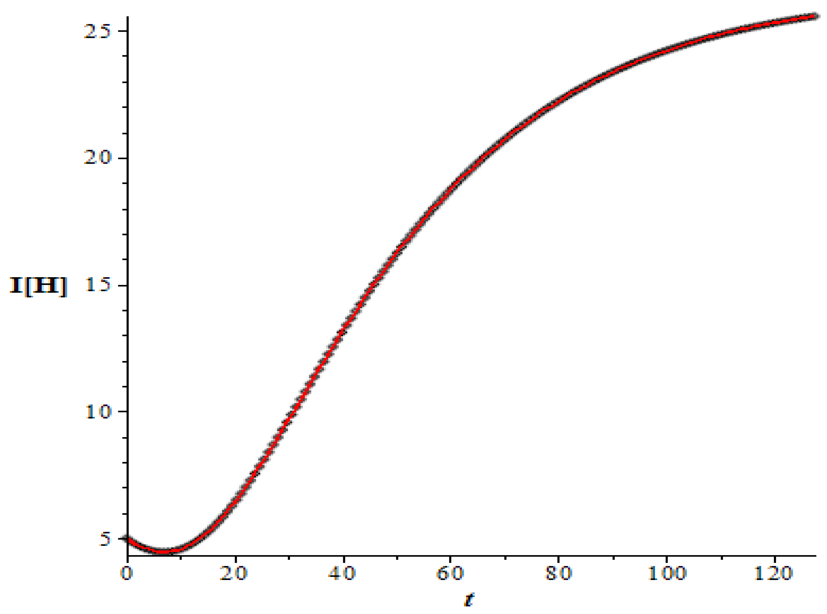
An example can be seen in [29], which agrees with the belief in the effectiveness of wolbachia introduction in controlling the disease. Now, let us consider another example by considering the first data set in Table 1, which has μ V = 1 14 ,   β H = 0.0005 , and β V = 0.0075 . Suppose that the presence of wolbachia could force an increase in the mortality rate to μ V * = 1 / 7 , then in this case ζ = 2 . Moreover, let us assume that the presence of wolbachia also decreases the mosquito infection rate due to proboscis damage to half of the current infection rate, i.e., β V * = 0.00375 and β H * = 0.00025 , or equivalently ξ = 1 / 2 . Then, we have the resulting graph for the human infective population, as presented in Figure 10, with the effective reproduction number 10.395. The number of human infective is almost half of the original number in the absence of wolbachia (Figure 1c). The original basic reproduction number is 166.321. Hence the ratio between the original basic reproduction number and the effective reproduction number in the presence of wolbachia is 16.0000962, which is almost exactly the same as ζ ξ 2 = 2 1 / 2 2 =16. The error is due to the rounding off during the computation. As another example, if we know that the natural basic reproduction number is eight as in [28], then the introduction of wolbachia infection to the mosquitoes could reduce the biting rate by half and increase the mosquito death rate by half of its current level, and theoretically this will make the disease die out. From Equation (31), in the absence of waning immunity, we need to vaccinate at least 87.5 % of the total human population. However, in the presence of waning immunity, then from Equation (36) the vaccination coverage should be much larger than 87.5 % .

5. Conclusions

In this paper a mathematical model of dengue disease transmission has been developed. The model captures the current practice of novel intervention to control dengue transmission, i.e., the introduction of wolbachia infection into mosquitoes. The trivial disease-free and non-trivial endemic equilibria are found, and their stabilities were also analyzed. The existence and the stability of the endemic equilibrium is characterized by a threshold number R 0   as a basic reproduction number, in which the endemic equilibrium exists and is stable whenever R 0 > 1 and it disappears otherwise. The model shows the introduction of wolbachia as one prospective intervention in controlling dengue transmission. The model is able to give the explicit expression of the basic reproduction number of the disease and also is able to show the effect of wolbachia introduction into this number. A simple formula for this effect has been created, by which we can derive some precaution insights regarding the disease dynamics in the presence of the wolbachia intervention program. We found some results and insights regarding the effect of wolbachia into the basic reproduction numbers of dengue. However, the result here is only a rough estimate. We have made a strict assumption in which the replacement of natural mosquitoes by wolbachia infected mosquitoes is certainly possible, hence the analysis is carried out by comparing the absence of wolbachia (100% natural mosquitoes) and the presence of wolbachia (100% natural mosquitoes replaced by the wolbachia infected mosquitoes). Considering the complexity of the real system, a more realistic model should take into account these complexities into the transmission mechanism, such as the explicit transmission of the mosquitoes and age-structured meeting rate [50]. A more realistic wolbachia transmission also might alter the conclusion in this paper into a more prudent prediction. This work is currently under investigation.

Author Contributions

Conceptualization, methodology, formal analysis, writing—original draft preparation: A.K.S. and E.S.; writing—review and editing, investigation, interpretation: A.K.S., B.G. and H.H.; data curation: H.H; project administration: A.K.S.; resources, funding acquisition: Y.P. and E.N. All authors have read and agreed to the published version of the manuscript.

Funding

We thank the University of Padjadjaran and the Indonesian Government who funded the work through the scheme “Riset Kolaborasi Indonesia 2022”, contract number 2203/UN6.3.1/PT.00/2022.

Institutional Review Board Statement

Not applicable.

Conflicts of Interest

The authors declare no conflict of interest.

Appendix A

We will show that 0 R 1 a d a 0 R 2 a d a < 1 . It is known that R 1 a = B H Q H a e β H I V * a β H a e γ a and R 2 a = B V Q V a e β V I H * a β V   a . Let us define
g x , y = g 1 x g 2 y ,
with
g 1 x = β H 0 e γ a X a e β H I V * a 1 e β H a x β H x d a ,
g 2 y = β V 0 Y a e β V I H * a 1 e β V a y β H y d a .
By inspecting their first derivatives, g 1 and g 2 are decreasing functions of x and y respectively. We note that
g 0 , 0 = β H 0 X a e β H I V * a a e γ a d a β V 0 Y a e β V I H * a a   d a = 0 R 1 a d a 0 R 2 a d a ,
and
g I V * , I H * = B H β H 0 Q H a e γ a 1 e β H I V * a β H I V * d a B V β V 0 Q V a 1 e β V I H * a β V I H * d a         = B H 0 Q H a e γ a 1 e β H I V * a I V * d a B V 0 Q V a 1 e β V I H * a I H * d a = 1 1 = 1
Since g is a decreasing function both in x and y variables, then g 0 , 0 < g I V * , I H * , and hence proves the assertion that 0 R 1 a d a 0 R 2 a d a < 1 .

Appendix B

We will show that Lemma 2 still holds if the condition 0 R j a d a < 1 is replaced by a weaker condition 0 R i a d a 0 R j a d a < 1 . The proof goes as follows. Let K j = sup 0 s f j s with j 1 , 2 . For every ϵ < 0 choose T j large enough so that T j R j a d a < ϵ and f j 0 t < ϵ if t > T j . If T = max T 1 , T 2 then T R j a d a < ϵ , and if i ,   j 1 , 2 with i j then we have
T t sup t a s t f i s R j a d a T t sup 0 s t f i s R j a d a = sup 0 s t f i s T t R j a d a ϵ sup 0 s t f i s = ϵ K i .
0 T sup t a s t f i s R j a d a 0 T sup t T s t f i s R j a d a = sup t T s t f i s 0 T R j a d a sup t T s f i s 0 R j a d a .
For every t > T , the last two inequalities alter the inequalities in the hypothesis of Lemma 2 into
f j s ϵ + ϵ K i + sup t T s f i s 0 R j a d a .
Since this holds for every t > T , if t > 2 T , then we have
sup t T s f 1 s ϵ + ϵ K 2 + sup t T s f 2 s 0 R 1 a d a ,
sup t T s f 2 s ϵ + ϵ K 1 + sup t T s f 1 s 0 R 2 a d a .
Hence,
sup t T s f 1 s 2 ϵ + ϵ K 1 + K 2 + sup t T s f 1 s 0 R 2 a d a 0 R 1 a d a .
Moreover, by defining K = max K 1 , K 2 we have
sup t T s f 1 s 1 0 R 1 a d a 0 R 2 a d a 2 ϵ + K ϵ = 2 + K ϵ .
Finally, since 0 R 1 a d a 0 R 2 a d a < 1 , and by considering sup t T s f 1 s is less than or equals to 2 + K ϵ 1 0 R 1 a d a 0 R 2 a d a   we can make sup t T s f 1 s arbitrary small, which shows that lim t f 2 t = 0 . The conclusion that lim t f 1 t = 0 can be reached by a similar argument.

References

  1. Gubler, D.J. Epidemic dengue/dengue hemorrhagic fever as a public health, social and economic problem in the 21st century. Trends Microbiol. 2002, 10, 100–102. [Google Scholar] [CrossRef]
  2. Newton, E.A.C.; Reiter, P. A Model of the Transmission of Dengue Fever with an Evaluation of the Impact of Ultra-Low Volume (ULV) Insecticide Applications on Dengue Epidemics. Am. J. Trop. Med. Hyg. 1992, 47, 709–720. [Google Scholar] [CrossRef] [PubMed] [Green Version]
  3. Clarke, T. Breakbone fever. Nature 2002, 416, 672–674. [Google Scholar] [CrossRef] [PubMed]
  4. Kinney, R.M.; Huang, C.Y. Development of new vaccines against dengue fever and Japanese encephaliptis. Intervirology 2001, 44, 176–197. [Google Scholar] [CrossRef] [PubMed]
  5. Abual-Rub, M.S. Vaccination in a model of an epidemic. Int. J. Math. Math. Sci. 1998, 23, 425–429. [Google Scholar] [CrossRef] [Green Version]
  6. Anderson, R.M. Infectious Disease of Humans: Dynamics and Control; Oxford University Press: Oxford, UK, 1992. [Google Scholar]
  7. Esteva, L.; Vargas, C. Analysis of a dengue disease transmission model. Math. Biosci. 1998, 150, 131–151. [Google Scholar] [CrossRef]
  8. Feng, Z.; Velasco-Hernandez, Z.X. Competitive exclusion in a vector-host model for the dengue fever. J. Math. Biol. 1997, 35, 523–544. [Google Scholar] [CrossRef] [Green Version]
  9. Soewono, E.; Supriatna, A.K. A two-dimensional model for transmission of dengue fever disease. Bull. Malays. Math. Sci. Soc. 2001, 24, 49–57. [Google Scholar]
  10. Soewono, E.; Supriatna, A.K. A paradox of vaccination predicted by a simple dengue disease model. In Industrial Mathematics; Joshi, M.C., Pani, A.K., Sabnis, S.V., Eds.; Narosa Publishing House: New Delhi, India, 2006; pp. 459–470. [Google Scholar]
  11. Calsina, À.; Saldana, J. Basic theory for a class of models of hierarchically structured population dynamics with distributed states in the recruitment. Math. Model. Methods Appl. Sci. 2006, 16, 1695–1722. [Google Scholar] [CrossRef]
  12. Arino, O.; Smith, W.V. Migration in age structured population dynamics. Math. Model. Methods Appl. Sci. 1998, 8, 905–925. [Google Scholar] [CrossRef]
  13. Kirkilionis, M.A.; Diekmann, O.; Lisser, B.; Nool, M.; Sommeijer, B.; De Roos, A.M. Numerical Continuation of Equilibria of Physiologically Structured Population Models I: Theory. Math. Model. Methods Appl. Sci. 2001, 11, 1101–1127. [Google Scholar] [CrossRef]
  14. Martcheva, M.; Pilyugin, S.S. An Epidemic Model Structured by Host Immunity. J. Biol. Syst. 2006, 14, 185–203. [Google Scholar] [CrossRef]
  15. Mischler, S.; Perthame, B.; Ryzhik, L. Stability in a Nonlinear Population Maturation Model. Math. Model. Methods Appl. Sci. 2002, 12, 1751–1772. [Google Scholar] [CrossRef] [Green Version]
  16. Webb, G.F. Population models, structured by age, size, and spatial position. In Structured Population Models in Biology and Epidemiology; Springer: Berlin/Heidelberg, Germany, 2008; Volume 1936, pp. 1–49. [Google Scholar]
  17. Gabriel, P.; Garbett, S.P.; Quaranta, V.; Tyson, D.R.; Webb, G.F. The contribution of age structure to cell population responses to targeted therapeutics. J. Theor. Biol. 2012, 311, 19–27. [Google Scholar] [CrossRef] [Green Version]
  18. Webb, G.F. Theory of nonlinear age-dependent population dynamics. In Chapman and Hall Pure and Applied Mathematics (Book 89); CRC Press: Boca Raton, FL, USA, 1985; 312p. [Google Scholar]
  19. Brauer, F. A model for an SI disease in an age—Structured population. Discret. Contin. Dyn. Syst. Ser. B 2002, 2, 257–264. [Google Scholar] [CrossRef]
  20. Gyilenberg, M.; Webb, G.F. A nonlinear structured population model of tumor growth with quiescence. J. Math. Biol. 1990, 28, 671–694. [Google Scholar] [CrossRef]
  21. Inaba, H. Threshold and stability results for an age-structured epidemic model. J. Math. Biol. 1990, 28, 411–434. [Google Scholar] [CrossRef]
  22. Müller, J. Optimal Vaccination Patterns in Age-Structured Populations. SIAM J. Appl. Math. 1998, 59, 222–241. [Google Scholar] [CrossRef]
  23. Müller, J. Optimal vaccination patterns in age-structured populations: Endemic case. Math. Comput. Model. 2000, 31, 149–160. [Google Scholar] [CrossRef]
  24. Pongsumpun, P.; Tang, I. Transmission of dengue hemorrhagic fever in an age structured population. Math. Comput. Model. 2003, 37, 949–961. [Google Scholar] [CrossRef]
  25. Supriatna, A.; Soewono, E.; van Gils, S. A two-age-classes dengue transmission model. Math. Biosci. 2008, 216, 114–121. [Google Scholar] [CrossRef] [PubMed]
  26. Tasman, H.; Supriatna, A.K.; Nuraini, N.; Soewono, E. A Dengue Vaccination Model for Immigrants in a Two-Age-Class Population. Int. J. Math. Math. Sci. 2012, 2012, 236352. [Google Scholar] [CrossRef] [Green Version]
  27. Brauer, F. The Analysis of Some Characteristic Equations Arising in Population and Epidemic Models. J. Dyn. Differ. Equ. 2004, 16, 441–453. [Google Scholar] [CrossRef]
  28. Supriatna, A.K. Estimating the basic reproduction number of dengue transmission during 2002–2007 outbreaks in Bandung–Indonesia. WHO Dengue Bull. 2009, 33, 21–33. [Google Scholar]
  29. Supriatna, A.K. Dengue transmision model with age-dependent survival rates in the presence of wolbachia infection. In Latest Advances in System Science and Computational Intellegence; Academia: San Francisco, CA, USA, 2012; pp. 216–218. ISBN 978-1-61804-094-7. [Google Scholar]
  30. McMeniman, C.J.; Lane, R.V.; Cass, B.N.; Fong, A.W.; Sidhu, M.; Wang, Y.F.; O’Neill, S.L. Stable introduction of a life-shortening Wolbachia infection into the mosquito Aedes aegypti. Science 2009, 323, 141–144. [Google Scholar] [CrossRef] [PubMed] [Green Version]
  31. Mullard, A. Bacteria Could Help Control Dengue Fever; Nature: Berlin, Germany, 2009. [Google Scholar]
  32. Turley, A.P.; Moreira, L.A.; O’Neill, S.; McGraw, E.A. Wolbachia Infection Reduces Blood-Feeding Success in the Dengue Fever Mosquito, Aedes aegypti. PLoS Negl. Trop. Dis. 2009, 3, e516. [Google Scholar] [CrossRef]
  33. Hethcote, H.W.; Tudor, D.W. Integral equation models for endemic infectious diseases. J. Math. Biol. 1980, 9, 37–47. [Google Scholar] [CrossRef]
  34. Diekmann, O.; Heesterbeek, J.A.P.; Metz, J.A.J. On the definition and the computation of the basic reproduction ratio R 0 in models for infectious diseases in heterogeneous populations. J. Math. Biol. 1990, 28, 365–382. [Google Scholar] [CrossRef] [Green Version]
  35. Diekmann, O.; Heesterbeek, J.A.P. Mathematical Epidemiology of Infectious Diseases; John Wiley & Son: Hoboken, NJ, USA, 2000. [Google Scholar]
  36. Driessche, P.V.D.; Watmough, J. Reproduction numbers and sub-threshold endemic equilibria for compartmental models of disease transmission. Math. Biosci. 2002, 180, 29–48. [Google Scholar] [CrossRef]
  37. Supriatna, A.K.; Soewono, E. Gronwall-like inequality and its application in epidemic modeling. In Proceedings of the 2nd IMT-GT Regional Conference in Mathematics, Statistics and Their Applications, Penang, Malaysia, 13–15 June 2006. [Google Scholar]
  38. Hutson, V.; Schmitt, K. Permanence and the dynamics of biological systems. Math. Biosci. 1992, III, 1–71. [Google Scholar] [CrossRef]
  39. Lewontin, R. The meaning of stability. Brookhaven Symp. Biol. 1975, 22, 13–24. [Google Scholar]
  40. Teng, Z.D.; Li, Z.M.; Jiang, H.J. Pemanence criteria in non-autonomous predator–prey Kolmogorov systems and its applications. Dyn. Syst. 2004, 19, 171–194. [Google Scholar] [CrossRef]
  41. Burden, R.L.; Faires, J.D. Numerical Analysis, 8th ed.; Thomson Brooks/Cole: Belmont, CA, USA, 2005. [Google Scholar]
  42. Burton, T.A. Volterra Integral and Differential Equations, 2nd ed.; Mathematics in Science & Engineering; Elsevier: Amsterdam, The Netherlands, 2005; Volume 202. [Google Scholar]
  43. Jerri, A.J. Introduction to Integral Equations with Applications; Pure & Applied Mathematics; Marcel Dekker: New York, NY, USA, 1985; Volume 93. [Google Scholar]
  44. Linz, P. Analytical and Numerical Methods for Volterra Equations; Studies in Applied Mathematics 7; SIAM: Philadelphia, PA, USA, 1985. [Google Scholar]
  45. Becker, L.C.; Wheeler, M. Numerical and Graphical Solutions of Volterra Integral Equations of the Second Kind; Christian Brothers University: Memphis, TN, USA, 2005. [Google Scholar]
  46. Macrotrend. Available online: https://www.macrotrends.net/countries/IDN/indonesia/fertility-rate (accessed on 24 June 2022).
  47. Nuraini, N.; Fauzi, I.S.; Fakhruddin, M.; Sopaheluwakan, A.; Soewono, E. Climate-based dengue model in Semarang, Indonesia: Predictions and descriptive analysis. Infect. Dis. Model. 2021, 6, 598–611. [Google Scholar] [CrossRef]
  48. Götz, T.; Altmeier, N.; Bock, W.; Rockenfeller, R.; Sutimin; Wijaya, K.P. Modeling dengue data from Semarang, Indonesia. Ecol. Complex. 2017, 30, 57–62. [Google Scholar] [CrossRef]
  49. Naksathit, A.T.; Scott, T.W. Effect of female size on fecundity and survivorship of Aedes aegypti fed only human blood versus human blood plus sugar. J. Am. Mosq. Control Assoc. 1998, 14, 148–152. [Google Scholar]
  50. Greenhalgh, D. Threshold and Stability Results for an Epidemic Model with an Age-Structured Meeting Rate. Math. Med. Biol. A J. Ima 1988, 5, 81–100. [Google Scholar] [CrossRef]
Figure 1. (a) shows the graphs of S H t , I H t , and R H t , indicated respectively by green, red, and blue line colors for a very large basic reproduction number ( R 0 = 166.321), while (b) shows the graphs of S V t and I V t , indicated by green and purple line color for the same parameters as in (a). (c,d) provides a zoomed in version of I H t and I V t graphs.
Mathematics 10 03950 g001aMathematics 10 03950 g001b
Figure 2. The phase port of S H t and I H t (black) and the phase port of S V t   I V t (blue) are shown in (a). (b) shows the trajectory of I H t and I V t in a 3D graph. The red dots in both figures indicate the initial values of the system. The parameters are the same as in Figure 1.
Mathematics 10 03950 g002
Figure 3. (a) shows the graphs of S H t , I H t , and R H t , while (b) shows the graphs of S V t and I V t with the explanation as in Figure 1. To compare the number of infected humans and mosquitoes, we plot I H t in (c) and I V t in (d). Here, we use the data set which has a medium basic reproduction number, i.e., R 0 = 2.772.
Mathematics 10 03950 g003aMathematics 10 03950 g003b
Figure 4. The phase port of S H t and I H t (black) and the phase port of S V t   I V t (blue) are shown in (a). (b) shows the trajectory of I H t and I V t in a 3D graph. The red dots in both figures indicate the initial values of the system. The parameters are the same as in Figure 3.
Mathematics 10 03950 g004
Figure 5. (a) shows the graphs of S H t , I H t , and R H t . To compare the number of infected humans and mosquitoes, we plot I H t in (c) and I V t in (d), while (b) plots them in one frame. Here, we use the data set which has a very small basic reproduction number, i.e., R 0 =   0.042.
Mathematics 10 03950 g005
Figure 6. The phase port of S H t and I H t (black) and the phase port of S V t   I V t (blue) are shown in (a). (b) shows the trajectory of I H t and I V t in a 3D graph. The red dots in both figures indicate the initial values of the system. The parameters are the same as in Figure 5.
Mathematics 10 03950 g006
Figure 7. (a) shows the graphs of I H t , while (b) shows the graphs of I V t . Here we use the data set which gives a large basic reproduction number, i.e., R 0 =   41.580 (without the presence of vaccination).
Mathematics 10 03950 g007
Figure 8. (a) shows the graphs of I H t if 98% of the susceptibles are vaccinated, while (b) shows the graphs of I H t if only 60% of the susceptibles are vaccinated. In the former, the resulting effective reproduction number is 0.832, while, in the latter, the resulting effective reproduction number is 16.632.
Mathematics 10 03950 g008
Figure 9. The figure shows the effect of the decaying vaccination for different decay rates for the graphs of human infective population I H t if 98% of the susceptibles are vaccinated.
Mathematics 10 03950 g009
Figure 10. The figure shows the graphs of human infective population I H t when there is a replacement of natural mosquitoes by the population of wolbachia infected mosquitoes, assuming there is a decrease of infection rates in data set 1 in Table 1 to half of the original rates, and an increase of mosquito mortality rate in data set 1 in Table 1 to double the original mortality rate.
Mathematics 10 03950 g010
Table 1. Parameter values used in the numerical examples.
Parameter Very Large R 0 Large R 0 Medium R 0 Small R 0 Very Small
R 0
μ H 3.7915 × 10⁻⁵ [28]3.7915 × 10−53.7915 × 10−53.7915 × 10−53.7915 × 10−5
μ V 1/141/71/71/71/7
B H 2.52 [46]2.522.522.522.52
B V 100 [49]100100100100
β H 0.00050.00050.00050.00010.00005
β V 0.00750.00750.00050.00010.00005
γ 1/30 [47,48]1/301/301/301/30
S H 0 25002500250025002500
I H 0 55555
R H 0 00000
S V 0 10,00010,00010,00010,00010,000
I V   0 5050505050
R 0 166.32141.5802.7720.1110.042
Publisher’s Note: MDPI stays neutral with regard to jurisdictional claims in published maps and institutional affiliations.