Analytical Solution for Controlled Drug Release with Time-Dependent Diffusion Parameter

Abstract

Drugs seem to diffuse in different manners in a delivery device due to the increment of the device pore size during swelling. However, the diffusion parameter, D, is often assumed constant. In this work, a new developed controlled drug release model with a time-dependent diffusion parameter is compared to one- and two-phase models. The new model was obtained as an improvement of the previous constant and piece-wise constants models. The models are developed by solving an advection–diffusion equation using the Landau transformation method and the separation of variables method. To test these models, we fit experimental data by the developed models using the least squares fitting technique. The curve-fitting result shows that the least squares error of the two-phase and the time-dependent models are 10 times smaller than the single-phase model. The CPU time for the time-dependent model is the lowest, showing that a time-dependent model is the best option among all three tested models considering both factors of the determined least squares error and the time consumption.

1. Introduction

Controlled drug delivery has been a topic of interest for researchers from various fields. There is an extensive study on controlled drug delivery particularly in the pharmaceutical and the mathematical fields. Controlled drug delivery systems help to maintain an optimal level of drug concentration in a human’s blood or body system within some time period [1]. This feature of the system manages to restrain the drawbacks of conventional medicine by reducing the drug dosing frequency [2] and thus increasing patient compliance [3].

Micelles, liposomes, hydrogels, vesicles and dendrimers are some of the known drug carriers for controlled drug release [4,5]. The hydrogel is particularly appealing in designing the drug carrier for controlled release [3,6]. Hydrogels are made of a hydrophilic polymer which allows the absorption of a huge amount of fluid [7,8]. Hydrogels also can be moulded into different forms, which can be as nano- or microparticles, slabs, films and coating, depending on the biomedical demands [8]. The hydrogel has the ability to swell and shrink, depending on the current environmental condition to aid the controlled drug release [8].

In addition, the hydrogel is porous in nature [8,9]. The porosity is a good trait that offers a great advantage as a carrier for controlled drug delivery [6,8]. The swelling nature of the porous hydrogel changes the morphology of the pore of the device, thus affecting the mobility of the substances within the device [10]. The swelling also loosens up the polymer chain and thus facilitates the drug diffusion [8]. Thus, the dynamics of the device geometry directly affect the diffusivity of a drug delivery from the device. Previously, we had formulated a model of controlled drug release from a swelling hydrogel considering a phase-wise constant diffusion parameter [11]. The diffusion parameter can be in the form of a constant or as an expression [12,13,14].

The first diffusion model based on free volume theory was proposed by Fujita [15]. The free volume theories assume that the free volume is the major factor controlling the diffusion rate of molecules. In Fujita’s model, the diffusion coefficient is defined as the self-diffusion coefficient of the molecule. Fujita’s model seems adequate in the description of the diffusion of small-sized diffusants in dilute and semi-dilute polymer solutions and gels, mostly organic systems. Gao and Fagerness [16] described diffusivity measurements of drug (adinazolam mesylate) and water in a variety of solutions including polymer gel. In their study, they found that the drug diffusivity in a non-interactive multicomponent system can be described as an exponential function of an additive contribution from each viscosity-inducing agent (VIA) component. Thus, the self-diffusion coefficient of adinazolam was found to depend on the nature of the VIA present in solution as well as on its concentration. Most of the physical models of diffusion for polymer solutions, gels and solids are reviewed in Masaro and Zhu [17]. They summarize the different physical models and theories of diffusion and their uses in describing the diffusion in polymer solutions, gels and even solids. Although the diffusion in polymer systems is a complicated process, various models and theories succeeded in describing the diffusion process under different circumstances and contributed to the understanding of diffusion phenomena.

Aside from our previously formulated model in [11], numerous other mathematical models in the study of controlled drug release had been developed. These models have considered the different forms of the hydrogels [18,19]. The mathematical models keep being improved to implement the real-life events and give a good correlation to the in vivo data [8]. To develop the model, the mechanism of controlled release to be considered must be identified. Fundamentally, there are diffusion-controlled, dissolution-controlled, swelling-controlled and erosion-controlled systems [7,19]. Siepmann and Siepmann [18] had found that drug diffusion plays the predominant step in many cases while the other controlled release mechanisms act as the major role in the process of drug release. In the study of controlled drug release from swelling device, at least, the diffusion- and swelling controlled system must be considered.

One of the early developed mathematical model of controlled drug release is the Higuchi equation [20]. However, this equation is purely diffusion-controlled [21]. The infamous Korsmeyer–Peppas (power law) model had been developed from the Higuchi equation [19]. The power law model is highly used by the researcher owing to its simplicity. Nonetheless, this equation cannot give a detailed explanation of the drug diffusion process in the drug device [22]. This shortcoming of the power law model can be overcome by Fick’s law of diffusion model. Fick’s law model can explicitly explain the diffusion behaviour of drugs in a device without the need of having high numbers of parameters [23]. There is also the advection–diffusion equation that consider both diffusion-controlled and swelling-controlled mechanisms [24]. The computational difficulty for the advection–diffusion equation is also particularly low [25].

Generally, the drug diffusivity, referred to as the drug diffusion parameter, is conveniently considered as constant. In theory, the pore size of a swelling device would increase with time due to the growing boundary of the device. Our previous research [11] also agrees with the theory when it is found that the diffusion parameter shows a dynamic behaviour when the drug release process is assumed to be in two phases. However, previously, the drug diffusion parameter is considered as two different constants that differ in each phase. That study has already given a good result and fits well with the experimental data.

In this paper, the idea of the constant phase-wise diffusion parameter from our previous study [11] is extended to be a parameter that depends on time. Despite the state of the art relating the diffusivity to the hydration of the system as mentioned in the literature, for simplicity of the model, a time-dependent diffusion parameter is used in this study representing the effective diffusivity of the whole process. Similar to our previous paper, the advection–diffusion equation will be employed to develop the controlled drug release model. The model developed by Bierbrauer [7], called the single-phase model, and the previous two-phase model [11] will be redeveloped in this paper. The derivation of the new time dependent model will be shown specifically for the linear swells case. The results for all the three models will be compared.

2. Methodology

For a swelling device, a mathematical equation must comprise the moving boundary together with the diffusion phenomena. The advection–diffusion equation can simultaneously include both. Firstly, consider the general advection–diffusion equation [7,11,26],

$$\frac{\partial c}{\partial t}=\nabla ·\left(D\left(x,t\right)\nabla c\left(x,y,z,t\right)\right)-\nabla ·\left(c\left(x,y,z,t\right)u\left(x,y,z,t\right)\right),$$

(1)

where $c(x,y,z,t)$ is the concentration of drug in the device, $D(x,t)$ is the drug diffusion parameter, and $u(x,y,z,t)$ is the swelling velocity of the device. However, in order to analytically solve this model, the drug release process is only considered to be in a one-dimensional (1D) spatial region [7], and thus Equation (1) reduces to

$$\frac{\partial c}{\partial t}=D\left(x,t\right)\frac{{\partial }^{2}c\left(x,t\right)}{\partial x^2}-\frac{\partial c\left(x,t\right)}{\partial x}u\left(x,t\right)-c\left(x,t\right)\frac{\partial u\left(x,t\right)}{\partial x}$$

(2)

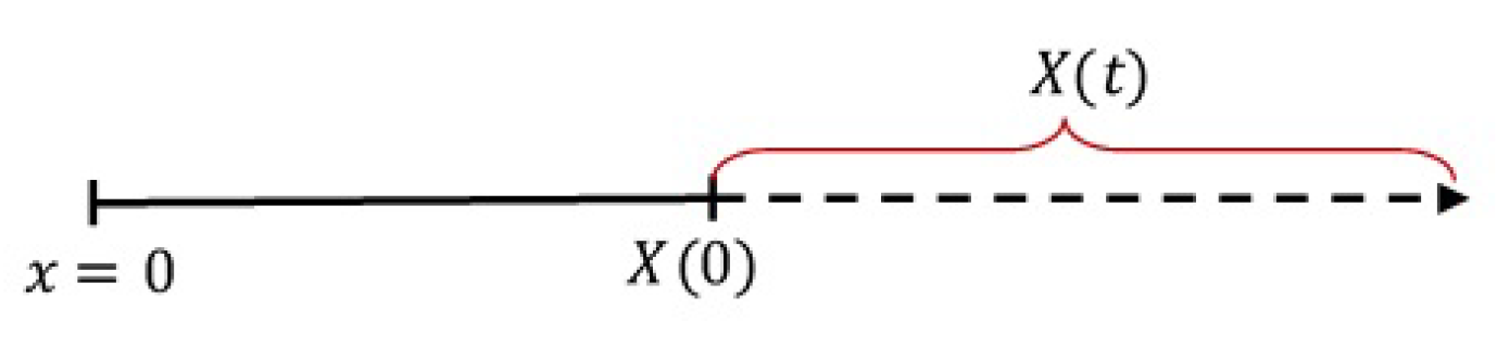
The one-dimensional spatial region considered for Equation (2) can be illustrated as in Figure 1.

In Figure 1, x is the spatial independent variable with $x=0$ representing the device core, $X\left(0\right)$ is the initial boundary of the device, and $X\left(t\right)\ge X\left(0\right)$ is the moving boundary (swelling) of the device at time t, called the device growth function. When the device swells, $X\left(t\right)$ increases as t increases. Thus, in general, the function $X\left(t\right)$ can be represented by a linear, exponential, logistic or any increasing function. In this work, we use the linear growth function as given by [7]

$$X\left(t\right)=L\left(1+gt\right),$$

(3)

where L is the device original radius, and g is the growth factor. This growth factor will be determined using curve fitting with the experimental data, resulting in a suitable linear equation to represent $X\left(t\right)$. It is assumed that the device swelling velocity is uniform satisfying $u(x,t)=\frac{\dot{X}\left(t\right)}{X\left(t\right)}x$ (see [7]). Thus, Equation (2) can be written as

$$\frac{\partial c}{\partial t}=D\left(x,t\right)\frac{{\partial }^{2}c\left(x,t\right)}{\partial x^2}-\frac{\partial c\left(x,t\right)}{\partial x}\left(\frac{\dot{X}\left(t\right)}{X\left(t\right)}x\right)-c\left(x,t\right)\frac{\dot{X}\left(t\right)}{X\left(t\right)}\mathrm{in}0<x<X\left(t\right),t>0.$$

(4)

This equation is subject to some initial and boundary conditions. The initial drug concentration within the device is assumed to be the initial condition, i.e., $c(x,t)=c_0$ for all x within the device geometry. Meanwhile, from previous studies in [7,11], it is assumed that there is no flux at the centre of the device, $\frac{\partial c}{\partial t}(0,t)=0$, $t>0$, and there is no drug present at the boundary of the device, i.e., $c\left(X\right(t),t)=0$, $t>0$. Equation (4) serves as the foundation in developing three different mathematical models of controlled drug release which are the single-phase model, the two-phase model, and the time-dependent model.

2.1. The Single-Phase Model

The single-phase model has been developed in [7] previously. This model is the basic controlled drug release model considering the diffusion parameter as a single constant instead of a function. The advection–diffusion equation with constant D is

$$\frac{\partial c}{\partial t}=D\frac{{\partial }^{2}c\left(x,t\right)}{\partial x^2}-\frac{\partial c\left(x,t\right)}{\partial x}\left(\frac{\dot{X}\left(t\right)}{X\left(t\right)}x\right)-c\left(x,t\right)\frac{\dot{X}\left(t\right)}{X\left(t\right)}\mathrm{in}0<x<X\left(t\right),t>0.$$

(5)

Equation (5) is further transformed to overcome the problem of the time-dependent moving boundary space domain. Therefore, the Landau transformation method is used by introducing two new parameters which are [7]

$$\zeta =\frac{x}{X\left(t\right)},\tau =t.$$

(6)

Derivatives in Equation (5) are transformed using the following chain rules:

$$\frac{\partial c}{\partial t}=-\zeta \frac{\dot{X}\left(\tau \right)}{X\left(\tau \right)}\frac{\partial c}{\partial \zeta }+\frac{\partial c}{\partial \tau },$$

$$\frac{\partial c}{\partial x}=\frac{1}{X\left(\tau \right)}\frac{\partial c}{\partial \zeta },$$

and

$$\frac{{\partial }^{2}c}{\partial x^2}=\frac{1}{X^2\left(\tau \right)}\frac{{\partial }^{2}c}{\partial {\zeta }^2}.$$

Substituting all transformed derivatives into Equation (5) gives the transformed advection–diffusion,

$$-\zeta \frac{\dot{X}\left(\tau \right)}{X\left(\tau \right)}\frac{\partial c}{\partial \zeta }+\frac{\partial c}{\partial \tau }=\frac{D}{X^2\left(\tau \right)}\frac{{\partial }^{2}c}{\partial {\zeta }^2}-\zeta \frac{\dot{X}\left(\tau \right)}{X\left(\tau \right)}\frac{\partial c}{\partial \zeta }-\frac{\dot{X}\left(\tau \right)}{X\left(\tau \right)}c$$

$$\frac{\partial c}{\partial \tau }=\frac{D}{X^2\left(\tau \right)}\frac{{\partial }^{2}c}{\partial {\zeta }^2}-c\frac{\dot{X}\left(\tau \right)}{X\left(\tau \right)}\mathrm{in}0<x<X\left(\tau \right),\tau >0$$

(7)

with the following transformed initial and boundary conditions:

$$\begin{array}{c}c\left(\zeta ,0\right)=c_0 \mathrm{in} 0<\zeta <1,\hfill \\ \frac{\partial c}{\partial \zeta }(0,\tau )=0,\tau >0,\hfill \\ c(1,\tau )=0,\tau >0.\hfill \end{array}$$

Equation (7) is then solved using the separation of variables method where the drug concentration in the device (local drug concentration) is written as a product of a function of space, $\zeta$, and time, $\tau$:

$$c(\zeta ,\tau )=A\left(\zeta \right)B\left(\tau \right).$$

Replacing c in Equation (7), we obtain two ordinary differential equations (ODEs) which have, respectively, the following general solutions:

$$A\left(\zeta \right)=C_{1}cos\frac{2n+1}{2}\pi \zeta ,$$

and

$$B\left(\tau \right)=\frac{C_{2}L}{X\left(\tau \right)}{e}^{-D{\left(\frac{2n+1}{2}\pi \right)}^2{\int }_0^{\tau }{\left(X\left(\tau \right)\right)}^{-2}d\tau },$$

where $C_1$ and $C_2$ are additive constants depending on n. Combining both solutions for $A\left(\zeta \right)$ and $B\left(\tau \right)$ gives

$$c(\zeta ,\tau )=\sum _{n=0}^{\infty }{C}_n\frac{L}{X\left(\tau \right)}cos\left(\frac{\left(2n+1\right)}{2}\pi \zeta \right)e^{-D{\left(\frac{2n+1}{2}\pi \right)}^2{\int }_0^{\tau }X{\left(\tau \right)}^{-2}d\tau }.$$

(8)

Applying the initial condition $c(\zeta ,0)=c_0$ to the above solution gives the following representation of additive constant $C_n$:

$$C_n=\frac{4c_0{(-1)}^n}{(2n+1)\pi }.$$

Finally, substituting the above representation of $C_n$ into Equation (8) gives the model for the local drug concentration in a single phase,

$$c(\zeta ,\tau )=\frac{4c_0}{\pi }\sum _{n=0}^{\infty }\frac{{(-1)}^n}{(2n+1)}\frac{L}{X\left(\tau \right)}cos\left(\frac{\left(2n+1\right)}{2}\pi \zeta \right)e^{-D{\left(\frac{2n+1}{2}\pi \right)}^2{\int }_0^{\tau }X{\left(\tau \right)}^{-2}d\tau }.$$

(9)

Equation (9) serves as the base to develop the single-phase model, where the drug release rate, $R\left(\tau \right)$, is defined as

$$R\left(\tau \right)=\frac{M\left(\tau \right)}{M\left(0\right)},$$

where $M\left(\tau \right)$ is the total mass released, and $M\left(0\right)$ represents the initial amount of drug loaded. Function $M\left(\tau \right)$ can be calculated by $M\left(\tau \right)=M\left(0\right)-{\int }_0^{1}c(\zeta ,\tau )X\left(\tau \right)d\zeta$. Thus, the fractional drug release equation is written as

$$R\left(\tau \right)=1-\frac{X\left(\tau \right)}{L{c}_0}{\int }_0^{1}c(\zeta ,\tau )d\zeta .$$

(10)

Combining Equations (9) and (10), we have the single-phase drug delivery model:

$$R\left(t\right)=1-\sum _{n=0}^{\infty }\frac{8}{{\pi }^2{(2n+1)}^2}{e}^{-D{\left(\frac{(2n+1)}{2}\pi \right)}^2{\int }_0^t{X}^{-2}\left(\widehat{t}\right)d\widehat{t}},$$

where $\widehat{t}$ is a dummy time variable. Then, we introduce a function

$$T\left(n\right)={\left(\frac{2n+1}{2}\pi \right)}^2.$$

(11)

Thus, by integrating the function $X\left(t\right)$ presented in Equation (3), the single-phase model is rewritten in the following form:

$$R\left(t\right)=1-\sum _{n=0}^{\infty }\frac{2}{T\left(n\right)}{e}^{-DT\left(n\right)\alpha \left(t\right)},$$

(12)

with

$$\alpha \left(t\right)={\int }_0^t{\left(X\left(\widehat{t}\right)\right)}^{2}d\widehat{t}=\frac{t}{L^2(1+gt)}.$$

(13)

2.2. The Two-Phase Model

In our previous study, the two-phase model is developed to consider the dynamicity of the drug diffusion parameter [11]. The idea of the two-phase model is to split the entire process of drug release into two different phases [11]. Similar to the single-phase model, the diffusion parameter is considered a constant. Hence, Equation (5) is still valid in developing this model. However, this two-phase model considers two different diffusion parameters with a specific value in each phase, where

$$D=\left\{\begin{array}{c}{D}_0,0<t<t_c,\hfill \\ D_1,t\ge t_c,\hfill \end{array}\right.$$

Parameter $D_0$ is the constant diffusion parameter in the first phase, $D_1$ is the constant diffusion parameter in the second phase, and $t_c$ is the critical time that stands in between both phases. Hence, these two distinct diffusions are substituted into Equation (7), giving the following piecewise function for $0<\zeta <1$,

$$\frac{\partial c}{\partial \tau }=\{\begin{array}{}\mathrm{(14)}& \frac{D_0}{X{\left(\tau \right)}^2}\frac{{\partial }^{2}c}{\partial {\zeta }^2}-\frac{\dot{X}\left(\tau \right)}{X\left(\tau \right)}c,0<\tau <{\tau }_c,\mathrm{(15)}& \frac{D_1}{X{\left(\tau \right)}^2}\frac{{\partial }^{2}c}{\partial {\zeta }^2}-\frac{\dot{X}\left(\tau \right)}{X\left(\tau \right)}c,\tau >{\tau }_c,\end{array}$$

The solution to the single-phase model, Equation (12), provides a solution to the first phase of this model, Equation (14) with $D=D_0$. Thus, in this section, only the second phase of the model, Equation (15), has to be solved. Similar to the single-phase model, Equation (15) is also solved using the separation of variables method where the solutions to the two ODEs are, respectively,

$$A\left(\zeta \right)=K_{1}cos\frac{2n+1}{2}\pi \zeta ,$$

and

$$B\left(\tau \right)=\frac{K_{2}X\left({\tau }_c\right)}{X\left(\tau \right)}{e}^{-D_1{\left(\frac{2n+1}{2}\pi \right)}^2{\int }_{{\tau }_c}^{\tau }{\left(X\left(\tau \right)\right)}^{-}2d\tau }.$$

Again, using the superposition principle, $c(\zeta ,\tau )$, in the second phase can be presented as

$$c(\zeta ,\tau )=\sum _{n=0}^{\infty }{K}_n\frac{X\left({\tau }_c\right)}{X\left(\tau \right)}cos\left(\frac{(2n+1)}{2}\pi \zeta \right)e^{-D_1{\left(\frac{2n+1}{2}\pi \right)}^2{\int }_{{\tau }_c}^{\tau }X{\left(t\right)}^{-2}dt},\tau \ge {\tau }_c.$$

(16)

The unknown parameter, $K_n$, can be determined by adopting the continuity condition that the drug concentration is continuous across the critical time $t_c$. Mathematically, this condition is written as

$$c(\zeta ,{\tau }_c^{-})=c(\zeta ,{\tau }_c^{+})$$

where $c(\zeta ,{\tau }_c^{-})$ is the local drug concentration in the first phase at ${\tau }_c$ and $c(\zeta ,{\tau }_c^{+})$ is the local drug concentration in the second phase at ${\tau }_c$. The function $c(\zeta ,{\tau }_c^{-})$ is represented by Equation (9) with $\tau ={\tau }_c$ and $D=D_0$ while the function $c(\zeta ,{\tau }_c^{+})$ is represented by Equation (16) at $\tau ={\tau }_c$. Therefore, the local drug concentration in the second phase is given by

$$c(\zeta ,\tau )=\frac{4}{\pi }{c}_0\sum _{n=0}^{\infty }\frac{{(-1)}^n}{(2n+1)}\frac{L}{X\left(\tau \right)}cos\left(\frac{2n+1}{2}\pi \zeta \right)e^{-{\left(\frac{2n+1}{2}\pi \right)}^2\left[D_0\left({\int }_0^{{\tau }_c}{X}^{-2}dt\right)+D_1\left({\int }_{{\tau }_c}^{\tau }X{\left(\tau \right)}^{-2}d\tau \right)\right]}.$$

Substituting the local drug concentration in the second phase into Equation (10), the fractional drug release in the second phase is written as

$$R\left(t\right)=1-\sum _{n=0}^{\infty }\frac{8}{{(2n+1)}^2{\pi }^2}{e}^{-{\left(\frac{2n+1}{2}\pi \right)}^2\left[D_0\left({\int }_0^{t_c}X{\left(t\right)}^{-2}dt\right)+D_1\left({\int }_{t_c}^{t}X{\left(\widehat{t}\right)}^{-2}d\widehat{t}\right)\right]},t\ge t_c.$$

(17)

Finally, putting both Equations (12) and (17) together, we have the following two-phase model:

$$R\left(t\right)=\left\{\begin{array}{c}1-\sum _{n=0}^{\infty }\frac{2}{T\left(n\right)}{e}^{-DT\left(n\right)\alpha \left(t\right)},0<t\le t_c,\hfill \\ 1-\sum _{n=0}^{\infty }\frac{2}{T\left(n\right)}{e}^{-T\left(n\right)\left[D_0\alpha \left(t_c\right)+D_1\beta \left(t\right)\right]},t\ge t_c,\hfill \end{array}\right.$$

(18)

where $T\left(n\right)$ and $\alpha \left(t\right)$ are defined in Equations (11) and (13), respectively, and

$$\beta \left(t\right)={\int }_{t_c}^t\left(X{\left(\widehat{t}\right)}^{-}2\right)d\widehat{t}=\frac{t-t_c}{L^2(1+g{t}_c)(1+gt)},$$

2.3. The Time-Dependent Model

Unlike the single-phase and the two-phase models, this time-dependent model assumes that the diffusion parameter is time-dependent. Therefore, Equation (4) is rewritten as

$$\frac{\partial c}{\partial t}=D\left(t\right)\frac{{\partial }^{2}c\left(x,t\right)}{\partial x^2}-\frac{\partial c\left(x,t\right)}{\partial x}\left(\frac{\dot{X}\left(t\right)}{X\left(t\right)}x\right)-c\left(x,t\right)\frac{\dot{X}\left(t\right)}{X\left(t\right)}\mathrm{in}0<x<X\left(t\right),t>0,$$

(19)

In this study, we consider the swelling of the device to be linear; thus, the time-dependent diffusion parameter of the equation is also assumed to be a linear function where

$$D\left(t\right)=\mu t+D_0$$

(20)

with $\mu$ is the diffusion factor and $D_0$ is the initial diffusion parameter. This assumption is made based on the fact that D is strongly dependent on the pore structure of the device [27]. Since we have chosen $X\left(t\right)$ to be linear, it is appropriate to assume $D\left(t\right)$ to be linear as well.

Despite the difference in parameter D, similar methods as developing previous models are employed in this section. Equation (19) is also transformed using the Landau transformation method by introducing the new parameters given in Equation (6). The transformed equation is given as

$$\frac{\partial c}{\partial \tau }=\frac{D\left(\tau \right)}{X^2\left(\tau \right)}\frac{{\partial }^{2}c}{\partial {\zeta }^2}-c\frac{\dot{X}\left(\tau \right)}{\partial X\left(\tau \right)}\mathrm{in}0<\zeta <1,\tau >0,$$

(21)

with the same transformed initial and boundary conditions presented in Equation (7),

$$\begin{array}{c}c\left(\zeta ,0\right)=c_0 \mathrm{in} 0<\zeta <1,\hfill \\ \frac{\partial c}{\partial \zeta }(0,\tau )=0,\tau >0,\hfill \\ c(1,\tau )=0,\tau >0.\hfill \end{array}$$

Equation (21) is then solved using the separation of variables method with $c(\zeta ,\tau )=A\left(\zeta \right)B\left(\tau \right)$. The solution to $A\left(\zeta \right)$ and $B\left(\tau \right)$ are respectively given by

$$A\left(\zeta \right)=H_{1}cos\frac{2n+1}{2}\pi \zeta$$

$$B\left(\tau \right)=\frac{H_{2}L}{X\left(\tau \right)}{e}^{-{\left(\frac{2n+1}{2}\pi \right)}^2{\int }_0^{\tau }D\left(\tau \right)X{\left(\tau \right)}^{-2}d\tau }.$$

Combining both solutions gives

$$c(\zeta ,\tau )=\sum _{n=0}^{\infty }{H}_n\frac{L}{X\left(\tau \right)}cos\left(\frac{\left(2n+1\right)}{2}\pi \zeta \right)e^{-{\left(\frac{2n+1}{2}\pi \right)}^2{\int }_0^{\tau }D\left(\tau \right)X{\left(\tau \right)}^{-2}d\tau },$$

where $H_n$ is

$$H_n=\frac{4c_0{(-1)}^n}{(2n+1)\pi }.$$

Therefore, the complete solution is written as

$$c(\zeta ,\tau )=\frac{4c_0}{\pi }\sum _{n=0}^{\infty }\frac{{(-1)}^n}{(2n+1)}\frac{L}{X\left(\tau \right)}cos\left(\frac{(2n+1)}{2}\pi \zeta \right)e^{-{\left(\frac{2n+1}{2}\pi \right)}^2{\int }_0^{\tau }D\left(\tau \right)X^{-2}\left(\tau \right)d\tau },$$

(22)

which is the model of local drug concentration with time-dependent D.

Next, we substitute Equation (22) into Equation (10) to derive the following fractional drug release with time-dependent D,

$$R\left(\tau \right)=1-\sum _{n=0}^{\infty }\frac{8}{\left({\pi }^2{(2n+1)}^2\right)}{e}^{-{\left(\frac{2n+1}{2}\pi \right)}^2{\int }_0^{\tau }D\left(\tau \right)X^{-2}\left(\tau \right)d\tau }.$$

The integral term in the above equation can be evaluated exactly, yielding

$${\int }_0^{\tau }D\left(\tau \right)X^{-2}\left(\tau \right)d\tau =\gamma \left(\tau \right)$$

with

$$\gamma \left(t\right)=\frac{1}{L^{2}g}\left(\frac{\mu }{g}\left(ln\left(1+gt\right)+\frac{1}{1+gt}-1\right)-D_0\left(\frac{1}{1+gt}-1\right)\right).$$

Therefore, the time-dependent model is given as

$$R\left(t\right)=1-\sum _{n=0}^{\infty }\frac{2}{T\left(n\right)}{e}^{-T\left(n\right)\gamma \left(t\right)},$$

(23)

with $T\left(n\right)$ presented in Equation (11).

3. Results

The developed model is fitted to the experimental data of a type of hydrogel. The data are taken from a hydrogel prepared in [9], namely the 307035 hydrogel. The 307035 hydrogel is made of acrylic acid and 1% bacterial cellulose with a ratio of 30:70 and is synthesised in a 35 kGy electron beam irradiation. Bovine serum albumin is loaded into the hydrogel as the drug model for this experiment. The hydrogel is placed in the simulated gastric fluid (SGF) for two hours before it is transferred into the simulated intestinal fluid (SIF) until the maximum release concentration is achieved [9]. However, in this study, only the data in SIF are taken into consideration since it has been mentioned in the article that the drug release in the SGF is almost insignificant. The growth and drug release data are directly taken to fit with the mathematical models presented in Equations (3), (12), (18), and (23) using the LSQCURVEFIT function in the MATLAB software.

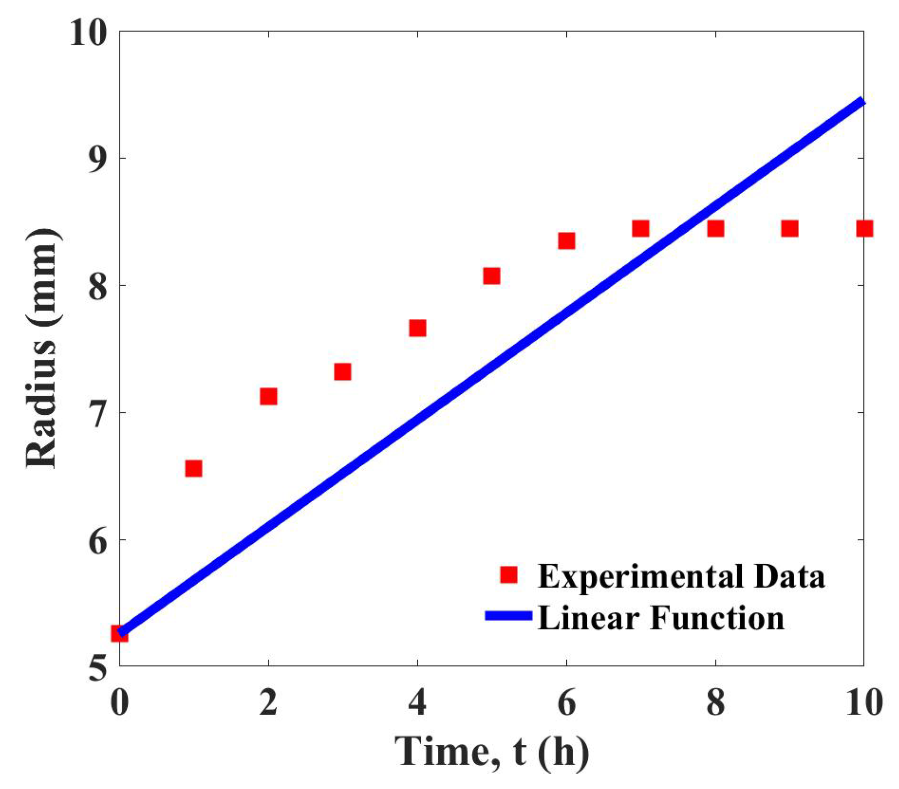
The data of device growth are used to determine the linear function, Equation (3). The curve fitting shown in Figure 2 demonstrates that the linear function gives a satisfactory fit to the experimental data. The determined growth parameter is $g=2.1547\times {10}^{-5}$ with the least squares error, 3.183.

Employing the growth parameter determined above, the fractional drug release data are further fitted to the controlled drug release models; single-phase model, Equation (12), two-phase model, Equation (18), and time-dependent model, Equation (23). The results for all three controlled drug release models are compared.

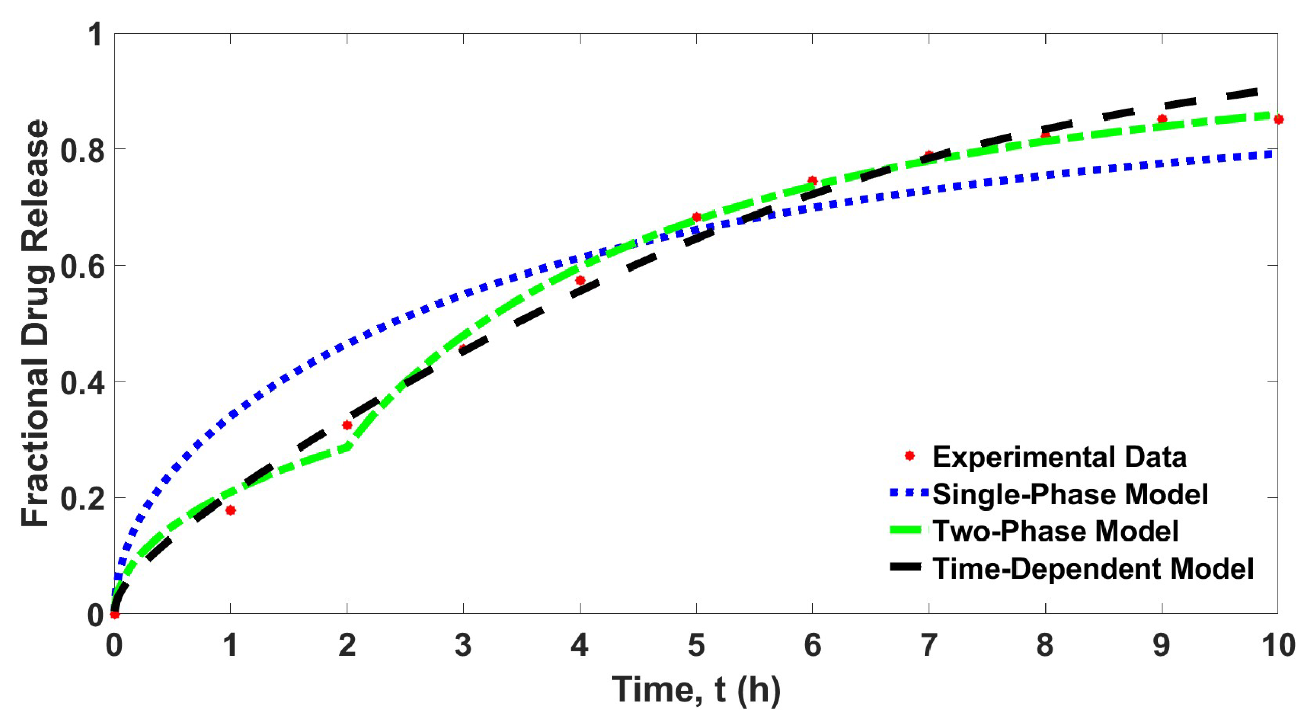
The curve fitting in Figure 3 shows different fitting patterns for all considered controlled drug release models. While the two-phase model and the time-dependent model show a good fit to the experimental data, the single-phase model, however, gives only a satisfactory fit to the experimental data.

Table 1. The determined parameter values and the least squares error for each model.

Models	Single-Phase Model	Two-Phase Model			Time-Dependent Model
	$\mathit{D}$	${\mathit{D}}_{\mathbf{0}}$	${\mathit{D}}_{\mathbf{1}}$	${\mathit{t}}_{\mathit{c}}$	$\mathit{\mu }$
	(mm${}^{\mathbf{2}}/\mathbf{s}$)	(mm${}^{\mathbf{2}}/\mathbf{s}$)	(mm${}^{\mathbf{2}}/\mathbf{s}$)	(s)
Determined Parameter Values	$7.508\times {10}^{-4}$	$2.8535\times {10}^{-4}$	$1.3\times {10}^{-3}$	7200	$6.9722\times {10}^{-8}$
Least-Squares Error	0.0759	0.004			0.0067

shows the determined parameter values for each parameter and the least squares error for each controlled release model.

Table 1 shows that the determined value of $D_0$ is lower than the determined value of $D_1$ of the two-phase model. The critical time, $t_c$, for this model is shown to be equal to two hours. This result correlates with the result in our previous study [11]. The value of $D_1$ is higher in the second phase due to the increasing of pore size during swelling, which facilitates the drug diffusion. The determined value of D of the single-phase model gives a value in between the values of $D_0$ and $D_1$ of the two-phase model. Meanwhile, for the time-dependent model, the diffusion factor, $\mu$, is determined since the linear diffusion function, $D\left(t\right)$, involves the diffusion factor. A series of initial guess values for $D_0$ in Equation (20) is completed first in order to avoid the local optimum. It is found that $D_0=1.549\times {10}^{-4}$ is the most suitable value among the tested values, and only this value is taken to fit to the experimental data.

Table 1 also shows that the single-phase model gives the largest value of least squares error. This result complements the curve fitting shown in Figure 3. The determined least squares errors for the two-phase model and the time-dependent model are improved about tenfold than that of the single-phase model. Similarly, the extracted data for each model presented in

Table 2. The value for fractional drug release at each hour.

Time (h)	Experimental Data	Single-Phase Model	Two-Phase Model	Time-Dependent Model
0	0	0	0	0
1	0.1786	0.3404	0.2099	0.2069
2	0.3247	0.4648	0.2866	0.3367
3	0.4555	0.5497	0.4795	0.4520
4	0.5746	0.6126	0.5969	0.5556
5	0.6835	0.6610	0.6781	0.6462
6	0.7454	0.6990	0.7366	0.7225
7	0.7888	0.7296	0.7802	0.7848
8	0.8216	0.7545	0.8133	0.8345
9	0.8507	0.7754	0.8391	0.8734
10	0.8507	0.7925	0.8594	0.9034

also showed that the determined values of fractional drug release at all times for time-dependent model and two-phase model are much closer to the experimental data compared to the single-phase model. Surprisingly, the least squares error for the two-phase model is lower than the time-dependent model. This result explains that considering the whole process of drug release in two phases is sufficient to demonstrate controlled drug release with a dynamic diffusion parameter. It is shown that the diffusion parameter can be considered as varied constants instead of a time-dependent function.

However, the time-dependent model exhibits a smooth curve that fits the experimental data, while the two-phase model shows a slight jump at $t_c$. Furthermore, according to

Table 3. The CPU time for each model.

	Single-Phase Model	Two-Phase Model	Time-Dependent Model
Time (s)	0.965107	17.175806	0.730085

, the central processing unit (CPU) time for the time-dependent model is the lowest among all tested models. Despite having a slightly higher least squares error compared to the two-phase model, the time-dependent model requires much less computational time. Hence, it can be said that the time-dependent model is the best model, followed by the two-phase model and then the single-phase model, considering the two factors, low determined value of least squares error, and it is much less time consuming.

The Time-Dependent Model in Logarithmic Coordinate

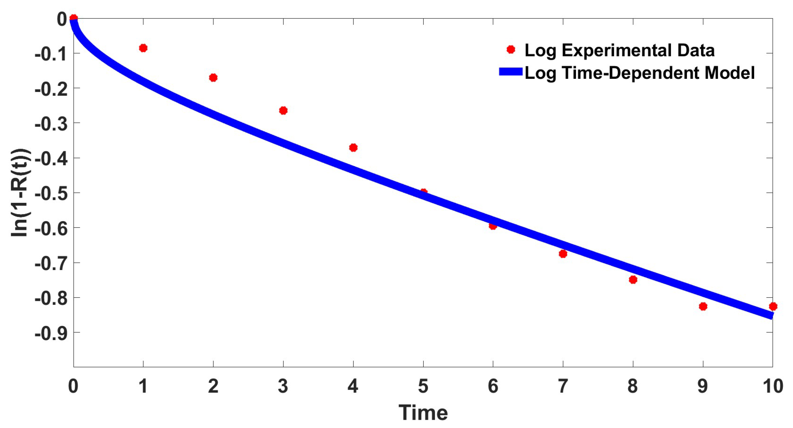
In this subsection, the new time-dependent model is transformed into logarithmic coordinates to further analyse the model. The chosen transformation is written as follows:

$$ln(1-R\left(t\right))=ln\left(\sum _{n=0}^{\infty }\frac{8}{{(2n+1)}^2{\pi }^2.}{e}^{-{\left(\frac{2n+1}{2}\pi \right)}^2.\gamma \left(t\right)}\right).$$

Thus,

$$ln(1-R\left(t\right))=ln\left(\frac{8}{{\pi }^2}\right)+ln\left(\sum _{n=0}^{\infty }\frac{1}{{(2n+1)}^2.}{e}^{-{\left(\frac{2n+1}{2}\pi \right)}^2.\gamma \left(t\right)}\right).$$

(24)

Equation (24) is fitted to the experimental data that had been transformed into the same logarithmic coordinates. The value of the diffusion factor, $\mu$, is determined as $1.3709\times {10}^{-8}$ with the error of $0.0374$. The result of the fitting is presented in Figure 4. The determined parameter in this logarithmic coordinate is comparable to the original fitting presented in Table 1 with slightly higher error.

This numerical test has shown that the proposed time dependent model is able to represent the experimental data even after the chosen transformation. However, unlike most of the previous study, our proposed time-dependent model cannot be written in linear form after the logarithmic transformation [28,29,30]. Hence, it is the best to perform the curve fitting using the original equation for this time dependent model.

4. Conclusions

In this study, three different controlled release models have been successfully analysed, which are the single-phase model, the two-phase model, and the time-dependent model. The single- and two-phase models are previously developed models while the time-dependent model is a newly developed model that assumes the linear growth of device size and linear diffusivity. In the future, the model can be improvised by replacing the linear equations by logistic equations. The controlled drug release models have been developed based on the solution of the advection–diffusion equation governing drug concentration by the Landau transformation method and the separation of variables method. All the developed models have been tested using experimental data under the MATLAB environment. The results show that the two-phase model and the model with time-dependent diffusion give good fittings to the experimental data and have the fitting errors more than 10 times smaller than that from the single-phase model. Although the time-dependent model gives a slightly higher least squares error compared to the two-phase model, it exhibits a smoother fitted curve compared to that from the two-phase model. The CPU time for the time-dependent model is much lower than that for the two-phase model. Therefore, due to its excellent least squares fitting and CPU time efficiency, the new time-dependent model provides the best tool for extracting a diffusion parameter in drug delivery.