Bivariate Poisson 2Sum-Lindley Distributions and the Associated BINAR(1) Processes

Abstract

Discrete-valued time series modeling has witnessed numerous bivariate first-order integer-valued autoregressive process or BINAR(1) processes based on binomial thinning and different innovation distributions. These BINAR(1) processes are mainly focused on over-dispersion. This paper aims to propose new bivariate distributions and processes based on a recently proposed over-dispersed distribution: the Poisson 2S-Lindley distribution. The new bivariate distributions, denoted by the abbreviations BP2S-L(I) and BP2S-L(II), are then used as innovation distributions for the BINAR(1) process. Properties are investigated for both distributions as well as for the BINAR(1) processes. The distribution parameters are estimated using the maximum likelihood method, and the BINAR(1)BP2S-L(I) and BINAR(1)BP2S-L(II) process parameters are estimated using the conditional least squares and conditional maximum likelihood methods. Monte Carlo simulation experiments are conducted to study large and small sample performances and for the comparison of the estimation methods. The Pittsburgh crime series and candy sales datasets are then used to compare the new BINAR(1) processes to some other existing BINAR(1) processes in the literature.

1. Introduction

Count data, or the number of times an event occurs over a set period of time, are becoming ever more abundant in all spheres of human life. In medicine, biology, ecology, economics, demography, and other fields, modeling of these data is becoming pivotal. Real-world situations frequently involve discrete bivariate data that are typically highly related. Some of the examples include counting the number of COVID-19 cases reported in a hospital and the number of deaths among them or counting the number of traffic accidents and the corresponding number of deaths. As a result, bivariate discrete models may be ideal for the statistical analysis of such data.

To this aim, multiple strategies for establishing bivariate random variables have been reported in the literature. Most of them are addressed in [1]. The use of mixed methods to construct discrete and continuous bivariate random variables is often explored in the statistical literature. For instance, see [2,3,4]. The key advantage of this approach is that its marginal probability density function (pdf) or even its moments, correlation, and certain other properties will have simple expressions. A further possibility is to construct it using a new family of distributions. The Sarmanov family of distributions (see [5]) can be used to create bivariate distributions with a variable covariance structure, both discrete and continuous. The authors of [6] looked into several generic approaches to the family formation that took into account different types of marginal distributions. A specific member of the Sarmanov family is the famous Farlie–Gumbel–Morgenstern (FGM) copula.

The expanding number of applications involving time series of counts has necessitated the development of more appropriate integer-valued time series models that can manage the most common phenomena of over-dispersion while also taking into account the cases where two related series are assembled. Since the authors of [7,8] have performed pioneering research on the first-order integer-valued autoregressive (INAR(1)) process with Poisson innovations, plenty of relevant papers with univariate innovation distributions have appeared in the literature. See, for instance,  [9,10,11,12,13]. For the bivariate setting, the authors of [14] introduced the concept of BINAR(1) processes to consider cross-correlations in integer-valued time series models.

On the other hand, a discrete univariate, one-parameter mixture distribution, the Poisson 2Sum-Lindley (P2S-L) distribution, was introduced in [15] by mixing the Poisson distribution with the 2Sum-Lindley (2S-L) distribution (see [16]). A count regression model, as well as an INAR(1) process having the P2S-L distribution, as an innovation distribution is effectively established in [15]. The superior model selection criteria of the P2S-L distribution and the INAR(1)P2S-L process are demonstrated through simulation studies and real-data analysis.

In this paper, we construct two bivariate distributions based on the P2S-L distribution and, motivated by their improved performance; we apply them as innovations to the BINAR(1) process. To be more precise, discrete bivariate distributions based on the P2S-L distribution are framed in this paper using the mixture methodology (the basic bivariate P2S-L, the bivariate Poisson 2S-Lindley I (BP2S-L(I) distribution) as well as the Sarmanov family of distributions (the Sarmanov bivariate P2S-L, bivariate Poisson 2S-Lindley II (BP2S-L(II)) distribution) and both distributions are mounted as innovation distributions in the BINAR(1) process. Hence, the BINAR(1)BP2S-L(I) and BINAR(1)BP2S-L(II) processes are created. Both the processes are then compared with some other recently proposed BINAR(1) processes, as well as those discussed in [14].

We first review the development of the P2S-L distribution and the associated INAR(1) process. Then, bivariate versions are constructed and adapted to the BINAR(1) process with bivariate P2S-L distribution innovations (BP2S-L(I) and BP2S-L(II) distributions) by inducing a cross-correlation between the counting series by assuming the paired P2S-L innovations are jointly distributed.

The remaining parts of the paper are organized as follows: Section 2 reviews the P2S-L distribution and associated INAR(1) process. The construction of the BP2S-L(I) and BP2S-L(II) distributions is discussed in Section 3. Estimation of the unknown parameters and its simulation study are given in Section 4. Both the bivariate distributions are used as innovation distributions for the BINAR(1) process, which is given in Section 5. Estimation of the unknown parameters of the BINAR(1) processes and their simulation is given in Section 6. The empirical importance of the proposed BINAR(1) processes is studied in Section 7. The concluding remarks are given in Section 8.

2. Poisson 2S-Lindley and its Associated INAR(1) Process

The 2S-Lindley (2S-L) distribution was comprehensively defined in [16] as the sum of two independent Lindley random variables (see [17]). Take $Y_1$ and $Y_2$ as two independent random variables with the same parameter $\theta$, and Y as the 2S-L random variable defined by $Y_1+Y_2$. Then, Y has the pdf given by

$$f(y;\theta )=\frac{{\theta }^4}{{(1+\theta )}^2}y\left(\frac{y^2}{6}+y+1\right)e^{-\theta y},y>0,$$

with $\theta >0$. With the same number of parameters (one), the 2S-L distribution has direct stochastic ordering properties with the Lindley distribution, making it a viable alternative. Based on the 2S-L distribution, the authors of [15] recently proposed a discrete distribution by mixing the Poisson and 2S-L distributions, called the Poisson 2S-Lindley (P2S-L) distribution. A random variable X having the P2S-L distribution is characterized by the following stochastic structure:

$$X|\mathsf{\Lambda }=\lambda \sim \mathrm{P}(\lambda ),$$

where $\mathsf{\Lambda }$ is a random variable that follows $2\text{S-L}\left(\theta \right)$, $\theta >0$, $X|\mathsf{\Lambda }=\lambda \sim D$ denotes “conditionally on $\mathsf{\Lambda }=\lambda$, X has the D distribution”, P($\lambda$) denotes the Poisson distribution with parameter $\lambda$, and 2S-L($\theta$) denotes the 2S-L distribution with parameter $\theta$. One can establish that the unconditional probability mass function (pmf) of X is

$$P(x;\theta )=\frac{{\theta }^4(1+x)}{6{(1+\theta )}^{6+x}}\left[x^2+6{(\theta +2)}^2+x(11+6\theta )\right],x=0,1,2,\dots .$$

(1)

Some of the important properties related to moments of X are discussed below:

The probability-generating function (pgf) of X is determined as

$$\begin{array}{c}\hfill \begin{array}{cc}\hfill G\left(s\right)& =\mathrm{E}\left(s^X\right)=\sum _{x=0}^{\infty }{s}^{x}P(x;\theta )=\frac{{\theta }^4{(2-s+\theta )}^2}{{(1+\theta )}^2{(1-s+\theta )}^4},\hfill \end{array}\end{array}$$

(2)

for $\left|s\right|<1+\theta$. The moment-generating function (mgf) of X is derived as

$$M\left(t\right)=\mathrm{E}\left(e^{tX}\right)=\frac{{\theta }^4{\left(2-e^t+\theta \right)}^2}{{(1+\theta )}^2{\left(1-e^t+\theta \right)}^4},$$

for $t\le log(1+\theta )$. From the function above, the mean and variance of X are easily obtained as

$$\mathrm{E}\left(X\right)=\frac{4+2\theta }{\theta +{\theta }^2}$$

(3)

and

$$\mathrm{Var}\left(X\right)=\frac{2\left({\theta }^2+4\theta +2\right)}{{\theta }^2{(1+\theta )}^2},$$

(4)

respectively. In addition, the Fisher index of dispersion (DI) of X is

$$\begin{array}{c}\hfill \begin{array}{cc}\hfill \mathrm{DI}\left(X\right)& =\frac{\mathrm{Var}\left(X\right)}{\mathrm{E}\left(X\right)}=\frac{1}{\theta }+\frac{1}{2+3\theta +{\theta }^2}.\hfill \end{array}\end{array}$$

One can remark that DI(X) can be less than or greater than 1, since $\theta$ is greater than 0. Thus, the P2S-L distribution can have under or over-dispersed properties. However, the study in [15] focuses on the over-dispersed case more deeply. Hence, the P2S-L distribution is effective in using it as an innovation distribution in an INAR(1) process based on binomial thinning, creating the INAR(1)P2S-L process. Such innovation distribution defined the process, its properties, and its effectiveness based on estimation and real data.

3. Construction of the Bivariate Distributions

In  [18], the authors mentioned two methods for the construction of bivariate distributions based on the Poisson-Lindley distribution. That is, one used the basic method of bivariate construction, and the other used the Sarmanov family. In this section, we make use of those two methods for the construction of bivariate distributions: the BP2S-L(I) and BP2S-L(II) distributions.

3.1. The BP2S-L(I) Distribution

Here, a basic method is used for the construction of the BP2S-L(I) distribution.

Definition 1.

Let $\mathit{X}=(X_1,X_2)$ be a bivariate random vector such that

$$\begin{array}{cc}& X_i\mid \mathsf{\Lambda }=\lambda \sim \mathrm{P}\left(\lambda {\varphi }_i\right),i=1,2,X_1\mid \mathsf{\Lambda }and{X}_2\mid \mathsf{\Lambda }independent\hfill \\ \hfill and\\ & \mathsf{\Lambda }\sim 2\text{S-L}\left(\theta \right),\hfill \end{array}$$

with ${\varphi }_i>0$ and $\theta >0$. That is, conditionally on $\mathsf{\Lambda }=\lambda$, the random variables $X_1$ and $X_2$ are independent, and the conditional distribution of $X_i,i=1,2$, is univariate Poisson with parameters $\lambda {\varphi }_i$, denoted by $X_i\mid \mathsf{\Lambda }=\lambda \sim \mathrm{P}\left(\lambda {\varphi }_i\right).$ Then, we can say that $\mathit{X}$ has the BP2S-L(I) distribution. In this case, the unconditional pmf of $\mathit{X}$ is

$$\begin{array}{cc}\hfill P(X_1=x_1,X_2=x_2)& =\frac{{\theta }^4}{6{(\theta +1)}^2}\frac{{\varphi }_1^{x_1}{\varphi }_2^{x_2}\left(x_1+x_2+1\right)!}{x_1!x_2!{\left(\theta +{\varphi }_1+{\varphi }_2\right)}^{x_1+x_2+4}}\times \hfill \\ \hfill & \left\{6{\left(\theta +{\varphi }_1+{\varphi }_2+1\right)}^2+x_1\left[6\left(\theta +{\varphi }_1+{\varphi }_2\right)+2x_2+5\right]\right.\hfill \\ \hfill & \left.+x_2\left[6\left(\theta +{\varphi }_1+{\varphi }_2\right)+5\right]+x_1^2+x_2^2\right\},\hfill \end{array}$$

(5)

where $x_1,x_2=0,1,2,\dots ,{\varphi }_1,{\varphi }_2>0$ and $\theta >0$.

Proof. 

The pmf of the BP2S-L(I) distribution is obtained via the following integral development:

$$\begin{array}{cc}\hfill P\left(X_1=x_1,X_2=x_2\right)& =\underset{0}{\overset{\infty }{\int }}P\left(X_1=x_1,X_2=x_2\mid \mathsf{\Lambda }=\lambda \right)f(\lambda ;\theta )d\lambda \hfill \\ \hfill & =\underset{0}{\overset{\infty }{\int }}\frac{{\left(\lambda {\varphi }_1\right)}^{x_1}{e}^{-\lambda {\varphi }_1}}{x_1!}\frac{{\left(\lambda {\varphi }_2\right)}^{x_2}{e}^{-\lambda {\varphi }_2}}{x_2!}\frac{{\theta }^4}{{(1+\theta )}^2}\lambda \left(\frac{{\lambda }^2}{6}+\lambda +1\right)e^{-\theta \lambda }d\lambda \hfill \\ \hfill & =\frac{{\theta }^4}{6{(\theta +1)}^2}\frac{{\varphi }_1^{x_1}{\varphi }_2^{x_2}\left(x_1+x_2+1\right)!}{x_1!x_2!{\left(\theta +{\varphi }_1+{\varphi }_2\right)}^{x_1+x_2+4}}\times \hfill \\ \hfill & \left\{6{\left(\theta +{\varphi }_1+{\varphi }_2+1\right)}^2+x_1\left[6\left(\theta +{\varphi }_1+{\varphi }_2\right)+2x_2+5\right]\right.\hfill \\ \hfill & \left.+x_2\left[6\left(\theta +{\varphi }_1+{\varphi }_2\right)+5\right]+x_1^2+x_2^2\right\}.\hfill \end{array}$$

The stated pmf is obtained.    □

Now, a bivariate random vector $\mathit{X}=(X_1,X_2)$ having the BP2S-L(I) distribution is denoted as $\mathit{X}\sim$ BP2S-L(I)($\theta ,{\varphi }_1,{\varphi }_2$).

If $X\sim$ BP2S-L(I)($\theta ,{\varphi }_1,{\varphi }_2$), the marginal pmf of $X_i$, $i=1,2$, can be obtained by the usual procedure, and we have

$$P(X_i=x_i)=\frac{{\theta }^4\left(x_i+1\right){\varphi }_i^{x_i}\left[6{\left(\theta +{\varphi }_i+1\right)}^2+x_i\left(6\theta +6{\varphi }_i+5\right)+x_i^2\right]}{6{(\theta +1)}^2{\left(\theta +{\varphi }_i\right)}^{x_i+4}},x_i=0,1,2,\dots .$$

(6)

Now, the conditional pmf of $X_2|X_1=x_1$ with $x_1=0,1,2,\dots$ can be easily derived as

$$\begin{array}{cc}\hfill & P(X_2=x_2|X_1=x_1)=\frac{\left(x_1+x_2+1\right)!{\varphi }_2^{x_2}{\left(\theta +{\varphi }_1\right)}^{x_1+4}}{\left(x_1+1\right)!x_2!{\left(\theta +{\varphi }_1+{\varphi }_2\right)}^{x_1+x_2+4}}\hfill \\ \hfill & \times \frac{6{\left(\theta +{\varphi }_1+{\varphi }_2+1\right)}^2+x_1\left[6\left(\theta +{\varphi }_1+{\varphi }_2\right)+2x_2+5\right]+x_2\left[6\left(\theta +{\varphi }_1+{\varphi }_2\right)+5\right]+x_1^2+x_2^2}{6{\left(\theta +{\varphi }_1+1\right)}^2+x_1\left(6\theta +6{\varphi }_1+5\right)+x_1^2}\hfill \end{array}$$

(7)

for $x_2=0,1,2,\dots$. The pmf of $X_1|X_2=x_2$ can also be derived in a similar manner.

The joint pgf of $\mathit{X}$ is

$$\begin{array}{c}\hfill G(s_1,s_2)=\mathrm{E}\left({\mathrm{s}}_1^{{\mathrm{X}}_1}{\mathrm{s}}_2^{{\mathrm{X}}_2}\right)=\frac{{\theta }^4{\left[\theta +\left(1-s_1\right){\varphi }_1+\left(1-s_2\right){\varphi }_2+1\right]}^2}{{(\theta +1)}^2{\left[\theta +\left(1-s_1\right){\varphi }_1+\left(1-s_2\right){\varphi }_2\right]}^4}.\end{array}$$

(8)

Now, the mean, variance, and covariance of $X_i$, $i=1,2$, are computed as follows:

The mean of $X_i$ is

$$\mathrm{E}\left(X_i\right)=\frac{2(\theta +2){\varphi }_i}{\theta (\theta +1)}.$$

(9)

The moment of order two of $X_i$ is given by

$$\mathrm{E}\left(X_i^2\right)=\frac{2{\varphi }_i\left[(3\theta (\theta +4)+10){\varphi }_i+\theta (\theta +1)(\theta +2)\right]}{{\theta }^2{(\theta +1)}^2}.$$

(10)

Hence, the variance of $X_i$ can be derived as

$$\mathrm{Var}\left(X_i\right)=\frac{2{\varphi }_i\left[(\theta (\theta +4)+2){\varphi }_i+\theta (\theta +1)(\theta +2)\right]}{{\theta }^2{(\theta +1)}^2}$$

(11)

and the covariance of $X_1$ and $X_2$ as

$$\mathrm{Cov}(X_1,X_2)=\frac{2[3\theta (\theta +4)+10]{\varphi }_1{\varphi }_2}{{\theta }^2{(\theta +1)}^2}.$$

(12)

It should be noted that $\mathrm{Cov}(X_1,X_2)$ is always positive, implying that the BP2S-L(I) distribution is only appropriate for modeling bivariate data with positive correlations.

3.2. The BP2S-L(II) Distribution

The second distribution is based on the scheme characterized by the Sarmanov family of distributions. Indeed, in [5], the Sarmanov family of bivariate distributions based on specific density definitions was introduced. Here, we stress discrete bivariate densities based on the Sarmanov approach. Let us first define how the Sarmanov bivariate density can be formed. Let $X_1$ and $X_2$ be two discrete random variables having the supports ${\chi }_1\subseteq \mathbb{R}$ and ${\chi }_2\subseteq \mathbb{R}$, respectively. Further, let us consider two functions, denoted by $q_i\left(x_i\right),i=1,2$, and defined as bounded non-constant functions such that

$$\sum _{x_i\in {\chi }_i}{q}_i\left(x_i\right)P\left(X_i=x_i\right)=0,i=1,2.$$

(13)

Then the joint pmf of $\mathit{X}=(X_1,X_2)$ for the Sarmanov family can be written as

$$P\left(X_1=x_1,X_2=x_2\right)=P\left(X_1=x_1\right)P\left(X_2=x_2\right)\left[1+\omega q_1\left(x_1\right)q_2\left(x_2\right)\right],$$

(14)

where $\omega$ is a real number, and $\omega q_1\left(x_1\right)q_2\left(x_2\right)$ is a measure of the departure of $X_1$ and $X_2$ from independence such that the following condition is satisfied:

$$1+\omega q_1\left(x_1\right)q_2\left(x_2\right)\ge 0,\mathrm{for}\mathrm{all}{x}_1\in {\chi }_1,x_2\in {\chi }_2.$$

(15)

Different choices for the functions $q_i\left(x_i\right)$, $i=1,2$, can give different cases. Here, following the spirit of [6], we use $q_i\left(x_i\right)={\mathrm{e}}^{-x_i}-L_i\left(1\right)$, where $L_i\left(1\right)$ is the value of the Laplace transform of $X_i$ evaluated at $s=1$. We recall that the Laplace transform of $X_i$ is given by

$$L_i\left(s\right)=E\left(e^{-s{X}_i}\right)=\sum _{x_i\in {\chi }_i}{e}^{-s{x}_i}P(X_i=x_i).$$

(16)

The pmf of the Sarmanov-based bivariate P2S-L or BP2S-L(II) distribution having the P2S-L distribution as a marginal distribution is derived below. First, the Laplace transform for the P2S-L distribution is

$$\begin{array}{c}\hfill L\left(s\right)=\frac{{\theta }^4}{{(\theta +1)}^2}\frac{e^{2s}{[1-e^s(2+\theta )]}^2}{{[1-e^s(1+\theta )]}^4}\end{array}$$

(17)

and, at $s=1$,

$$\begin{array}{c}\hfill L\left(1\right)=\frac{{\theta }^4}{{(\theta +1)}^2}\frac{e^2{[1-e(2+\theta )]}^2}{{[1-e(1+\theta )]}^4}.\end{array}$$

(18)

Then the joint pmf associated with a Sarmanov bivariate distribution takes the form

$$\begin{array}{cc}\hfill & P\left(X_1=x_1,X_2=x_2\right)=\hfill \\ \hfill & P\left(X_1=x_1\right)P\left(X_2=x_2\right)\left[1+\omega \left(e^{-x_1}-L_1\left(1\right)\right)\left(e^{-x_2}-L_2\left(1\right)\right)\right].\hfill \end{array}$$

(19)

Definition 2.

The joint pmf of $\mathit{X}=(X_1,X_2)$ having the Sarmanov bivariate distribution with the P2S-L distribution as a marginal distribution is indicated as

$$\begin{array}{cc}\hfill & P(X_1=x_1,X_2=x_2)=\frac{{\theta }_1^4(1+x_1)}{6{(1+{\theta }_1)}^{6+x_1}}\left[x_1^2+6{({\theta }_1+2)}^2+x_1(11+6{\theta }_1)\right]\times \hfill \\ \hfill & \frac{{\theta }_2^4(1+x_2)}{6{(1+{\theta }_2)}^{6+x_2}}\left[x_2^2+6{({\theta }_2+2)}^2+x_2(11+6{\theta }_2)\right]\times \hfill \\ \hfill & \left[1+\omega \left(e^{-x_1}-\frac{{\theta }_1^4}{{({\theta }_1+1)}^2}\frac{e^2{[1-e(2+{\theta }_1)]}^2}{{[1-e(1+{\theta }_1)]}^4}\right)\left(e^{-x_2}-\frac{{\theta }_2^4}{{({\theta }_2+1)}^2}\frac{e^2{[1-e(2+{\theta }_2)]}^2}{{[1-e(1+{\theta }_2)]}^4}\right)\right],\hfill \end{array}$$

(20)

where $x_1,x_2=0,1,2,\dots$, with ${\theta }_1,{\theta }_2>0$ and ω satisfies (15).

The bivariate random vector $\mathit{X}=(X_1,X_2)$, having the joint pmf (20), is hereafter denoted as $\mathit{X}\sim$ BP2S-L(II)(${\theta }_1,{\theta }_2,\omega$). Hence, if $\mathit{X}\sim$ BP2S-L(II)(${\theta }_1,{\theta }_2,\omega$), the mean and variance of $X_i,i=1,2$, are

$$\begin{array}{c}\hfill \mathrm{E}\left(X_i\right)=\frac{2(2+{\theta }_i)}{{\theta }_i(1+{\theta }_i)}\end{array}$$

(21)

and

$$\begin{array}{c}\hfill \mathrm{Var}\left(X_i\right)=\frac{2\left\{{\theta }_i\left({\theta }_i+1\right)\left({\theta }_i+2\right)+\left[{\theta }_i\left({\theta }_i+4\right)+2\right]\right\}}{{\theta }_i^2{\left({\theta }_i+1\right)}^2},\end{array}$$

(22)

respectively. The covariance between $X_1$ and $X_2$ is computed as

$$\mathrm{Cov}(X_1,X_2)=\omega u_1{u}_2,$$

(23)

where $u_i=\mathrm{E}(X_i{e}^{-X_i}-X_i{L}_i\left(1\right))$. More precisely, for the BP2S-L(II) distribution, we get

$$\begin{array}{ccc}\hfill u_i& =& \frac{2e^2{\theta }_i^4(e({\theta }_i+2)-1)(e({\theta }_i+3)-1)}{{({\theta }_i+1)}^2{(e({\theta }_i+1)-1)}^5}-\frac{2({\theta }_i+2)e^2{\theta }_i^4{[e({\theta }_i+2)-1]}^2}{{\theta }_i({\theta }_i+1){({\theta }_i+1)}^2{[e({\theta }_i+1)-1]}^4}\hfill \\ & & =\frac{2(e-1)e^2{\theta }_i^3\left[e({\theta }_i+2)-1\right]\left[e({\theta }_i+1){({\theta }_i+2)}^2-{\theta }_i({\theta }_i+2)-2\right]}{{({\theta }_i+1)}^3{[e({\theta }_i+1)-1]}^5}.\hfill \end{array}$$

(24)

Further, note that the sign of Cov($X_1,X_2$) depends on the sign of $\omega$.

4. Estimation and Simulation of the Bivariate Distributions

In this section, the estimation of the corresponding parameters of the BP2S-L(I) and BP2S-L(II) distributions, as well as some Monte Carlo experiments for the simulation of parameters, are carried out in detail. The method of maximum likelihood (ML) is used for the estimation of parameters. For both distributions, two sets of parameter values for the sample sizes $n=25,50,100,200,400$ and $N=1000$ number of replications are considered.

4.1. Estimation for the BP2S-L(I) Distribution

Suppose that $(x_{1,i},x{}_{2,i}),$$i=1,2,\dots ,n$, are the observations of a n random sample from $\mathit{X}\sim$ BP2S-L(I)($\theta ,{\varphi }_1,{\varphi }_2$). Then the log of the likelihood function satisfies

$$\begin{array}{ccc}\hfill L\left(\mathit{\beta }\right)& =& \sum _{i=1}^n{x}_{1,i}log{\varphi }_1+\sum _{i=1}^n{x}_{2,i}log{\varphi }_2-\sum _{i=1}^n(x_{1,i}+x_{2,i}+4)log(\theta +{\varphi }_1+{\varphi }_2)\hfill \\ \hfill & +& \sum _{i=1}^{n}log[(1+x_{1,i}+x_{2,i})!]+\sum _{i=1}^{n}log\left\{6{\left(\theta +{\varphi }_1+{\varphi }_2+1\right)}^2\right.\hfill \\ \hfill & +& \left.x_{1,i}\left[6\left(\theta +{\varphi }_1+{\varphi }_2\right)+2x_2+5\right]+x_{2,i}\left[6\left(\theta +{\varphi }_1+{\varphi }_2\right)+5\right]+x_{1,i}^2+x_{2,i}^2\right\}\hfill \\ & -& \sum _{i=1}^n[log(x_{1,i}!)]-\sum _{i=1}^n[log(x_{2,i}!)]+4nlog\theta -nlog\left[6{(\theta +1)}^2\right],\hfill \end{array}$$

(25)

where $\mathit{\beta }=(\theta ,{\varphi }_1,{\varphi }_2)$. The ML estimate (MLE) of $\mathit{\beta }$ or, equivalently, the MLEs of $\theta$, ${\varphi }_1$, and ${\varphi }_2$, are obtained by maximizing (25) using numerical methods. Here, the nlminb function in the R software is used (via the optimization PORT routines) to obtain the MLEs of the parameters in the BINAR(1)BP2S-L(I) process.

4.2. Simulation of Parameters of the BP2S-L(I) Distribution

The MLEs of the BP2S-L(I) distribution parameters are analyzed using a simulation study. The following two sets of parameter values are considered: ($\theta =0.1,{\varphi }_1=0.2,{\varphi }_2=0.4$) and ($\theta =1.5,{\varphi }_1=1.2,{\varphi }_2=1.4$). The bias and mean square errors (MSEs) of the MLEs of the parameters are computed, and the results are reported in Table 1.

Table 1. Simulation results for the BP2S-L(I) distribution.

Sample Size (n)	Parameters	$\mathit{\theta }=0.1,{\mathit{\varphi }}_1=0.2,{\mathit{\varphi }}_2=0.4$		$\mathit{\theta }=1.5,{\mathit{\varphi }}_1=1.2,{\mathit{\varphi }}_2=1.4$
		Bias	MSE	Bias	MSE
25	$\theta$	0.0656	0.0075	0.0316	0.0236
	${\varphi }_1$	0.1377	0.0205	0.0189	0.0197
	${\varphi }_2$	0.2968	0.0927	0.0261	0.0126
50	$\theta$	0.0465	0.0063	0.0291	0.0088
	${\varphi }_1$	0.1347	0.0202	0.0174	0.0100
	${\varphi }_2$	0.2917	0.0909	0.0239	0.0074
100	$\theta$	0.0441	0.0038	0.0277	0.0047
	${\varphi }_1$	0.1321	0.0197	0.0135	0.0056
	${\varphi }_2$	0.2884	0.0898	0.0230	0.0043
200	$\theta$	0.0424	0.0033	0.0239	0.0033
	${\varphi }_1$	0.0580	0.0130	0.0123	0.0033
	${\varphi }_2$	0.1784	0.0554	0.0213	0.0027
400	$\theta$	0.0135	0.0031	0.0219	0.0002
	${\varphi }_1$	0.0127	0.0054	0.0067	0.0018
	${\varphi }_2$	0.0750	0.0175	0.0185	0.0019

Table 1 makes it clear that as the sample size increases, bias and MSE corresponding to each parameter decrease.

4.3. Estimation for BP2S-L(II) Distribution

Let $(x_{1,i},x_{2,i}),$$i=1,2,\dots ,n$, be the observations of a n random sample from $\mathit{X}\sim$ BP2S-L(II)(${\theta }_1,{\theta }_2,\omega$). Then the log of the likelihood function is

$$U\left(\lambda \right)=\sum _{i=1}^{n}log\left[P(X_1=x_{1,i},X_2=x_{2,i})\right],$$

(26)

where $\lambda =({\theta }_1,{\theta }_2,\omega )$ and $P(X_1=x_{1,i},X_2=x_{2,i})$ is the pmf of the BP2S-L(II) distribution defined in (20). Then, (26) had to be maximized to find estimates for $\mathit{\lambda }$. Here also, the optimization technique PORT routines into the nlminb function in the R software is used to obtain the MLEs of the parameters in the BINAR(1)BP2S-L(I) process.

4.4. Simulation of Parameters of the BP2S-L(II) Distribution

In this part, the MLEs of the BP2S-L(II) distribution parameters are analyzed using a simulation study. The two following sets of parameter values are used: (${\theta }_1=0.1,{\theta }_2=0.6,$$\omega =-0.3$) and (${\theta }_1=1.7,{\theta }_2=1.1,\omega =0.6$). The bias and MSEs of the estimates of the parameters are computed, and the results are reported in Table 2.

Table 2. Simulation results for the BP2S-L(II) distribution.

Sample Size $\left(\mathit{n}\right)$	Parameters	${\mathit{\theta }}_1=1.7,{\mathit{\theta }}_2=1.1,\mathit{\omega }=0.6$		${\mathit{\theta }}_1=0.9,{\mathit{\theta }}_2=1,\mathit{\omega }=-0.3$
		Bias	MSE	Bias	MSE
25	${\theta }_1$	0.0599	0.0989	0.1890	0.0419
	${\theta }_2$	0.0672	0.0535	0.1181	0.0433
	$\omega$	0.0036	0.0210	0.0039	0.0105
50	${\theta }_1$	0.0519	0.0509	0.1618	0.0417
	${\theta }_2$	0.0520	0.0247	0.1138	0.0233
	$\omega$	0.0031	0.0099	0.0010	0.0078
100	${\theta }_1$	0.0283	0.0257	0.0941	0.0290
	${\theta }_2$	0.0448	0.0129	0.0794	0.0145
	$\omega$	0.0022	0.0041	0.0006	0.0049
200	${\theta }_1$	0.0238	0.0163	0.0855	0.0290
	${\theta }_2$	0.0377	0.0066	0.0714	0.0233
	$\omega$	0.0011	0.0041	0.0006	0.0004
400	${\theta }_1$	0.0148	0.0092	0.0762	0.0143
	${\theta }_2$	0.0344	0.0041	0.0619	0.0142
	$\omega$	0.0002	0.0009	0.0005	0.0002

5. The Bivariate INAR(1) Processes with Paired P2S-L Innovation Distributions

This section deals with the model development of BINAR(1) processes with the BP2S-L(I) and BP2S-L(II) distributions as innovation distributions.

5.1. General Definition

Let ${\mathit{Y}}_t=(Y_{t,1},Y_{t,2})$, $t=1,2,\dots$, define a BINAR(1) process, such that

$$\begin{array}{cc}\hfill & Y_{t,1}=p_1\circ Y_{t-1,1}+{ϵ}_{t,1}\hfill \\ \hfill & Y_{t,2}=p_2\circ Y_{t-1,2}+{ϵ}_{t,2};p_i\in (0,1),i=1,2,\hfill \end{array}$$

(27)

where ∘ in (27) denotes the binomial thinning operator introduced in [19], which is described as

$$p\circ Y_{t-1}=\sum _{j=1}^{Y_{t-1}}{C}_j,$$

where ${\left\{C_j\right\}}_{j\in \mathbb{Z}}$ is a sequence of independent and identically distributed Bernoulli random variables with parameter p. We assume that the innovation vector ${ϵ}_t$ in (27) is $({ϵ}_{t,1},{ϵ}_{t,2})$ and that ${ϵ}_{t,j}$ is independent of $Y_{s,j}$, $j=1,2$ for each t and s, $s<t$. In addition, let the innovation vector be independent of the counting series in thinning operator ∘. Now, we proceed by assuming ${ϵ}_t$ has both of the discussed distributions, and then we develop the corresponding BINAR(1) processes.

5.2. BINAR(1) Process with BP2S-L(I) Innovation Distributions

For the BINAR(1) process discussed in (27), we suppose that the innovation vector satisfies ${ϵ}_t=({ϵ}_{t,1},{ϵ}_{t,2})\sim$ BP2S-L(I)($\theta ,{\varphi }_1,{\varphi }_2$). Then the resulting ${\mathit{Y}}_t=(Y_{t,1},Y_{t,2})$, $t=1,2,\dots$, is a BINAR(1) process with BP2S-L(I) innovation denoted by BINAR(1)BP2S-L(I).

Suppose that the process ${\mathit{Y}}_t=(Y_{t,1},Y_{t,2})$, $t=1,2,\dots$, is a BINAR(1)BP2S-L(I) process. In this case, the mean, variance, and DI of $Y_{t,i}$, $i=1,2$, are given by

$$\mathrm{E}\left(Y_{t,i}\right)=\frac{2(\theta +2){\varphi }_i}{\theta (\theta +1)(1-p_i)},$$

(28)

$$\mathrm{Var}\left(Y_{t,i}\right)=\frac{2\left[\theta (\theta +4)+2\right]{\varphi }_i^2+2\theta (\theta +1)(\theta +2)\left(p_i+1\right){\varphi }_i}{{\theta }^2{(\theta +1)}^2\left(1-p_i^2\right)}$$

(29)

and

$$\mathrm{DI}\left(Y_{t,i}\right)=1+\frac{\left[\theta (\theta +4)+2\right]{\varphi }_i}{\theta (\theta +1)(\theta +2)\left(1+p_i\right)},$$

(30)

respectively. Note that the DI for the BINAR(1)BP2S-L(I) process is over-dispersed marginally, even though the P2S-L distribution shows under and over-dispersion properties. Now, the conditional mean and variance of components of the process are, for $i=1,2$,

$$\mathrm{E}\left(Y_{t,i}\mid Y_{t-1,i}\right)=p_i{Y}_{t-1,i}+\frac{2(\theta +2){\varphi }_i}{\theta (\theta +1)}$$

(31)

and

$$Var\left(Y_{t,i}\mid Y_{t-1,i}\right)=p_i(1-p_i)Y_{t-1,i}+\frac{2{\varphi }_i\left[\theta (\theta +1)(\theta +2)+(\theta (\theta +4)+2){\varphi }_i\right]}{{\theta }^2{(\theta +1)}^2},$$

(32)

respectively. The covariance of $Y_{t,1}$ and $Y_{t,2}$ is

$$\mathrm{Cov}(Y_{t,1},Y_{t,2})=\frac{2(3\theta (\theta +4)+10){\varphi }_1{\varphi }_2}{{\theta }^2{(\theta +1)}^2(1-p_1{p}_2)}.$$

(33)

The conditional joint pmf of the process is given by

$$P({\mathit{Y}}_t={\mathit{y}}_t\mid {\mathit{Y}}_{t-1}={\mathit{y}}_{t-1})=\sum _{k=0}^u\sum _{s=0}^v{z}_1\left(k\right)z_2\left(s\right)P\left({ϵ}_{t,1}=y_{t,1}-k,{ϵ}_{t,2}=y_{t,2}-s\right),$$

(34)

where ${\mathit{y}}_t=(y_{t,1},y_{t,2})$, $u=min(y_{t,1},y_{t-1,1})$, $v=min(y_{t,2},y_{t-1,2})$,

$$\begin{array}{cc}\hfill & z_1\left(k\right)=\left(\genfrac{}{}{0pt}{}{y_{t-1,1}}{k}\right)p_1^k{\left(1-p_1\right)}^{y_{t-1,1}-k},\hfill \\ \hfill & z_2\left(s\right)=\left(\genfrac{}{}{0pt}{}{y_{t-1,2}}{s}\right)p_2^s{\left(1-p_2\right)}^{y_{t-1,2}-s},\hfill \end{array}$$

${\mathit{y}}_t,{\mathit{y}}_{t-1}\ge 0$ and $P\left({ϵ}_{t,1}=y_{t,1}-k,{ϵ}_{t,2}=y_{t,2}-s\right)$ is given by substituting $x_1$ with $y_{t-1,1}-k$ and $x_2$ with $y_{t-1,2}-s$ in (5).

5.3. BINAR(1) Process with BP2S-L(II) Innovation Distributions

Here, we describe the BINAR(1)BP2S-L(II) process. To this aim, based on the BINAR(1) process, we suppose the innovation vector satisfies: ${ϵ}_t=({ϵ}_{t,1},{ϵ}_{t,2})\sim$ BP2S-L(II)(${\theta }_1,{\theta }_2,\omega$). Further, we assume the assumptions made for the construction of the BINAR(1)BP2S-L(I) process hold too. Then, if ${\mathit{Y}}_t=(Y_{t,1},Y_{t,2})$, $t=1,2,\dots$ for $i=1,2,$ the mean, variance and DI of $Y_{t,i}$, $i=1,2$, are obtained as

$$\mathrm{E}\left(Y_{t,i}\right)=\frac{2({\theta }_i+2)}{{\theta }_i({\theta }_i+1)\left(1-p_i\right)},$$

(35)

$$\mathrm{Var}\left(Y_{t,i}\right)=\frac{2{\theta }_i\left[{\theta }_i\left({\theta }_i+4\right)+\left({\theta }_i+1\right)\left({\theta }_i+2\right)p_i+6\right]+4}{{\theta }_i^2{\left({\theta }_i+1\right)}^2\left(1-p_i^2\right)}$$

(36)

and

$$\mathrm{DI}\left(Y_{t,i}\right)=1+\frac{\frac{1}{{\theta }_i+1}-\frac{1}{{\theta }_i+2}+\frac{1}{{\theta }_i}}{1+p_i},$$

(37)

respectively. In particular, based on the DI, we note that the BINAR(1)BP2S-L(II) process is marginally over-dispersed here also. Now, one step ahead gives the conditional expectation and variance of components of the process for $i=1,2$ as

$$\mathrm{E}\left(Y_{t,i}\mid Y_{t-1,i}\right)=p_i{Y}_{t-1,i}+\frac{2({\theta }_i+2)}{{\theta }_i({\theta }_i+1)}$$

(38)

and

$$Var\left(Y_{t,i}\mid Y_{t-1,i}\right)=p_i(1-p_i)Y_{t-1,i}+\frac{2\left\{{\theta }_i\left({\theta }_i+1\right)\left({\theta }_i+2\right)+\left[{\theta }_i\left({\theta }_i+4\right)+2\right]\right\}}{{\theta }_i^2{\left({\theta }_i+1\right)}^2},$$

(39)

respectively. Furthermore, we have

$$Cov\left(Y_{t,1},Y_{t,2}\mid Y_{t-1,1},Y_{t-1,2}\right)=Cov\left({ϵ}_{t,1},{ϵ}_{t,2}\right),$$

(40)

where

$$\begin{array}{cc}\hfill \mathrm{Cov}({ϵ}_{t,1},{ϵ}_{t,2})& =\omega \frac{2(e-1)e^2{\theta }_1^3\left[e({\theta }_1+2)-1\right]\left[e({\theta }_1+1){({\theta }_1+2)}^2-{\theta }_1({\theta }_1+2)-2\right]}{{({\theta }_1+1)}^3{[e({\theta }_1+1)-1]}^5}\hfill \\ \hfill & \times \frac{2(e-1)e^2{\theta }_2^3\left[e({\theta }_2+2)-1\right]\left[e({\theta }_2+1){({\theta }_2+2)}^2-{\theta }_2({\theta }_2+2)-2\right]}{{({\theta }_2+1)}^3{[e({\theta }_2+1)-1]}^5}.\hfill \end{array}$$

The conditional joint pmf of the BINAR(1)BP2S-L(II) process can be determined by using (34), with the exception that $P({ϵ}_{t,1}={ϵ}_1,{ϵ}_{t,2}={ϵ}_2)$ is swapped by (20).

In addition, under the stationary condition $0<p_i<1$ (see [20]), for both of the models, $\mathrm{E}\left(Y_{t,i}\right),Var\left(Y_{t,i}\right)$ for $i=1,2$ and $\mathrm{Cov}(Y_{t,1},Y_{t,2})$ do not depend on t, and $Var\left(Y_{t,i}\right)$ is finite.

6. Estimation and Simulation of Parameters of the BINAR(1) Processes

The estimation of the parameters and hence the simulation procedures of both the BINAR(1) processes discussed above are studied in detail. For the estimation, the methods of conditional maximum likelihood (CML) and conditional least squares (CLS) are applied.

6.1. Estimation and Simulation of the BINAR(1)BP2S-L(I) Process

Suppose that ${\mathit{Y}}_t=(Y_{t,1},Y_{t,2}),t=1,2,\dots ,n$, is a n random sample from the BINAR(1)BP2S-L(I) process, and consider observations of this sample denoted as ${\mathit{Y}}_t=(y_{t,1},y_{t,2}),t=1,2,\dots ,n$. This subsection explains the methods used for the estimation procedure for the parameters of the BINAR(1)BP2S-L(I) process. For this objective, we set $\mathsf{\Theta }=(\theta ,{\varphi }_1,{\varphi }_2,p_1,p_2)$ as the parameter vector.

6.1.1. Method of Conditional Least Squares Estimation

The CLS estimate (CLSE) of $\mathsf{\Theta }$ for the BINAR(1)BP2S-L(I) process is obtained by minimizing the following equations with respect to $\mathsf{\Theta }$: for $i=1,2$,

$$\begin{array}{cc}\hfill H_i& =\sum _{t=2}^n{\left[y_{t,i}-\mathrm{E}\left(Y_{t,i}\mid Y_{t-1,i}=y_{t-1,i}\right)\right]}^2\hfill \\ \hfill & =\sum _{t=2}^n{\left[y_{t,i}-p_i{y}_{t-1,i}-\frac{2(\theta +2){\varphi }_i}{\theta (\theta +1)}\right]}^2.\hfill \end{array}$$

(41)

Here, we used the quasi-Newton approach (BFGS algorithm in particular) available in the optim function of R software for obtaining the CLSE.

6.1.2. Method of Conditional Maximum Likelihood Estimation

The CML estimate(CMLE) of $\mathsf{\Theta }$ for the BINAR(1)BP2S-L(I) process is computed using the conditional log-likelihood function of the BINAR(1)BP2S-L(I) process. The conditional log-likelihood can be obtained by substituting (34) in the following equation:

$$\begin{array}{c}\hfill \ell \left(\mathsf{\Theta }\right)=\sum _{t=2}^{n}log\left[P({\mathit{Y}}_t={\mathit{y}}_t\mid {\mathit{Y}}_{t-1}={\mathit{y}}_{t-1})\right].\end{array}$$

(42)

The CMLE is obtained by maximizing (42) with respect to $\mathsf{\Theta }$. Furthermore, the consistency and asymptotic normality of the random version of the CMLE under standard regularity conditions are demonstrated in [21,22]. Further, the covariance is obtained as the inverse of Hessian (see [23]), and standard errors (SEs) are the square root of diagonal elements of the covariance matrix. Here, the optimization routines in the nlminb function and fdHess function in the R software are used to obtain the CMLE, observed information matrix, and SEs of the estimates of the parameters in the BINAR(1)BP2S-L(I) process.

6.1.3. Simulation Study for BINAR(1)BP2S-L(I) Process

The estimates obtained for the unknown parameters of the BINAR(1)BP2S-L(I) process via the two methods discussed above are assessed through a simulation study. Here, $N=1000$ samples, each of sizes $n=25,50,100,200,400$ are taken for the two following sets of parameter values: ($\theta =0.1,{\varphi }_1=0.2,{\varphi }_2=0.4;p_1=0.2,p_2=0.15$) and ($\theta =1.2,{\varphi }_1=1.5,{\varphi }_2=1.9,p_1=0.8,p_2=0.6$). For each n, bias and MSEs were calculated and are reported in Table 3 and Table 4.

Table 3. Simulation results for the BINAR(1)BP2S-L(I) process for the set of parameter values: $\theta =0.1,{\varphi }_1=0.2,{\varphi }_2=0.4;p_1=0.2,p_2=0.15$.

Sample Size (n)	Parameters	CLS		CML
		Bias	MSE	Bias	MSE
25	$\theta$	0.0506	0.0075	0.0519	0.0068
	${\varphi }_1$	0.0487	0.0123	0.0487	0.0119
	${\varphi }_2$	0.0571	0.0134	0.0569	0.0134
	$p_1$	0.0652	0.0418	0.0365	0.0246
	$p_2$	0.0586	0.0428	0.0161	0.0208
50	$\theta$	0.0416	0.0035	0.0418	0.0035
	${\varphi }_1$	0.0483	0.0061	0.0483	0.0060
	${\varphi }_2$	0.0571	0.0080	0.0568	0.0080
	$p_1$	0.0258	0.0206	0.0171	0.0160
	$p_2$	0.0285	0.0207	0.0129	0.0140
100	$\theta$	0.0415	0.0028	0.0414	0.0026
	${\varphi }_1$	0.0461	0.0044	0.0458	0.0043
	${\varphi }_2$	0.0499	0.0056	0.0498	0.0056
	$p_1$	0.0166	0.0103	0.0154	0.0097
	$p_2$	0.0120	0.0093	0.0083	0.0079
200	$\theta$	0.0405	0.0020	0.0401	0.0018
	${\varphi }_1$	0.0404	0.0033	0.0405	0.0033
	${\varphi }_2$	0.0432	0.0050	0.0431	0.0048
	$p_1$	0.0075	0.0049	0.0074	0.0047
	$p_2$	0.0053	0.0051	0.0046	0.0049
400	$\theta$	0.0398	0.0019	0.0402	0.0018
	${\varphi }_1$	0.0173	0.0028	0.0165	0.0027
	${\varphi }_2$	0.0274	0.0038	0.0274	0.0030
	$p_1$	0.0031	0.0025	0.0032	0.0021
	$p_2$	0.0052	0.0023	0.0051	0.0022

Table 4. Simulation results for the BINAR(1)BP2S-L(I) process for the set of parameter values: $\theta =1.2,{\varphi }_1=1.5,{\varphi }_2=1.9,p_1=0.8,p_2=0.6$.

Sample Size (n)	Parameters	CLS		CML
		Bias	MSE	Bias	MSE
25	$\theta$	0.1347	0.0742	0.1346	0.0723
	${\varphi }_1$	0.1562	0.1744	0.1630	0.2081
	${\varphi }_2$	0.1073	0.1301	0.0687	0.6277
	$p_1$	0.0939	0.0277	0.1311	0.0343
	$p_2$	0.1087	0.0435	0.1295	0.0448
50	$\theta$	0.1152	0.0508	0.1151	0.0507
	${\varphi }_1$	0.1123	0.1086	0.0953	0.1145
	${\varphi }_2$	0.0415	0.0705	0.0631	0.3437
	$p_1$	0.0574	0.0117	0.0718	0.0135
	$p_2$	0.0491	0.0165	0.0609	0.0174
100	$\theta$	0.0861	0.0425	0.0862	0.0432
	${\varphi }_1$	0.0544	0.0491	0.0489	0.0526
	${\varphi }_2$	0.0140	0.0296	0.0572	0.2037
	$p_1$	0.0321	0.0047	0.0396	0.0053
	$p_2$	0.0275	0.0080	0.0333	0.0083
200	$\theta$	0.0449	0.0392	0.0459	0.0391
	${\varphi }_1$	0.0160	0.0178	0.0129	0.0182
	${\varphi }_2$	0.0120	0.0184	0.0525	0.1303
	$p_1$	0.0159	0.0021	0.0196	0.0022
	$p_2$	0.0169	0.0039	0.0196	0.0040
400	$\theta$	0.0082	0.0342	0.0088	0.0231
	${\varphi }_1$	0.0072	0.0070	0.0064	0.0073
	${\varphi }_2$	0.0062	0.0064	0.0460	0.0731
	$p_1$	0.0084	0.0010	0.0103	0.0010
	$p_2$	0.0083	0.0019	0.0097	0.0018

Table 3 and Table 4 show that as the sample size increases, the bias and MSE corresponding to each parameter decrease for both methods. Although the CLS method performs slightly better than the CML method for the second set of parameters, we further proceed with the CML method since the model comparison is effective with it.

6.2. Estimation and Simulation of the BINAR(1)BP2S-L(II) Process

Suppose that ${\mathit{Y}}_t=(Y_{t,1},Y_{t,2}),t=1,2,\dots ,n$, is a n random sample from the BINAR(1)BP2S-L(II) process, and consider observations of this sample denoted as ${\mathit{y}}_t=(y_{t,1},y_{t,2}),t=1,2,\dots ,n$. This subsection explains the methods used for the estimation procedure for the parameters of the BINAR(1)BP2S-L(II) process. We consider ${\mathsf{\Theta }}^{*}=({\theta }_1,{\theta }_2,\omega ,p_1,p_2)$ as the parameter vector.

6.2.1. Method of Conditional Least Squares Estimation

The CLSE of ${\mathsf{\Theta }}^{*}$ for the BINAR(1)BP2S-L(II) process is obtained by minimizing $H_i^{*}$, $i=1,2,3$, with respect to ${\mathsf{\Theta }}^{*}$, where, for $i=1,2$,

$$\begin{array}{cc}\hfill H_i^{*}& =\sum _{t=2}^n{\left[y_{t,i}-E\left(Y_{t,i}\mid Y_{t-1,i}=y_{t-1,i}\right)\right]}^2\hfill \\ \hfill & =\sum _{t=2}^n{\left[y_{t,i}-p_i{y}_{t-1,i}-\frac{2({\theta }_i+2)}{{\theta }_i({\theta }_i+1)}\right]}^2\hfill \end{array}$$

(43)

and

$$\begin{array}{cc}\hfill H_3^{*}& =\sum _{t=2}^n\left\{\left[y_{t,1}-\mathrm{E}\left(Y_{t,1}\mid Y_{t-1,1}=y_{t-1,1}\right)\right]\left[y_{t,2}-\mathrm{E}\left(Y_{t,2}\mid Y_{t-1,2}=y_{t-1,2}\right)\right]\right.\hfill \\ \hfill & {\left.-Cov\left(Y_{t,1},Y_{t,2}\mid Y_{t-1,1}=y_{t-1,1},Y_{t-1,2}=y_{t-1,2}\right)\right\}}^2.\hfill \end{array}$$

(44)

Here also, we used the BFGS algorithm available in the optim function of the R software for obtaining the CLSE.

6.2.2. Method of Conditional Maximum Likelihood Estimation

The CMLE of ${\mathsf{\Theta }}^{*}$ for the BINAR(1)BP2S-L(II) process utilizes the conditional log-likelihood function indicated as

$$\begin{array}{c}\hfill {\ell }^{\prime }(\mathsf{\Theta }*)=\sum _{t=2}^{n}log\left[P({\mathit{Y}}_t={\mathit{y}}_t\mid {\mathit{Y}}_{t-1}={\mathit{y}}_{t-1})\right],\end{array}$$

(45)

where $P({\mathit{Y}}_t={\mathit{y}}_t\mid {\mathit{Y}}_{t-1}={\mathit{y}}_{t-1})$ is obtained via the joint pmf of (${ϵ}_{t,1},{ϵ}_{t,2}$) by (20). The CMLE is obtained by maximizing (45) according to ${\mathsf{\Theta }}^{*}$. Moreover, the consistency and asymptotic normality of the random version of the CMLE under standard regularity conditions can be proven as given by referring to [21,22]. The covariance is obtained as the inverse of the Hessian matrix, and SEs is the square root of diagonal elements of the covariance matrix. Here also, the optimization routines in the nlminb function and the fdHess function in R software is used to obtain the CMLE, observed information matrix, and hence the SEs of estimates of the parameters in the BINAR(1)BP2S-L(II) process.

6.3. Simulation Study for the BINAR(1)BP2S-L(II) Process

The estimates obtained for the unknown parameters of the BINAR(1)BP2S-L(II) process by the CLS and CML methods are assessed through a simulation study. Thus, $N=1000$ samples each of sizes $n=25,50,100,200,400$ are taken for the two following sets of parametric values: (${\theta }_1=0.1,{\theta }_2=0.3,\omega =0.4,p_1=0.2,p_2=0.15$) and (${\theta }_1=0.5,{\theta }_2=0.6,\omega =-0.3,p_1=0.7,p_2=0.3$). For each n, bias and MSEs were calculated and are reported in Table 5 and Table 6.

Table 5. Simulation results for the BINAR(1)BP2S-L(II) process for the set of parameter values: ${\theta }_1=0.1,{\theta }_2=0.3,\omega =0.4,p_1=0.2,p_2=0.15$.

Sample Size (n)	Parameters	CLS		CML
		Bias	MSE	Bias	MSE
25	${\theta }_1$	0.3645	0.1359	0.4542	0.2144
	${\theta }_2$	0.2411	0.0663	0.2609	0.0762
	$\omega$	0.4026	0.1626	0.3909	0.2281
	$p_1$	0.0638	0.0405	0.2008	0.1312
	$p_2$	0.0665	0.0447	0.1841	0.1343
50	${\theta }_1$	0.3634	0.1355	0.4455	0.2054
	${\theta }_2$	0.2393	0.0625	0.2574	0.0737
	$\omega$	0.4021	0.1622	0.3908	0.2072
	$p_1$	0.0357	0.0196	0.1605	0.1138
	$p_2$	0.0308	0.0193	0.1439	0.1117
100	${\theta }_1$	0.3613	0.1333	0.4395	0.1990
	${\theta }_2$	0.2379	0.0618	0.2533	0.0716
	$\omega$	0.4016	0.1618	0.3887	0.1978
	$p_1$	0.0105	0.009	0.1576	0.1138
	$p_2$	0.0142	0.0096	0.1144	0.0923
200	${\theta }_1$	0.3543	0.1328	0.4325	0.1919
	${\theta }_2$	0.2368	0.0590	0.2509	0.0704
	$\omega$	0.4012	0.1616	0.3727	0.1894
	$p_1$	0.0103	0.0050	0.1246	0.1118
	$p_2$	0.0103	0.0051	0.0941	0.0865
400	${\theta }_1$	0.3579	0.1319	0.4277	0.1867
	${\theta }_2$	0.2286	0.0583	0.2466	0.0677
	$\omega$	0.4011	0.1604	0.3657	0.1804
	$p_1$	0.0043	0.0026	0.0775	0.0044
	$p_2$	0.0029	0.0025	0.0698	0.0826

Table 6. Simulation results for the BINAR(1)BP2S-L(II) process for the set of parameter values: ${\theta }_1=0.5,{\theta }_2=0.6,\omega =-0.3,p_1=0.7,p_2=0.3$.

Sample Size (n)	Parameters	CLS		CML
		Bias	MSE	Bias	MSE
25	${\theta }_1$	0.1444	0.046	0.0339	0.0056
	${\theta }_2$	0.1132	0.0397	0.0315	0.0083
	$\omega$	0.3012	0.0903	0.3103	0.1320
	$p_1$	0.0980	0.0324	0.0483	0.0038
	$p_2$	0.07066	0.0439	0.0211	0.0653
50	${\theta }_1$	0.1437	0.0368	0.0318	0.0053
	${\theta }_2$	0.1159	0.0275	0.3070	0.0071
	$\omega$	0.2992	0.0902	0.3056	0.1266
	$p_1$	0.0506	0.0124	0.0398	0.0245
	$p_2$	0.0368	0.0192	0.0168	0.0584
100	${\theta }_1$	0.1262	0.0309	0.0309	0.0052
	${\theta }_2$	0.1061	0.0197	0.0278	0.0067
	$\omega$	0.2992	0.0901	0.3050	0.1122
	$p_1$	0.0279	0.0058	0.0300	0.0185
	$p_2$	0.0229	0.0103	0.0088	0.0434
200	${\theta }_1$	0.1098	0.2989	0.0304	0.0051
	${\theta }_2$	0.1039	0.0171	0.2064	0.0066
	$\omega$	0.2986	0.0897	0.2920	0.1081
	$p_1$	0.0112	0.0027	0.0269	0.1814
	$p_2$	0.0089	0.0048	0.0034	0.0376
400	${\theta }_1$	0.0750	0.0252	0.0276	0.0046
	${\theta }_2$	0.0956	0.0156	0.0127	0.0065
	$\omega$	0.2978	0.0892	0.2917	0.1019
	$p_1$	0.0077	0.0013	0.0070	0.0163
	$p_2$	0.0038	0.0022	0.0020	0.0273

Table 5 and Table 6 make it clear that as the sample size increases, the bias and MSE of each parameter decrease for both methods. Here we proceed with the CML method for further analysis since it is evident that it performs better than the CLS method.

7. Empirical Study

The results of the suggested BINAR(1) processes are presented in this section using two real, over-dispersed time series count datasets.

7.1. Methodology

Model adequacy criteria are used to compare the proposed BINAR(1) processes to some existing BINAR(1) processes. To that end, we compare the BINAR(1)BP2S-L(I) and BINAR(1)BP2S-L(II) processes to the BINAR(1) bivariate Poisson weighted exponential (BINAR(1)BPWE) process, the BINAR(1) Sarmanov Poisson weighted exponential (BINAR(1)SPWE) process by [24], the BINAR(1) bivariate Poisson (BINAR(1)BP) and BINAR(1) bivariate negative binomial (BINAR(1)BNB) processes by [14], and the BINAR(1)Poisson-Lindley (BINAR(1)PL) process by [20]. The BINAR(1)BPWE and BINAR(1)SPWE processes were chosen since the Poisson-weighted exponential distribution is closely related to the Poisson-Lindley distribution, and the rest of the others were chosen since they have the same number of parameters as that of the BINAR(1)BP2S-L(I) and BINAR(1)BP2S-l(II) processes. Further, the P2S-L distribution is introduced as an alternative to the Poisson-Lindley distribution. Hence, the BINAR(1)PL process is particularly chosen. The BINAR(1)BNB process is commonly used to model over-dispersed count datasets. As we focus here on over-dispersion, we use the BINAR(1)BNB process for comparison.

The estimates of the parameters using the CML method (we used CLS estimates as initial values) along with their SEs and confidence intervals (CIs), -Log-Likelihood (-L), Akaike information criterion (AIC), Bayesian information criterion (BIC), and the root MSE (RMSE) of both the series for all the models described above are calculated. The RMSE represents the sum of squared differences between true values and one-step conditional expectations. Further, as the authors of [25] suggested, the standardized Pearson residuals are calculated to check the accuracy of the BINAR(1)BP2S-L(II) process for both datasets. They are calculated with the following formula:

$$e_t=\frac{y_t-\mathrm{E}\left(Y_{t,i}\mid Y_{t-1,i}=y_{t-1,i}\right)}{\sqrt{Var\left(Y_{t,i}\mid Y_{t-1,i}=y_{t-1,i}\right)}},$$

where $\mathrm{E}\left(Y_{t,i}\mid Y_{t-1,i}=y_{t-1,i}\right)$ and $Var\left(Y_{t,i}\mid Y_{t-1,i}=y_{t-1,i}\right)$ are given in (38) and (39), respectively. Note that the fitted model is an adaptable choice if the mean and variance of $e_t$ are closer to 0 and 1, respectively. The residuals’ autocorrelation function (ACF) is then plotted to see if they are uncorrelated, and the cumulative periodograms (cpgrams) of Pearson residuals for both series are plotted to see if the BINAR(1)BP2S-L(II) process is random for both datasets.

7.2. Crime Series Data

The first data we used are the crime series data from the Pittsburgh police agencies in the file PghCarBeat.csv for the monthly period January 1990 to December 2001. The dataset consists of criminal records of drug activities (CDRUGS) and shooting activities (CSHOTS) in the 12th police car beats in Pittsburgh, with a sample size of 144 each, downloaded from the website www.forecastingprinciples.com. The average CDRUGS and CSHOTS data values are 5.1736 and 5.7569, respectively, with corresponding variances of 13.1794 and 14.2412, indicating a clear over-dispersion. The plots of the time series, ACF, partial ACF (PACF) of the CDRUGS and CSHOTS data are given in Figure 1, Figure 2 and Figure 3, respectively.

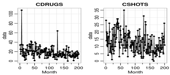
Figure 1. The time-series plot of CDRUGS and CSHOTS data.

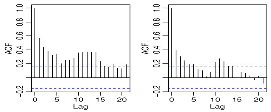
Figure 2. The ACF plot of CDRUGS and CSHOTS data.

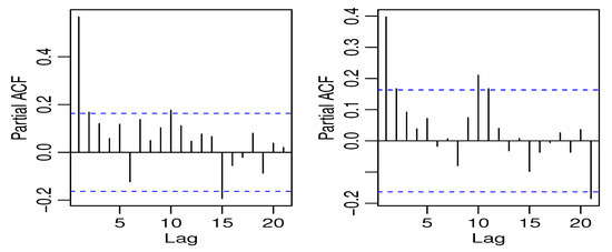
Figure 3. The PACF plot of CDRUGS and CSHOTS data.

The PACF plots make it clear that the data can be used since only the first lag is significant. Further, Figure 4 displays the cross-correlation function (CCF) plot.

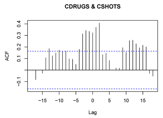
Figure 4. CCF plot of the CDRUGS and CSHOTS datasets.

From Figure 4, we observe that there is a significant cross-correlation in lag 2 between the two time series, which displays positive autocorrelation among both series, which is obvious since after drug use there is a tendency to shoot and vice versa.

Table 7 consists of the CMLEs, AIC, BIC, and RMSEs for the BINAR(1) processes considered here for the crime series dataset.

Table 7. Estimates with SEs and CIs, AIC, BIC, and RMSEs of the considered BINAR(1) processes for the crime series dataset.

Model	Estimates (SEs)	CI	-L	AIC	BIC	RMSEs
BINAR(1)BP2S-L(II)	${\theta }_1=0.9325\left(0.0136\right)$ ${\theta }_2=0.8039\left(0.0116\right)$ $p_1=0.1590\left(1.1905\right)$ $p_2=0.3951\left(0.0322\right)$ $\omega =0.3488 \left(0.0429\right)$	(0.9058, 0.9591) (0.7817, 0.8266) (0, 1) (0.3319, 0.4582) (0.2647, 0.4328)	714.2713	1418.5426	1403.6936	3.0366 3.4383
BINAR(1)BP2S-L(I)	$\theta =0.3672 \left(0.0043\right)$ ${\varphi }_1=0.3425\left(0.0273\right)$ ${\varphi }_2=0.4613\left(0.0118\right)$ $p_1=0.3782\left(0.0290\right)$ $p_2=0.2464\left(0.0413\right)$	(0.3587, 0.3755) (0.2889, 0.3960) (0.4381, 0.4844) (0.3214, 0.4350) (0.1895, 0.3273)	725.8461	1461.6922	1476.5413	3.0477 3.4832
BINAR(1)BPWE	${\mu }_1=2.3271\left(0.2401\right)$ ${\mu }_2=3.4913\left(0.3915\right)$ $p_1=0.4882\left(0.0300\right)$ $p_2=0.3344\left(0.0394\right)$	(1.8565, 2.7976) (2.7239, 4.2586) (0.4294, 0.547) (0.2571, 0.4116)	750.6639	1509.3278	1521.2071	3.0086 3.4742
BINAR(1)SPWE	${\tau }_1=0.3514\left(0.0519\right)$ ${\tau }_2=0.2948\left(0.0315\right)$ $p_1=0.4952\left(0.7971\right)$ $p_2=0.3973\left(0.0311\right)$ $\omega =0.8949 \left(0.0393\right)$	(0.2496, 0.4531) (0.2331, 0.3565) (0, 1) (0.3363, 0.4582) (0.8178, 0.9719)	723.2352	1456.4705	1471.3196	3.0029 3.4515
BINAR(1)BPL	${\lambda }_1=0.5715\left(0.0684\right)$ ${\lambda }_2=0.4644\left(0.0437\right)$ $\varphi =-0.1543 \left(1.0870\right)$ $p_1=0.4126\left(0.0322\right)$ $p_2=0.3488\left(0.0450\right)$	(0.4374, 0.7055) (0.3787, 0.5500) (−2.2848, 1.9762) (0.3495, 0.4757) (0.2606, 0.437)	717.1302	1444.2605	1459.1096	3.0362 3.4575
BINAR(1)BP	${\theta }_1=2.5991\left(0.1707\right)$ ${\theta }_2=3.6519\left(0.2469\right)$ $p_1=0.4703\left(0.0304\right)$ $p_2=0.3598\left(0.0390\right)$ $\omega =0.1461 \left(0.0855\right)$	(2.2645, 2.9336) (3.1679, 4.0458) (0.4107, 0.5298) (0.2833, 0.4362) (0.0696, 0.3139)	766.8106	1543.6212	1558.4703	3.0030 3.4540
BINAR(1)BNB	${\theta }_1=2.5982\left(0.1790\right)$ ${\theta }_2=3.6282\left(0.2714\right)$ $p_1=0.4235\left(0.0242\right)$ $p_2=0.3183\left(0.0309\right)$ $\omega =0.3095 \left(0.0414\right)$	(2.2473, 2.9490) (3.0962, 4.1601) (0.3761, 0.4709) (0, 1) (0.2283, 0.3906)	729.3140	1468.6281	1483.4772	3.0847 3.4751

From Table 7, we observe that the BINAR(1)BP2S-L(II) process performs well for the data because it has the smallest values for the AIC and BIC. The Pearson standardized residuals were calculated for the BINAR(1)BP2S-L(II) process, and we found out that they have the means $-0.046$ and $-0.0261$, and variances $1.060$ and $1.076$, respectively. The ACF plots for standardized residuals for both time series are plotted in Figure 5.

Figure 5. ACF of standardized residuals of CDRUGS and CSHOTS data for the BINAR(1)BP2S-L(II) process.

It clearly indicates that they are uncorrelated, which clearly shows that the BINAR(1)BP2S-L(II) process is accurate and gives a good fit to the crime series dataset. The cpgrams of Pearson residuals of both the series for the crime series dataset are plotted in Figure 6.

Figure 6. Cpgrams of standardized residuals of CDRUGS and CSHOTS data for BINAR(1)BP2S-L(II) process.

From Figure 6, we can infer that the residuals exhibit randomly and without trend distribution.

7.3. Sales Data of Candies

The second dataset is related to some sales data of products on the market. The data are provided by the Kilts Center for Marketing, Graduate School of Business of the University of Chicago. Approximately nine years (1989–1997) of store-level data on the sales of 3500+ UPCs are available in this database (available on the website: http://research.chicagobooth.edu/marketing/databases/dominicks.) Here, we choose two products of candies, which are chewing gum from store ‘56’. The first product, named Candies1, is the ‘CHICLETS TINY PACK’, the UPC of which is ‘1254612128’ and the second product, named Candies2, is the ‘TIC TAC WINTERGREEN’, the UPC of which is ‘980000007’. The sales of these two products from week 1 to week 200 are recorded as the bivariate count time series data. The average Candies1 and Candies2 data values are 18.145 and 12.385, respectively, with corresponding variances of 122.7276 and 45.645, indicating a clear over-dispersion. The plots of the time series, ACF, and PACF of Candies1 and Candies2 data are given in Figure 7, Figure 8, and Figure 9, respectively.

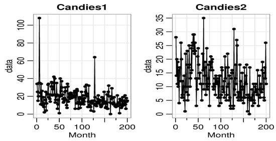
Figure 7. The time series plot of Candies1 and Candies2 data.

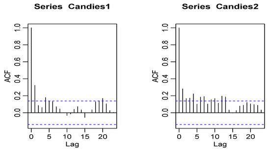
Figure 8. The ACF plot of Candies1 and Candies2 data.

Figure 9. The PACF plot of Candies1 and Candies2 data.

The PACF plots make it clear that the data can be used since only the first lag is significant. Further, Figure 10 displays the CCF plot for candies datasets.

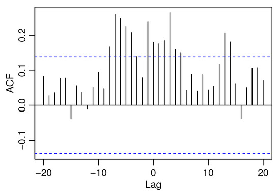
Figure 10. The CCF plot of Candies1 and Candies2 datasets.

The CCF plot shows that the coefficient of lag 0 deviates significantly from 0, which implies the occurrence of cross-correlation. Table 8 consists of the CMLEs, AIC, BIC, and RMSEs for the BINAR(1)s considered here for the sales of candies dataset.

Table 8. Estimates with SEs and CIs, AIC, BIC, and RMSEs of the considered BINAR(1) processes for the sales of candies dataset.

Model	Estimates (SEs)	CI	-L	AIC	BIC	RMSEs
BINAR(1)BP2S-L(II)	${\theta }_1=0.2413\left(0.0141\right)$ ${\theta }_2=0.3546\left(0.0210\right)$ $p_1=0.1914\left(1.9070\right)$ $p_2=0.2027\left(0.0364\right)$ $\omega =0.1266 \left(0.0379\right)$	(0.2136, 0.2690) (0.3133, 0.3959) (0.1201, 0.2628) (0.1284, 0.2771) (0, 1)	1353.2669	2696.5339	2680.0423	10.5923 6.5205
BINAR(1)BP2S-L(I)	$\theta =0.0823 \left(0.0218\right)$ ${\varphi }_1=0.3488\left(0.0460\right)$ ${\varphi }_2=0.2158\left(0.0273\right)$ $p_1=0.1274\left(0.0224\right)$ $p_2=0.1905\left(0.0225\right)$	(0.0395, 0.1251) (0.2587, 0.4390) (0.1622, 0.2694) (0.0833, 0.1714) (0.1465, 0.2346)	1468.821	2947.642	2964.233	10.7085 6.5254
BINAR(1)BPWE	${\mu }_1=12.2172\left(0.9047\right)$ ${\mu }_2=8.7975\left(0.7233\right)$ $p_1=0.2415\left(0.0295\right)$ $p_2=0.2217\left(0.0324\right)$	(10.4438, 13.9906) (7.3798, 10.2152) (0.1836, 0.2995) (0.1581, 0.2852)	1537.859	3083.719	3096.912	10.6145 6.5354
BINAR(1)SPWE	${\tau }_1=0.0879\left(0.0073\right)$ ${\tau }_2=0.1261\left(0.0107\right)$ $p_1=0.3474\left(0.0251\right)$ $p_2=0.3470\left(0.0279\right)$ $\omega =0.999 \left(1.3224\right)$	(0.0735, 0.1023) (0.1049, 0.1472) (0.2982, 0.3965) (0.2923, 0.4018) (0, 1)	0.10227057	2761.133	2744.641	10.4754 6.4828
BINAR(1)BP	${\lambda }_1=13.5602\left(0.4490\right)$ ${\lambda }_2=9.5510\left(0.3888\right)$ $\varphi =2.0940 \left(0.3792\right)$ $p_1=0.2173\left(0.0221\right)$ $p_2=0.1962\left(0.0281\right)$	(12.6801, 14.4404) (8.7888, 10.3131) (1.3508, 2.8373) (0.1741, 0.2606) (0.14139, 0.2511)	1737.278	3484.556	3501.048	10.5450 6.5048
BINAR(1)BNB	${\lambda }_1=12.2871\left(0.6533\right)$ ${\lambda }_2=8.7635\left(0.5255\right)$ $\varphi =0.24366 \left(0.0345\right)$ $p_1=0.2164\left(0.0294\right)$ $p_2=0.1955\left(0.0339\right)$	(11.0066, 13.5677) (7.7334, 9.7935) (0.1760, 0.3113) (0.1587, 0.2743) (0.1289, 0.2621)	1479.710	2969.421	2975.912	11.8279 6.6051
BINAR(1)BPL	${\theta }_1=0.1468\left(0.0096\right)$ ${\theta }_2=0.2109\left(0.0144\right)$ $p_1=0.2877\left(0.02937\right)$ $p_2=0.2948\left(0.03179\right)$ $\omega =0.999 \left(1.5316\right)$	(0.1278, 0.1657) (0.1826, 0.2393) (0.2302, 0.3453) (0.2324, 0.3571) (0, 1)	1359.072	2728.144	2744.636	10.4687 6.4667

From Table 8, we observe that the BINAR(1)BP2S-L(II) process performs well for the data because it has the smallest values for the AIC and BIC. The Pearson standardized residuals were calculated for the BINAR(1)BP2S-L(II) process, and we found out that they have the means $-0.0422$ and $-0.0023$, and variances $1.2940$ and $0.9683$, respectively. The ACF plots for standardized residuals for both time series are plotted in Figure 11.

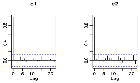
Figure 11. ACF of standardized residuals of Candies1 and Candies2 data for the BINAR(1)BP2S-L(II) process.

It clearly indicates that they are uncorrelated, which clearly shows that the BINAR(1)BP2S-L(II) process is accurate and gives a good fit to the sales of candies dataset. The Pearson residual coefficients of both series for the candies sales dataset are plotted in Figure 12.

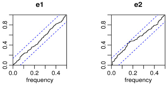
Figure 12. Cpgrams of standardized residuals of Candies1 and Candies2 data for the BINAR(1)BP2S-L(II) process.

From Figure 12, we can also infer that the residuals exhibit randomly and without trend distribution.

8. Concluding Remarks

In this paper, bivariate distributions, namely the BP2S-L(I) and BP2S-L(II) distributions, are constructed based on two different approaches. Both distributions are studied in detail, and the main mathematical properties are derived. The unknown parameters of these distributions were estimated using the ML method. Simulation studies were carried out, and the results show consistent estimates under both distributions. Most importantly, the BINAR(1)BP2S-L(I) and BINAR(1)BP2S-L(II) processes were created with these paired innovation distributions. The unknown parameters of these BINAR(1) processes were estimated by employing the CML and CLS techniques. Both techniques were compared using simulation studies. The crime series and candy sales datasets are then analyzed using these BINAR(1) processes, and the results show that the BINAR(1)BP2S-L(II) process outperforms some other newly proposed BINAR(1) processes in terms of model adequacy metrics. As a result, the BINAR(1) process with various BP2S-L innovation distributions can be regarded as meritorious bivariate time series models that compete with those already published.

References

- Balakrishnan, N.; Lai, C.D. Construction of bivariate distributions. In Continuous Bivariate Distributions; Springer: Berlin/Heidelberg, Germany, 2009; pp. 179–228. [Google Scholar]
- Karlis, D.; Xekalaki, E. Mixed Poisson distributions. Int. Stat. Rev. 2005, 73, 35–58. [Google Scholar] [CrossRef]
- Lai, C.-D. Constructions of discrete bivariate distributions. In Advances in Distribution Theory, Order Statistics, and Inference; Springer: Berlin/Heidelberg, Germany, 2006; pp. 29–58. [Google Scholar]
- Sarabia Alegría, J.M.; Gómez Déniz, E. Construction of multivariate distributions: A review of some recent results. Stat. Oper. Res. Trans. 2008, 32, 3–36. [Google Scholar]
- Sarmanov, O.V. Generalized normal correlation and two-dimensional Fréchet classes. In Doklady Akademii Nauk; Russian Academy of Sciences: Moscow, Russia, 1966; Volume 168, pp. 32–35. [Google Scholar]
- Ting Lee, M.-L. Properties and applications of the Sarmanov family of bivariate distributions. Commun. Stat.-Theory Methods 1996, 25, 1207–1222. [Google Scholar] [CrossRef]
- Al-Osh, M.A.; Alzaid, A.A. First-order integer-valued autoregressive (INAR(1)) process. J. Time Ser. Anal. 1987, 8, 261–275. [Google Scholar] [CrossRef]
- McKenzie, E. Some simple models for discrete variate time series 1. JAWRA J. Am. Water Resour. Assoc. 1985, 21, 645–650. [Google Scholar] [CrossRef]
- Altun, E. A new generalization of geometric distribution with properties and applications. Commun. Stat.-Simul. Comput. 2020, 49, 793–807. [Google Scholar] [CrossRef]
- Altun, E.; Khan, N.M. Modelling with the novel INAR (1)-PTE process. Methodol. Comput. Appl. Probab. 2022, 24, 1735–1751. [Google Scholar] [CrossRef]
- Eliwa, M.S.; Altun, E.; El-Dawoody, M.; El-Morshedy, M. A new three-parameter discrete distribution with associated INAR(1) process and applications. IEEE Access 2020, 8, 91150–91162. [Google Scholar] [CrossRef]
- Irshad, M.R.; Chesneau, C.; D’cruz, V.; Maya, R. Discrete pseudo Lindley distribution: Properties, estimation and application on INAR(1) process. Math. Comput. Appl. 2021, 26, 76. [Google Scholar] [CrossRef]
- Lívio, T.; Khan, N.M.; Bourguignon, M.; Bakouch, H.S. An INAR(1) model with Poisson–Lindley innovations. Econ. Bull. 2018, 38, 1505–1513. [Google Scholar]
- Pedeli, X.; Karlis, D. A bivariate INAR (1) process with application. Stat. Model. 2011, 11, 325–349. [Google Scholar] [CrossRef]
- Chesneau, C.; D’cruz, V.; Maya, R.; Irshad, M.R. A novel discrete distribution based on the mixture of Poisson and sum of two Lindley random variables with regression and an application on INAR(1) process. 2022; Preprint. [Google Scholar]
- Chesneau, C.; Tomy, L.; Gillariose, J. On a sum and difference of two Lindley distributions: Theory and applications. REVSTAT-Stat. J. 2020, 18, 673–696. [Google Scholar]
- Lindley, D. Fiducial distributions and Bayes’ theorem. J. R. Stat. Soc. Ser. B (Methodol.) 1958, 20, 102–107. [Google Scholar] [CrossRef]
- Gomez-Deniz, E.; Sarabia, J.M.; Balakrishnan, N. A multivariate discrete Poisson-Lindley distribution: Extensions and actuarial applications. ASTIN Bull. J. IAA 2012, 42, 655–678. [Google Scholar]
- Steutel, F.; van Harn, K. Discrete analogues of self-decomposability and stability. Ann. Probab. 1979, 7, 893–899. [Google Scholar] [CrossRef]
- Khan, N.M.; Oncel Cekim, H.; Ozel, G. The family of the bivariate integer-valued autoregressive process (BINAR (1)) with Poisson–Lindley (PL) innovations. J. Stat. Comput. Simul. 2020, 90, 624–637. [Google Scholar] [CrossRef]
- Andersen, E.B. Asymptotic properties of conditional maximum-likelihood estimators. J. R. Stat. Soc. Ser. B (Methodol.) 1970, 32, 283–301. [Google Scholar] [CrossRef]
- Bu, R.; McCabe, B. Model selection, estimation and forecasting in INAR (p) models: A likelihood-based Markov chain approach. Int. J. Forecast. 2008, 24, 151–162. [Google Scholar] [CrossRef]
- Freeland, R.K.; McCabe, B.P. Analysis of low count time series data by Poisson autoregression. J. Time Ser. Anal. 2004, 25, 701–722. [Google Scholar] [CrossRef]
- Sajjadnia, Z.; Sharafi, M.; Khan, N.M.; Soobhug, S. The bivariate INAR(1) model with paired Poisson-weighted exponential distributions. 2021; Preprint. [Google Scholar]
- Ristic, M.M.; Popovic, B. A new bivariate binomial time series model. Markov Process. Related Fields 2019, 25, 1–26. [Google Scholar]
Publisher’s Note: MDPI stays neutral with regard to jurisdictional claims in published maps and institutional affiliations. |
© 2022 by the authors. Licensee MDPI, Basel, Switzerland. This article is an open access article distributed under the terms and conditions of the Creative Commons Attribution (CC BY) license (https://creativecommons.org/licenses/by/4.0/).