Development of a Robust Data-Driven Soft Sensor for Multivariate Industrial Processes with Non-Gaussian Noise and Outliers

Abstract

Industrial processes are often nonlinear and multivariate and suffer from non-Gaussian noise and outliers in the process data, which cause significant challenges in data-driven modelling. To address these issues, a robust soft-sensing algorithm that integrates Huber’s M-estimation and adaptive regularisations with multilayer perceptron (MLP) is proposed in this paper. The proposed algorithm, called RAdLASSO-MLP, starts with an initially well-trained MLP for nonlinear data-driven modelling. Subsequently, the residuals of the proposed model are robustified with Huber’s M-estimation to improve the resistance to non-Gaussian noise and outliers. Moreover, a double L1-regularisation mechanism is introduced to minimise redundancies in the input and hidden layers of MLP. In addition, the maximal information coefficient (MIC) index is investigated and used to design the adaptive operator for the L1-regularisation of the input neurons to improve biased estimations with L1-regularisation. Including shrinkage parameters and Huber’s M-estimation parameter, the hyperparameters are determined via grid search and cross-validation. To evaluate the proposed algorithm, simulations were conducted with both an artificial dataset and an industrial dataset from a practical gasoline treatment process. The results indicate that the proposed algorithm is superior in terms of predictive accuracy and robustness to the classic MLP and the regularised soft-sensing approaches LASSO-MLP and dLASSO-MLP.

1. Introduction

Owing to immediacy and low cost, soft sensors are preferred in many practical industrial processes to facilitate intelligent control and optimisation. Compared with mechanism-driven soft sensors, data-driven models based on the measured process data describe the complex processes in a more convenient and efficient manner, and are therefore gaining increasing prevalence in the process industry [1]. There are many machine learning and statistical inference algorithms for data-driven soft sensors, including principal component analysis [2], Gaussian process regression [3], interval fusion with preference aggregation [4], latent structure method [5], and artificial neural networks (ANNs) [6]. Among them, ANNs are capable of modelling nonlinear processes without assigning analytic and specific relationships between the explanatory and response variables. ANNs are imbued with universality to describe complex industrial processes and make it convenient to obtain satisfactory estimations at low cost [7]. Although ANNs are unstable because their initial weights and biases are given randomly, the shortcomings can be avoided through sufficient training and data. There are various ANNs, each with its own advantages and disadvantages, such as the radial-basis-function network [8], recurrent neural network [9,10], extreme learning machine [11], and multilayer perceptron (MLP). As the most commonly used and easy-to-implement ANN, MLP has been proven to be a universal approximator that can fit any function with a three-layer structure. Consequently, MLP has been applied to various regression and classification problems [12,13]. In [14], MLP was trained to describe the nonlinear behaviour of a pH neutralisation process and applied to a model predictive control system for the process. Pham et al. developed a hybrid model with MLP and the intelligent water drop algorithm to improve river streamflow forecasting [15]. To evaluate parallel microchannels, Zoljalali et al. used hybrid MLP to derive models of flow distribution and pressure drop with the change in geometric parameters [16].

In MLP-based soft sensors, redundancies usually exist in the explanatory variables as well as in the hidden layers, which greatly affects the model performance, leading to model degradation and even overfitting. Therefore, the research on input variable selection and structure optimisation of MLP has become an important topic. Variable selection approaches can generally be categorised into the following types: filter-like mutual information (MI) [17], wrapper-like sequential backward selection [18], embedding methods such as the least absolute shrinkage and selection operator (LASSO) [19], the nonnegative garrote (NNG) [20], and other interval fusion-based algorithms [21]. As one of the embedding methods that simultaneously achieves input variable selection and model parameter estimation using sparse regularisations, LASSO was integrated with the L1-regularisation function. Recently, Sun et al. designed LASSO-MLP as the nonlinear extension of the classic LASSO, which enables LASSO to handle highly nonlinear data [19]. Cui and Wang utilised LASSO-MLP with random weights in neural networks to estimate the protein content of milk from its NMR spectrum [22].

For the optimisation of hidden layers of the MLP, structure redundancy can be reduced by pruning the redundant neurons or links. Srivastava et al. designed a dropout method that randomly drops units from the network during the training procedure [23]. Wang et al. developed a global optimisation with NNG to simultaneously shrink the input and hidden weights of MLP [24]. Fan et al. [25] proposed a double L1-regularised MLP (dLASSO-MLP) to prune redundant neurons through a two-stage regularisation approach which has favourable performance and sparsity.

However, LASSO-MLP-based algorithms have two weaknesses that undermine their performance under nonideal industrial operating conditions. First, LASSO is sensitive to non-Gaussian noise because its loss function is based on the ordinary least squares (OLS) technique. Second, actual industrial processes are sometimes unstable and nonideal owing to environmental disturbances, maloperations, and instrumentation deviations. These factors give rise to contaminated and offset samples that significantly undermine the reliability and accuracy of the data-driven soft sensors. Thus, integrating appropriate robust estimation techniques helps to improve robustness. Wang and Leng combined least absolute deviations (LAD) regression with adaptive LASSO to resist the influence of vertical outliers [26]. Owing to their intrinsic mathematical structure, M-estimators exhibit robustness to the non-Gaussian noise and therefore have been widely studied [27]. Various M-estimators have been applied to different robust modelling algorithms, such as the Huber penalty [28], Tukey’s biweight penalty [29], and Hampel’s penalty [30]. Among them, Huber’s M-estimator combines squared loss and absolute loss, which maintains the rate of convergence with small errors while increasing the robustness for large errors. In addition, Huber’s estimator is differentiable everywhere and has such simpler differential coefficients over other M-estimators that the Huber-based iterations of backpropagation in ANNs do not significantly increase the computational complexity.

In addition, LASSO regularisation forces the coefficients of all variables to be equally penalised by continuously tuning the shrinkage hyperparameter, which is somewhat unreasonable. To obtain a more simplified model, it is possible to over-shrink the coefficients of the relevant variables, resulting in biased estimates of the model. In multivariate linear regression models, this issue is adequately addressed by designing adaptive factors onto the regularisation coefficients [31,32]. However, there is little research on the adaptive LASSO regularisation for multivariate nonlinear regression models. This is because, for multivariate nonlinear models, it is difficult to find such indicators that can accurately quantify the importance of each input variable to the output, and then be reasonably mapped as adaptive operators for regularisations.

In this paper, a robust and adaptive version of dLASSO-MLP is proposed to overcome biased estimation and susceptibility to non-Gaussian noise in the measured dataset. Additionally, the proposed algorithm is applied to soft-sensing modelling of the S-Zorb unit. The primary contributions of this study are as follows.

• A robust soft-sensing algorithm that integrates Huber’s M-estimation with double regularised MLP is proposed. The resistance to non-Gaussian noise and outliers in the measured data is substantially improved compared with previous algorithms;
• MIC is used to evaluate the penalty degree of the input variables and design adaptive operators for the L1-regularisation of the input layer of MLP. This adaptive mechanism makes it easier to obtain unbiased model estimates;
• The superiority of the proposed data-driven soft sensor is verified through a normal artificial dataset and its contaminated version with outliers. Then, it is utilised to predict the octane number (RON) of the S-Zorb unit in an actual gasoline treatment process. Compared with state-of-the-art methods, the proposed algorithm exhibits better accuracy and robustness.

The remainder of this paper is organised as follows. Section 2 gives an overview of dLASSO-MLP, MIC, and Huber’s M-estimation. Section 3 presents the methodology underlying the proposed algorithm. Section 4 discusses artificial datasets. Section 5 presents the simulation results of a RON prediction application from an actual industrial process. Section 6 presents concluding remarks.

2. Background Theories

2.1. LASSO Regularisations for MLP

Consider the following linear regression model:

$$y=x\beta +{\beta }_0+\epsilon$$

(1)

where $x=\left[x_1{,x}_2{,\dots ,x}_p\right]$ and y denotes the explanatory and response variables, respectively. Vector $\beta ={\left[{\beta }_1,{\beta }_2,\dots ,{\beta }_p\right]}^T$ is the vector of the magnitude coefficients and $\epsilon$ is the random error. Bias ${\beta }_0$ is assumed to be zero without loss of generality. For the OLS estimation, the general assumption is that random errors $\epsilon$ are normally distributed with variance ${\sigma }^2$ and mean zero. To remove redundant variables, Tibshirani [33] introduced L1-regularisation into OLS estimation by minimising the following loss function:

$$\widehat{\beta } = \mathrm{a}\mathrm{r}\mathrm{g}\mathrm{m}\mathrm{i}\mathrm{n}{\displaystyle \sum }_{\forall \left(x,y\right)\in \left\{X,Y\right\}}{\left(y-x\beta \right)}^2+\lambda {\Vert \beta \Vert }_1$$

(2)

where $\lambda {\Vert \beta \Vert }_1$ is called the LASSO penalty (also the L1-regularisation) and $\lambda$is a nonnegative tuning hyperparameter. With $\lambda$ varying, the L1-regularisation has the capability to shrink some coefficients to be exactly zero. If $\lambda$ is sufficiently large, all magnitude coefficients shrink to zero and a null subset is obtained. If $\lambda$ tends to zero, the LASSO algorithm is equivalent to OLS estimation.

MLP, which is commonly applied to nonlinear problems, performs gradient descent via a backpropagation (BP) algorithm. Figure 1 shows the basic structure of a three-layer MLP, comprising an input layer, a hidden layer, and an output layer. Each layer consists of one or more neurons connected to adjacent neurons, and the number of hidden neurons is usually determined by trial-and-error [34]. Assume that n and p represent the size and dimension of the input dataset, respectively, and that the hidden layer has q neurons. Let $X\in {ℝ}^{n\times p}$ denote the candidate input variables and $y\in {ℝ}^n$ output variables; then, y can be formulated as follows:

$$y={g(W}_O{f(Xw}_H{+b}_H{)+b}_O)$$

(3)

where $w_H=\left[\begin{array}{c}{w}_{11},\cdots ,w_{1q}\\ ⋮ \ddots ⋮\\ w_{p1},\cdots ,w_{\mathrm{pq}}\end{array}\right]$ represents the weight matrix between the input and the hidden layer, and $W_O={\left[W_1{,W}_2,\cdots {,W}_q\right]}^T$ denotes the weight vector between the hidden and output layers. The biases of the hidden and output layers are respectively denoted as $b_H=\left[b_1{,b}_2,\cdots {,b}_q\right]$ and $b_O$. Functions $f\left(·\right)$ and $g\left(·\right)$are activation functions.

To achieve input variable selection for MLP, Sun et al. designed LASSO-MLP [19] by formulating a convex optimisation problem as follows:

$${\widehat{\beta }}_1=\mathrm{a}\mathrm{r}\mathrm{g}\mathrm{m}\mathrm{i}\mathrm{n}{\displaystyle \sum }_{\forall \left(x,y\right)\in \left\{X,Y\right\}}{\left(y-g\left(W_{O}f\left({\beta }_1{xw}_H{+b}_H\right){+b}_O\right)\right)}^2+{\lambda }_1\Vert {\beta }_1{\Vert }_1$$

(4)

where ${\beta }_1$ denotes the shrinkage coefficient of the input neurons and ${\lambda }_1$ denotes the tuning hyperparameter of the input layer. After solving Equation (4), the LASSO-MLP estimation can be calculated using Equation (5):

$$y^{*}=g\left(W_{O}f\left({\widehat{\beta }}_1{xw}_H{+b}_H\right){+b}_O\right)$$

(5)

More advanced than LASSO-MLP, dLASSO-MLP is a two-stage convex optimisation methodology that not only selects input variables, but also optimises hidden layers [25]. Assuming hyperparameter ${\lambda }_2$ and shrinkage coefficient ${\beta }_2$ of hidden layer, then the second stage of dLASSO-MLP is as follows:

$${\widehat{\beta }}_2=\mathrm{a}\mathrm{r}\mathrm{g}\mathrm{m}\mathrm{i}\mathrm{n}{\displaystyle \sum }_{\forall \left(x,y\right)\in \left\{X,Y\right\}}{\left(y-g\left({\beta }_2{W}_{O}f\left({\widehat{\beta }}_1{xw}_H{+b}_H\right){+b}_O\right)\right)}^2+{\lambda }_2\Vert {\beta }_2{\Vert }_1$$

(6)

Correspondingly, the dLASSO-MLP estimation can be calculated using Equation (7):

$$y^{*}=g\left({\widehat{\beta }}_2{W}_{O}f\left({\widehat{\beta }}_1{Xw}_H{+b}_H\right){+b}_O\right)$$

(7)

A schematic of the dLASSO-MLP estimation is shown in Figure 2, where the dashed lines represent inactive weights, and the dashed neurons are neurons removed from the network.

2.2. Maximal Information Coefficient (MIC)

Correlation indexes reflect the closeness of the correlation between variables. They fall within the range [–1, 1], whose magnitudes measure the degree of the importance of corresponding explanatory variables. The Pearson product-moment correlation coefficient is one of the popular correlation indexes and is commonly applied with linearities [35]. To describe nonlinear or mixed models, MIC is a promising tool with universality and equality, which is mainly calculated through the MI and the meshing method [36]. Consider that $I\left(X;Y\right)$ is the MI between the given X and Y, $I\left(X;Y\right)$ can then be expressed as follows:

$$I\left(X;Y\right)={\displaystyle \sum }_{x\in X}{\displaystyle \sum }_{y\in Y}P\left(x,y\right){\mathrm{l}\mathrm{o}\mathrm{g}}_2\frac{P\left(x,y\right)}{p\left(x\right),p\left(y\right)}$$

(8)

where $P\left(x,y\right)$ denotes the joint probability density between X and Y, $p\left(x\right)$ and $p\left(y\right)$ denote the marginal probability density of X and Y, respectively. Then, the different probabilities are obtained according to different meshes, the biggest of which is considered to be MIC, which is expressed as follows:

$$\mathrm{M}\mathrm{I}\mathrm{C}=\mathrm{m}\mathrm{a}\mathrm{x}\left\{\frac{\mathrm{I}\left(X;Y\right)}{{\mathrm{l}\mathrm{o}\mathrm{g}}_2\mathrm{m}\mathrm{i}\mathrm{n}\left\{\left|X\right|,\left|Y\right|\right\}}\right\}$$

(9)

Although MIC is capable of estimating the importance of the explanatory variables to the response variable, it cannot determine the sparsest subset to model the output variable because it lacks a truncation criterion for variable selection. Consequently, MIC is often implemented as an auxiliary technique for other variable selection approaches. In this study, MIC is utilised to evaluate the degree of significance of the explanatory variables to the output variable, and is then designed as an auxiliary factor for the regularisation of the input layer.

2.3. Huber’s M-Estimation

Huber’s M-estimation [37] was designed to adjust different magnitudes of residuals and obtain the robustified estimation, which is formulated as follows:

$$\phi \left(y,y^{*}\right)=\left\{\begin{array}{cc}\frac{1}{2}{\left(y-y^{*}\right)}^2,\hfill & for\left|y-y^{*}\right|\le \gamma \hfill \\ \gamma ·\left(\left|y-y^{*}\right|-\frac{1}{2}\gamma \right),\hfill & \mathrm{o}\mathrm{t}\mathrm{h}\mathrm{e}\mathrm{r}\mathrm{w}\mathrm{i}\mathrm{s}\mathrm{e}\hfill \end{array}\right.$$

(10)

where parameter $\gamma$ determines whether the residual loss is quadratic or linear penalisation. For $\gamma =0$ and $\gamma =\infty$, the Huber loss can be regarded as having two extremes: LAD and OLS. Owing to the inherent robustness of the LAD estimation, Huber’s M-estimation has the capability to deal with deviations caused by outliers. Parameter $\gamma$ is a tuning hyperparameter and is determined through data-driven, trial-and-error approaches.

3. Proposed Methodology

In this section, a robust soft sensor with adaptive double regularisation is proposed. A detailed description of the proposed algorithm is given below.

3.1. Robust dLASSO-MLP with Adaptive Input Variable Selection

In the proposed algorithm, the quadratic residual loss of dLASSO-MLP is replaced with Huber’s M-estimation to make the model estimation more robust to non-Gaussian noise and outliers. Moreover, an adaptive operator is added to the L1-regularisation of input neurons to avoid biased estimates when shrinking the input weights of MLP. The improved dLASSO-MLP is formulated as Equations (11) and (12):

$${\widehat{\beta }}_1=\mathrm{a}\mathrm{r}\mathrm{g}\mathrm{m}\mathrm{i}\mathrm{n}{\displaystyle \sum }_{\forall \left(x,y\right)\in \left\{X,Y\right\}}\phi \left(y, g\left(W_{O}f\left({\beta }_1{xw}_H{+b}_H\right){+b}_O\right)\right)+{\lambda }_1\Vert \delta ⨀{\beta }_1{\Vert }_1$$

(11)

$${\widehat{\beta }}_2=\mathrm{a}\mathrm{r}\mathrm{g}\mathrm{m}\mathrm{i}\mathrm{n}{\displaystyle \sum }_{\forall \left(x,y\right)\in \left\{X,Y\right\}}\phi \left(y, g\left({\beta }_2{W}_{O}f\left({\widehat{\beta }}_1{xw}_H{+b}_H\right){+b}_O\right)\right)+{\lambda }_2\Vert {\beta }_2{\Vert }_1$$

(12)

where $\phi$ is the Huber loss function of Equation (11), $\delta =\left[{\delta }_1,{\delta }_2,\cdots ,{\delta }_p\right]$denotes the adaptive operator (which will be elaborated in the following section), and ⨀ represents the Hadamard product. Because the correlation index of the hidden neurons cannot be obtained, the adaptive regularisation is not included in the hidden layer optimisation of Equation (12).

Such quadratic optimisation problems can be solved using constrained optimisation algorithms. In this study, an active-set algorithm is adopted to obtain the optimal sparse subset [38,39]. The weights between the input and hidden layers of the MLP are updated with the optimal ${\widehat{\beta }}_1$, and then the hidden neurons are updated with ${\widehat{\beta }}_2$. Thus, the predicted value $y^{*}$ of the model can be calculated using Equation (13):

$$y^{*}=g\left({\widehat{\beta }}_2{W}_{O}f\left({\widehat{\beta }}_1{Xw}_H{+b}_H\right){+b}_O\right)$$

(13)

3.2. Design of the Adaptive Operator

For LASSO in Equation (2), to obtain a sparse model, irrelevant variables need to be shrunk to zero. Nevertheless, all input magnitude coefficients share the same hyperparameter ${\lambda }_1$, which means they are shrunk under equal penalty. This is somewhat unfair for significant relevant variables because there is no preferential treatment for their domination. Indiscriminate penalty causes a risk of over-shrinkage of significant relevant variables and a biased estimation of the model.

To address the deficiency of LASSO regularisation, it is necessary to assign the input magnitude coefficients’ different degrees of penalty. We deploy $\delta =\left[{\delta }_1,{\delta }_2,\cdots ,{\delta }_p\right]$ to represent the adaptive penalty vector. To balance the influences, relevant variables should be designated smaller weights and irrelevant variables should be designated larger weights. Under large weights, the magnitude coefficients of irrelevant variables are easier to shrink to zero. This adaptive mechanism of coefficients shrinkage helps to obtain a more unbiased estimation.

Considering that MLP-based approaches are unable to provide specific input weight vectors, it is difficult to obtain a specific benchmark of variable importance. Thus, an appropriate criterion is necessary to measure the correlation between explanatory variables and response variables. By conveniently applying nonlinearities, correlation indexes are promising alternatives. For unbiased shrinkage, the adaptive operator $\delta =\left[{\delta }_1,{\delta }_2,\cdots ,{\delta }_p\right]$ should decrease with the influences of explanatory variables. Then, the relationship between a single pair of ${\delta }_i$ and correlation index ${MIC}_i$ is expressed as follows:

$${\delta }_i=\frac{1}{{MIC}_i}, i=1,2,\dots ,p$$

(14)

In this manner, the adaptive operator forces the coefficients of all input variables to shrink with different penalty strengths. Subsequently, it helps to obtain an unbiased estimation. The superiority of the proposed mechanism was verified through comprehensive comparisons.

3.3. Determination of Hyperparameters

As pivotal factors in the algorithm, the hyperparameters determine the performance of the trained model. Specifically, ${\lambda }_1$ determines the shrinkage degree of the input layer and the size of the dataset, whereas ${\lambda }_2$ determines the simplification degree of the hidden layer. When ${\lambda }_{1lb}$ equals zero and ${\lambda }_{1ub}$ is a sufficiently large value, there must be an optimal ${\lambda }_1\in \left({\lambda }_{1lb},{\lambda }_{1ub}\right)$ such that the selected subset satisfies the optimal combination of input variables. Similarly, hidden neurons are selected and optimised as ${\lambda }_2$ varies within the domain $\left({\lambda }_{2lb},{\lambda }_{2ub}\right)$ to achieve the best performance of the model. Candidate variables and hidden neurons with ${\beta }_{1 \mathrm{or} 2}=0$ are all removed from the MLP. Additionally, the hyperparameter $\gamma$ of Huber’s M-estimation affects the degree of robust estimation. When $\gamma \to 0$, the Huber loss tends toward LAD loss, which tends toward OLS loss when $\gamma \to \infty$. By adjusting the value of $\gamma$, the algorithm can adapt to different degrees of non-Gaussian noise and outliers.

These hyperparameters are determined using a grid search enumeration procedure through cross-validation (CV). Descriptions of the modelling performance criteria and interactive processes implemented in this approach are as follows.

• Model performance criterion: The Bayesian information criterion (BIC) is applied as the evaluation criterion for model selection among a finite model set. BIC was proposed by [36] and adopted as a measure of the trade-off between the model’s accuracy and complexity. It is given as follows:

  $$\mathrm{B}\mathrm{I}\mathrm{C} = {n\mathrm{l}\mathrm{o}\mathrm{g}}_{e}n{\displaystyle \sum }_{\forall y\in Y}{\left(y-y^{*}\right)}^2+\widehat{p}{\mathrm{l}\mathrm{o}\mathrm{g}}_{e}n$$

  (15)

  where n denotes the number of observations and $\widehat{p}$ the number of selected variables.
• Grid search: Compared to experiential adjustments, the grid search method performs hyperparameter tuning exhaustively within the possible hyperparameter combinations. After generating all possible combinations, it is reliable to select the best combination by means of CV. The bound domain of $\gamma$ is [0.01,10], and the bound domain of ${\lambda }_1$ and ${\lambda }_2$ is [${\lambda }_{lb},{\lambda }_{ub}$] in this study, where ${\lambda }_{lb}$ is set as zero and ${\lambda }_{ub}$ is a sufficiently large value that depends on the dimension of the dataset. Subsequently, a list consisting of every possible combination of ${\lambda }_1$, ${\lambda }_2$, and $\gamma$ is generated. The determination of the hyperparameters includes two loops, in which the CV was taken as the inner loop. In the outer loop, each possible combination of hyperparameters was enumerated and performed using a CV procedure.
• Cross-validation: CV is considered one of the simplest and most widely used model-validation approaches. First, the given dataset D is equally divided into K subsets, one of which is considered the validation set, and the others are taken as the training set. Then, the BIC of the current validation set is evaluated using Equation (15). The procedures are repeated K times until each subset is used as the validation set exactly once. Finally, the BIC values are averaged to evaluate the performance of hyperparameter combinations. Combining the above steps, the approach for determining hyperparameter combinations is presented; its pseudocode is outlined in Algorithm 1.

  Algorithm 1. Determination of ${\widehat{\lambda }}_1$and ${\widehat{\lambda }}_2$ via K-fold CV.

  Input: dataset $D=\left\{X,Y\right\}$ Output: the optimal combination of (${\widehat{\lambda }}_1$, ${\widehat{\lambda }}_2$, $\widehat{\gamma }$) Begin algorithm    Generate possible combinations of (${\lambda }_1$, ${\lambda }_2$, $\gamma$) within the parameter space;    Divide the initial dataset $D$ into k disjoint subsets $D_1,D_2,\dots ,D_K$;       for each possible combination          for $k=$ 1: K                  Take $D_k$ as validation set and the others as training set;                  Train an initial MLP with the current training set;                  Integrate robust estimation and adaptive L1-regularisation to the MLP;                  Solve Equations (11) or (12) and get the magnitude coefficient ${\widehat{\beta }}_k$;                  Obtain a new MLP model by replacing ${\beta }_k$ with ${\widehat{\beta }}_k$;                  Calculate ${\mathrm{B}\mathrm{I}\mathrm{C}}_k$ for the current parameter combination through Equation (15);             End for         CV_BIC $=\frac{1}{K}{{\displaystyle \sum }}_{k=1}^K{\mathrm{B}\mathrm{I}\mathrm{C}}_k$;         End for      Return the optimal combination of (${\widehat{\lambda }}_1$, ${\widehat{\lambda }}_2$, $\widehat{\gamma }$) with the minimum CV_BIC.    End algorithm

3.4. Overall Procedure of the Proposed Algorithm

Based on the detailed description of the proposed algorithm in the previous sections, the computation flow of the algorithm can be summarised as presented below, and its flowchart is displayed in Figure 3.

• Calculate the MIC correlation index and adaptive operator using Equations (9) and (14);
• Divide the initial dataset $D=\left\{X,Y\right\}$ into training and testing datasets;
• Implement Algorithm 1 and obtain the optimal hyperparameter combination of (${\widehat{\lambda }}_1$, ${\widehat{\lambda }}_2$, $\widehat{\gamma }$);
• Train a new MLP and obtain the optimal ${\widehat{\beta }}_1$by solving Equation (11) using ${\widehat{\lambda }}_1$ and $\widehat{\gamma }$;
• Update the input weights of the MLP and select the input variables;
• Obtain the optimal ${\widehat{\beta }}_2$ by solving Equation (12) with ${\widehat{\lambda }}_2$ and $\widehat{\gamma }$;
• Optimise the structure of the MLP with ${\widehat{\beta }}_2$;
• Output the simplified dataset and optimised MLP model.

4. Simulations and Results on Artificial Datasets

This section reports the simulation and validation of the proposed algorithm, conducted through an artificial example with normal and contaminated data. Specifically, it is compared with the standard MLP, the embedding data-driven approaches NNG-MLP [20] and LASSO-MLP [19], and the two-stage regularised approach dLASSO-MLP [25].

4.1. Model Evaluation Criteria

The metrics used for the evaluation are as follows:

• Coefficient of determination ($R^2$): This statistic measures the fitness between the predicted $y^{*}$ and the actual observation of y, where $\overline{y}$ is the average of y:

  $$R^2=1-\frac{{{\displaystyle \sum }}_{\forall y,y^{*}\in Y,Y^{*}}{\left(y-y^{*}\right)}^2}{{{\displaystyle \sum }}_{\forall y,y^{*}\in Y,Y^{*}}{\left(y-\overline{y}\right)}^2}$$

  (16)
• Mean square error (MSE): This is the MSE between the predicted $y^{*}$ and measured y, and is formulated as follows:

  $$\mathrm{M}\mathrm{S}\mathrm{E}=\frac{1}{n}{\displaystyle \sum }_{\forall y,y^{*}\in Y,Y^{*}}{\left(y-y^{*}\right)}^2$$

  (17)
• Mean absolute error (MAE): This is the average absolute residual between the predicted $Y^{*}$ and the actual observation of y:

  $$\mathrm{M}\mathrm{A}\mathrm{E}=\frac{1}{n}{\displaystyle \sum }_{\forall y,y^{*}\in Y,Y^{*}}\left|y-y^{*}\right|$$

  (18)

4.2. Experimental Setup

In this study, all algorithms used the same experimental setup. The first 80% of the dataset was used for training and the remainder for testing. All simulations were performed using MATLAB in a Windows 10 environment, with a Ryzen 7 4800H 2.90 GHz CPU and 16 GB RAM. For the respective MLP structures, the hyperbolic tangent function and linear function were chosen as activation functions for the hidden and output layers, respectively. As one of the most classic trust region methods, the Levenberg–Marquardt algorithm was used as the training approach for the BP algorithm with the same initial learning rate. To ensure fairness, the algorithms were initialised with identical MLP structures.

The optimal hyperparameter values of these ANNs were determined via several trials. The number of hidden layers and hidden neurons, the learning rate, and the maximum number of iterations are listed in

Table 1. Hyperparameter values for the MLP used in this study.

Hyperparameter	Value
Hidden layers	1
Hidden neurons	5
Learning rate	0.001
Maximum number of iterations	1000

.

To demonstrate the robustness of the proposed algorithm, a comparative simulation was designed with artificially altered outliers. First, simulations were performed on a normal artificial dataset. Then, the contaminated data were further simulated to demonstrate the robustness of the proposed algorithm. Finally, the proposed algorithm was utilised in the S-Zorb desulphurisation process to predict the RON.

4.3. Simulation Results on Artificial Dataset

4.3.1. Artificial Dataset with Normal Distribution

In this case, an artificial nonlinear function, described in [12], was used to generate the normal dataset with different degrees of redundant variables. The candidate variables $X=\left\{X_1,X_2\right\}$ were divided into related variables $X_1\in {ℝ}^{n\times p_1}$ and irrelevant variables $X_2\in {ℝ}^{n\times p_2}$. $X$ follows a multivariate normal distribution with the covariance of ${\sum }_{i,j}={\rho }^{\left|i-j\right|}$, $\forall i\ne j$, where $\rho$ denotes the collinearity between two different variables. Then, the response variable $Y$ was obtained as follows:

$$y=\left\{\begin{array}{c}\sqrt{X_1·\beta +X_2·0-0.5}+\epsilon , \theta \ge 0.5\\ e^{X_1·\beta +X_2·0+0.5}+\epsilon ,\theta <0.5\end{array}\right.$$

(19)

where $\beta =\left[3, 1.5, 2, 4, 0.5, 1.3, -2.6, -3.5, -5.1, 2\right]$ and $\epsilon$ denotes Gaussian white noise. In this study, $\rho$ was set to 0.8, indicating that there were considerably coupled candidate variables. $p_2$ was respectively set to 10 and 90 to simulate the dataset in low and large dimensions. A total of 1000 observations were generated to build the dataset. Each algorithm was run 10 times; the corresponding average and best performances are presented in

Table 2. Comparison results of different algorithms for normal data ($X_2\in {ℝ}^{n\times 10}$).

Model	${\mathit{R}}^2$		MSE		MAE		Time Cost
	Mean	Best	Mean	Best	Mean	Best
MLP	0.9330	0.9414	0.1206	0.1014	0.2192	0.2084	0.4357
NNG-MLP	0.9460	0.9491	0.0933	0.0880	0.2004	0.1909	5.1777
LASSO-MLP	0.9477	0.9510	0.0904	0.0847	0.1940	0.1819	5.3589
dLASSO-MLP	0.9471	0.9510	0.0929	0.0848	0.2157	0.1969	4.3865
RAdLASSO-MLP	0.9524	0.9548	0.0849	0.0786	0.1926	0.1858	2.6466

and

Table 3. Comparison results of different algorithms for normal data ($X_2\in {ℝ}^{n\times 90}$).

Model	${\mathit{R}}^2$		MSE		MAE		Time Cost
	Mean	Best	Mean	Best	Mean	Best
MLP	0.8732	0.9235	0.1665	0.1310	0.2977	0.2687	0.4405
NNG-MLP	0.9496	0.9528	0.0838	0.0781	0.2171	0.2091	92.9382
LASSO-MLP	0.9508	0.9526	0.0888	0.0788	0.2206	0.2134	40.3202
dLASSO-MLP	0.9523	0.9567	0.0859	0.0760	0.2245	0.2077	19.9748
RAdLASSO-MLP	0.9545	0.9598	0.0799	0.0691	0.2038	0.1888	13.0524

. To validate the effectiveness of the proposed algorithm, the time cost for a single modelling was recorded after all hyperparameters were determined.

In Table 2 and Table 3, the RAdLASSO-MLP has the minimum MSE and maximum $R^2$ among all the algorithms. First, for the artificial dataset with small and large dimensions of irrelevant variables, the embedding variable selection approaches have similar accuracy and perform favourably over the standard MLP. This indicates that the dimension of the input variables influences the prediction performance of MLP. Then, the optimisation of the MLP structure enables the model to generalise better. Notably, in the case of the non-contaminated dataset, the double regularisations with adaptive variable selection improves the predictive performance of the model. In addition, the proposed algorithm has the least training time, demonstrating the superiority of our algorithm in terms of time performance.

4.3.2. Artificial Dataset with Non-Gaussian Noise and Outliers

In the above example, the data were set theoretically and ideally. Notably, it is necessary to validate the robustness of the proposed model through abnormal samples. Abnormal samples can be divided into vertical outliers in response and heavy-tailed points in explanatory variables. In this study, we generated contaminated samples for both response and explanatory variables. Vertical outliers were generated according to the Pauta criterion [40], and were launched with values more than three scaled median absolute deviation (MAD) away from the median of Y, where MAD is expressed as follows [41]:

$$\mathrm{M}\mathrm{A}\mathrm{D}=\mathrm{m}\mathrm{e}\mathrm{d}\mathrm{i}\mathrm{a}\mathrm{n}\left(\left|\mathrm{Y}-\mathrm{m}\mathrm{e}\mathrm{d}\mathrm{i}\mathrm{a}\mathrm{n}\left(\mathrm{Y}\right)\right|\right)$$

(20)

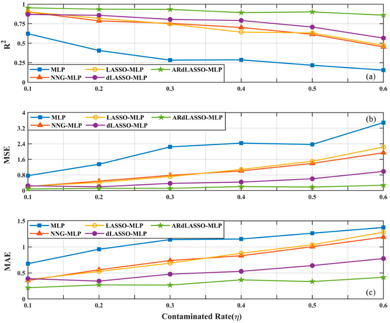
Non-Gaussian noise can be simulated with heavy-tailed points. We generated $\Delta x~N\left(\mu ,1\right)$ with $\mu \ne 0$, randomly selected $x_{ij}\in X$ from the samples, and replaced the original $x_{ij}$ with $x_{ij}+\Delta x$. Let η be the contaminated rate with values of 0.1–0.6. Then, the result with 1000 observations under η = 0.3 is displayed in

Table 4. Comparison results of different algorithms for contaminated data ($\eta$ = 0.3).

Model	${\mathit{R}}^2$		MSE		MAE		Time Cost
	Mean	Best	Mean	Best	Mean	Best
MLP	0.2834	0.3474	2.2393	1.9411	1.1407	1.1041	0.4916
NNG-MLP	0.7543	0.9049	0.7802	0.5192	0.7382	0.6186	53.0698
LASSO-MLP	0.7461	0.8245	0.7176	0.4925	0.6881	0.5893	47.8459
dLASSO-MLP	0.8052	0.9252	0.3685	0.1260	0.4763	0.2666	45.1171
RAdLASSO-MLP	0.9333	0.9495	0.1139	0.0833	0.2669	0.2289	35.1392

, where these algorithms except for RAdLASSO-MLP tend to break down. Further, simulation results under different η are shown in Figure 4, wherein all statistics are compared.

It can be concluded that the RAdLASSO-MLP has a better performance with every statistic, meaning that our algorithm has the best generalisation and resistance to contaminated data. With increases in $\eta$, the superiority of the proposed algorithm becomes more obvious. The $R^2$ of the other four algorithms decrease to under 0.8 when η > 0.3, which demonstrates that the MLPs with MSE as the loss function are sensitive to non-Gaussian noise and outliers. Notably, MLP fails to generalise first and overfit at η = 0.2, whereas the other algorithms maintain a favourable performance. As a basic ANN, MLP has neither the capacity to reduce the model redundancy nor the resistance to outliers. Therefore, under the joint influence of model redundancy and non-Gaussian noise, the overfitting occurred for the MLP. As a result of the robust Huber loss, ARdLASSO-MLP has better prediction accuracy over other algorithms.

5. Application to RON Estimation in S-Zorb Plant

5.1. Overview of the S-Zorb Desulphurisation Plant

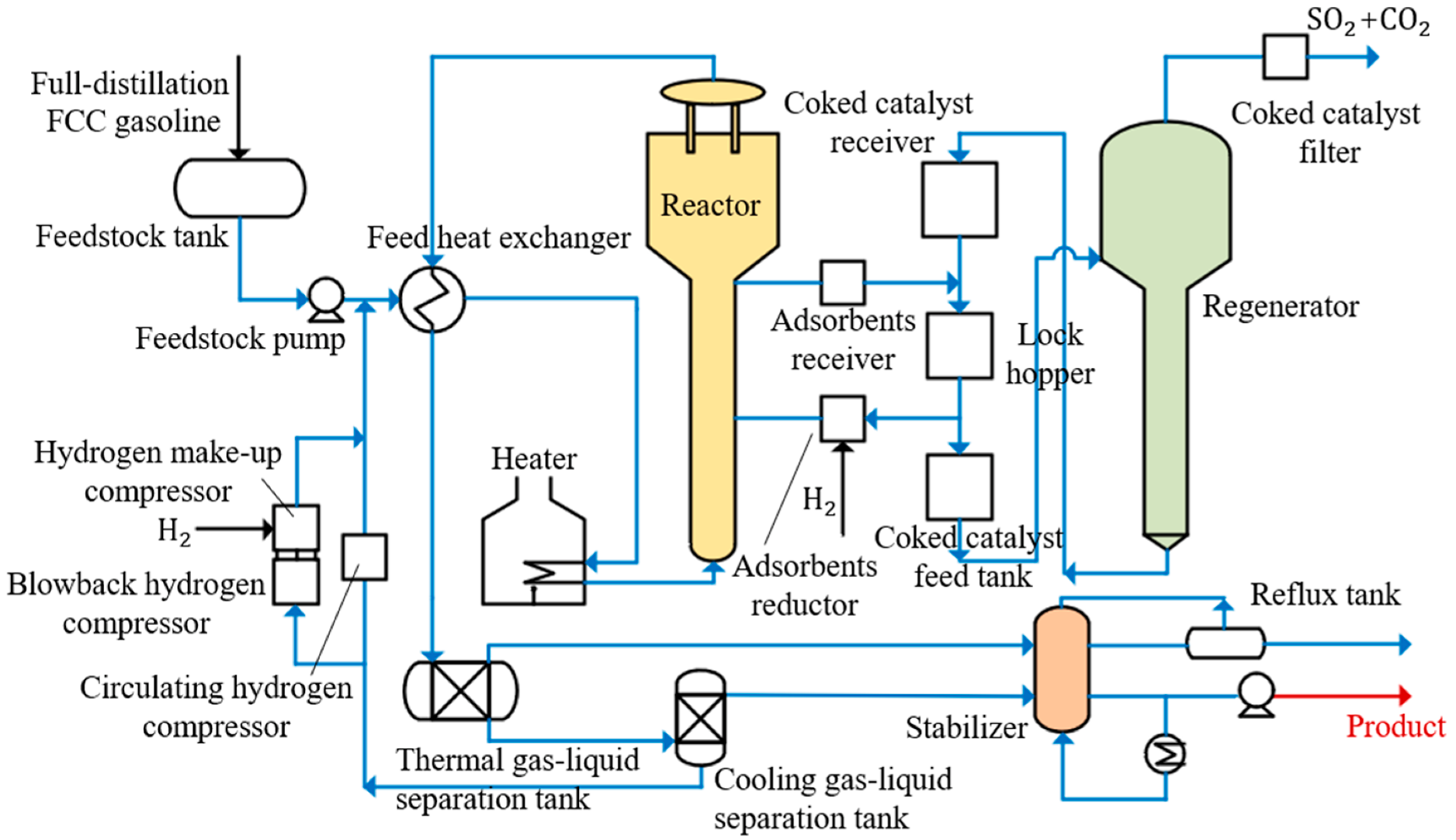
S-Zorb technology, which is based on the principle of reactive adsorption desulphurisation, is generally applied to produce low sulphur and ultra-low sulphur gasoline. The desulphurisation of fluid catalytic cracking (FCC) gasoline is achieved by selective sulphide adsorption and removal. The general scheme of an S-Zorb unit for a gasoline treatment process is shown in Figure 5.

The S-Zorb desulphurisation unit is composed of four main sections: feedstock and desulphurisation, adsorbent regeneration, adsorbent circulation and product stabilisation. With full distillation FCC gasoline as the raw material and reformed hydrogen as the hydrogen source, the adsorption desulphurisation reaction proceeds on the surface of the adsorbents inside the reactor under a given temperature and pressure. The feedstock and desulphurisation system mainly implements adsorption desulphurisation, olefin hydrogenation, and olefin hydroisomerization reactions. The carbon–sulphur bond of the sulphide is broken during the reaction between the sulphur atoms of the sulphide and the adsorbents. Subsequently, the sulphur atoms are removed and adsorbed, after which the hydrocarbon molecules return to the process. Through these chemical reactions, the raw materials are converted into reactive oil and gas, sulphide, and a small amount of coke. Spent adsorbents with sulphur atoms are oxidised and regenerated in the regenerator, and their activity is restored. The regenerated adsorbents are delivered back to the reactor to circulate the regeneration and reaction. Subsequently, the sulphide and coke are burned off during adsorbent regeneration. Additionally, the reactive oil and gas are stabilised to produce low sulphur gasoline, which is clean and stable.

RON is directly determined by the proportion of hydrocarbons in gasoline. A small reduction in RON loss means purer gasoline as well as lower cost. To facilitate the monitoring and analysis of the S-Zorb unit and identify the critical indicators of RON loss, it is necessary to develop an accurate inferential model. However, due to the complicated mechanisms of the S-Zorb unit, mechanism-based models are difficult to implement. In addition, there are numerous operating variables in processes with high nonlinearity and coupling characteristics. Therefore, it is important to develop soft-sensing algorithms with efficient variable selection and model optimisation for the accurate prediction of RON.

The S-Zorb device contained 367 variables, including 354 operating variables, seven feedstock properties, two spent adsorbents, two regenerated adsorbents, and two products. Among these variables, RON was taken as the response variable, whereas the other 365 non-product variables were the explanatory variables. The processing data were collected from a petrochemical plant in China over four years. The S-Zorb desulphurisation is a continuous process and operating variables were sampled every three minutes. Considering the measurement difficulty, the RON was sampled twice a week. It resulted in 325 completely independent processing samples to match the RON measurement.

5.2. Simulations and Discussions

In this study, the first 80% of the data were designated as the training dataset and the remaining data were used for testing. A total of 152 explanatory variables correlated with the response variable over 0.3 were initially selected and considered as candidate input variables, 22 of which were moderately and highly related. After several trials, the initial MLP structure was set to 152–5–1, which means that there were 152 input, five hidden, and one output neuron. To prove the necessity of implementing a robust approach, a determination of whether the measured dataset has outliers has to be made according to the Puata criterion [38]. Figure 6 shows the distribution graph of RON in the measured dataset, in which samples 14, 84, 85, 86, 142, 151, 153, and 189 are identified as outliers.

Table 5. Results of RON estimation with different algorithms.

Model	${\mathit{R}}^2$		MSE		MAE		Time Cost
	Mean	Best	Mean	Best	Mean	Best
MLP	0.0219	0.0236	5.3199	1.9544	1.4170	0.3874	0.5618
NNG-MLP	0.4861	0.8596	0.1496	0.0352	0.2797	0.1538	135.9702
LASSO-MLP	0.6051	0.8866	0.1638	0.0254	0.2257	0.1114	74.3032
dLASSO-MLP	0.8828	0.8753	0.0254	0.0194	0.1196	0.1072	47.2796
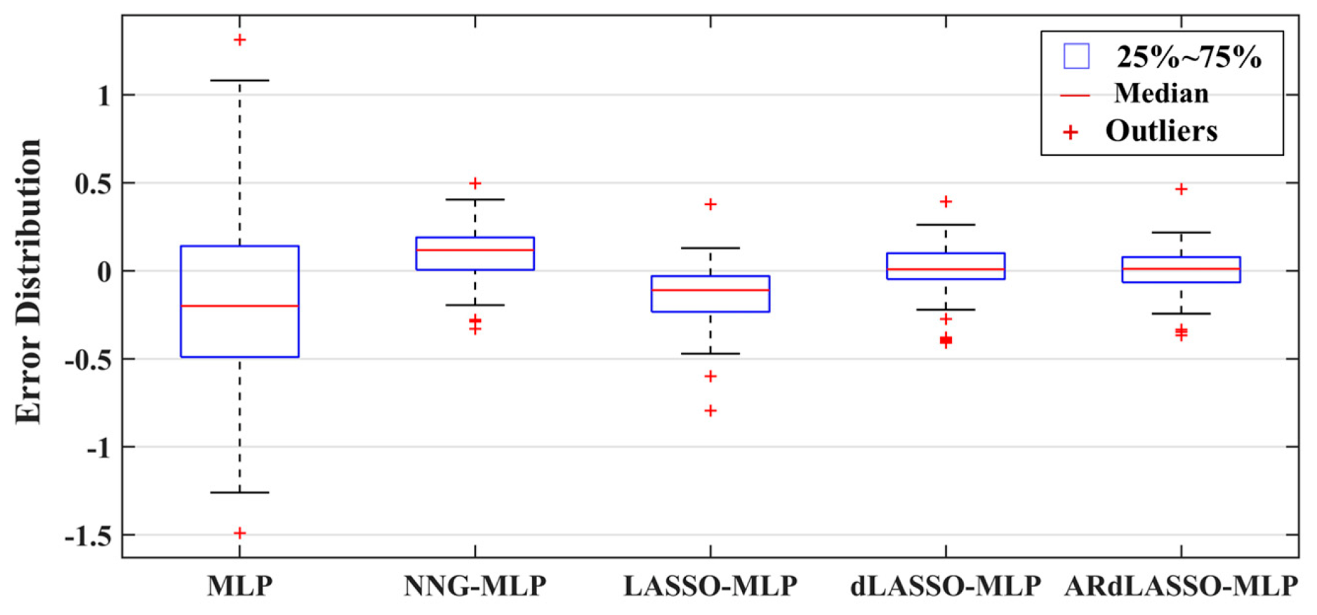
RAdLASSO-MLP	0.9353	0.9465	0.0123	0.0101	0.0789	0.0731	46.0341

shows the mean and the best statistical results for these algorithms over 10 runs. It is clear that the RAdLASSO-MLP outperforms the other algorithms on all criteria. The best regressions and error distributions of these approaches are presented in Figure 7 and Figure 8, where it can be seen that only the RAdLASSO-MLP has $R^2$ over 0.9 and is superior to the other four algorithms. Notably, owing to the insufficiency, nonideality, and redundancy of data, MLP has poorer generalisation with the industrial dataset than that with artificial datasets and has broken to overfitting. It can be concluded that appropriate model reduction and robustified strategies help to obtain more accurate estimations.

6. Conclusions

In this paper, a robust soft-sensing algorithm called RAdLASSO-MLP was proposed for modelling complex industrial processes with outliers and non-Gaussian noise. The proposed algorithm combines the ideologies of the double L1-regularisation algorithm and Huber’s M-estimation to robustly optimise MLP-based soft sensors. In addition, an adaptive mechanism with MIC is designed to discriminately shrink the input weights of the MLP, by which a more unbiased estimation model can be obtained. We demonstrated through simulations that the proposed soft-sensing algorithm performs favourably in terms of robust variable selection and coefficient estimation. RAdLASSO-MLP improves upon dLASSO-MLP in describing nonlinear sparse models with a more unbiased model structure. Furthermore, validating with an artificial example and an actual industrial S-Zorb process, it retained the appealing robust property of Huber’s M-estimation over state-of-the-art soft-sensing approaches.

Although it has been demonstrated that the proposed algorithm is effective for contaminated data and the S-Zorb process in this study, it is not suitable for time-series modelling because of the feedforward structure of MLP. Robust soft-sensing approaches with other recurrent neural networks, such as gated recurrent units or long short-term memory in different industrial scenarios, will be considered in future research.

References

1. Curreri, F.; Patanè, L.; Xibilia, M.G. Soft sensor transferability: A Survey. Appl. Sci. 2021, 11, 7710. [Google Scholar] [CrossRef]
2. Cheng, T.; Harrou, F.; Sun, Y.; Leiknes, T. Monitoring influent measurements at water resource recovery facility using data-driven soft sensor approach. IEEE Sens. J. 2019, 19, 342–352. [Google Scholar] [CrossRef] [Green Version]
3. Zhang, J.; Li, D.; Xia, Y.; Liao, Q. Bayesian aerosol retrieval-based PM2. 5 estimation through hierarchical Gaussian process models. Mathematics 2022, 10, 2878. [Google Scholar] [CrossRef]
4. Muravyov, S.V.; Khudonogova, L.I.; Emelyanova, E.Y. Interval data fusion with preference aggregation. Measurement 2018, 116, 621–630. [Google Scholar] [CrossRef]
5. Lu, B.; Chiang, L. Semi-supervised online soft sensor maintenance experiences in the chemical industry. J. Process Control 2018, 67, 23–34. [Google Scholar] [CrossRef]
6. Song, X.; Han, D.; Sun, J.; Zhang, Z. A data-driven neural network approach to simulate pedestrian movement. Phys. A 2018, 509, 827–844. [Google Scholar] [CrossRef]
7. Abiodun, O.I.; Jantan, A.; Omolara, A.E.; Dada, K.V.; Mohamed, N.A.; Arshad, H. State-of-the-art in artificial neural network applications: A survey. Heliyon 2018, 4, e00938. [Google Scholar] [CrossRef] [Green Version]
8. Montes, F.; Ner, M.; Gernaey, K.V.; Sin, G. Model-based evaluation of a data-driven control strategy: Application to Ibuprofen Crystallization. Processes 2021, 9, 653. [Google Scholar] [CrossRef]
9. Wang, C.C.; Chang, H.T.; Chien, C.H. Hybrid LSTM-ARMA demand-forecasting model based on error compensation for integrated circuit yray manufacturing. Mathematics 2022, 10, 2158. [Google Scholar] [CrossRef]
10. Sun, C.; Zhang, Y.; Huang, G.; Liu, L.; Hao, X. A soft sensor model based on long&short-term memory dual pathways convolutional gated recurrent unit network for predicting cement specific surface area. ISA Trans. 2022. [Google Scholar] [CrossRef]
11. Lama, R.K.; Kim, J.I.; Kwon, G.R. Classification of Alzheimer’s disease based on core-large scale brain network using multilayer extreme learning machine. Mathematics. 2022, 10, 1967. [Google Scholar] [CrossRef]
12. Sun, K.; Sui, L.; Wang, H.; Yu, X.; Jang, S.S. Design of an adaptive nonnegative garrote algorithm for multi-layer perceptron-based soft sensor. IEEE Sens. J. 2021, 21, 21808–21816. [Google Scholar] [CrossRef]
13. Lv, J.; Tang, W.; Hosseinzadeh, H. Developed multiple-layer perceptron neural network based on developed search and rescue optimizer to predict iron ore price volatility: A case study. ISA Trans. 2022. [Google Scholar] [CrossRef]
14. Saki, S.; Fatehi, A. Neural network identification in nonlinear model predictive control for frequent and infrequent operating points using nonlinearity measure. ISA Trans. 2020, 97, 216–229. [Google Scholar] [CrossRef]
15. Pham, Q.B.; Afan, H.A.; Mohammadi, B.; Ahmed, A.N.; Linh, N.T.T.; Vo, N.D.; Moazenzadeh, R.; Yu, P.S. Hybrid model to improve the river streamflow forecasting utilizing multi-layer perceptron-based intelligent water drop optimization algorithm. Soft Comput. 2020, 24, 18039–18056. [Google Scholar] [CrossRef]
16. Zoljalali, M.; Mohsenpour, A.; Amiri, E.O. Developing MLP-ICA and MLP algorithms for investigating flow distribution and pressure drop changes in manifold microchannels. Arab. J. Sci. Eng. 2022, 47, 6477–6488. [Google Scholar] [CrossRef]
17. Min, H.; Ren, W.; Liu, X. Joint mutual information-based input variable selection for multivariate time series modeling. Eng. Appl. Artif. Intell. 2015, 37, 250–257. [Google Scholar]
18. Romero, E.; Sopena, J.M. Performing feature selection with multilayer perceptrons. IEEE Trans. Neural Netw. 2008, 19, 431–441. [Google Scholar] [CrossRef]
19. Sun, K.; Huang, S.H.; Wong, D.S.H.; Jang, S.S. Design and application of a variable selection method for multilayer perceptron neural network with LASSO. IEEE Trans. Neural Netw. Learn. Syst. 2017, 28, 1386–1396. [Google Scholar] [CrossRef]
20. Sun, K.; Liu, J.; Kang, J.L.; Jang, S.S.; Wong, D.S.H.; Chen, D.S. Development of a variable selection method for soft sensor using artificial neural network and nonnegative garrote. J. Process Control 2014, 24, 1068–1075. [Google Scholar] [CrossRef]
21. Muravyov, S.V.; Khudonogova, L.I.; Ho, M.D. Analysis of heteroscedastic measurement data by the self-refining method of interval fusion with preference aggregation—IF&PA. Measurement 2021, 183, 109851. [Google Scholar]
22. Cui, C.H.; Wang, D.H. High dimensional data regression using Lasso model and neural networks with random weights. Inf. Sci. 2016, 372, 505–517. [Google Scholar] [CrossRef]
23. Srivastava, N.; Hinton, G.; Krizhevsky, A.; Sutskever, I.; Salakhutdinov, R. Dropout: A simple way to prevent neural networks from overfitting. J. Mach. Learn. Res. 2014, 15, 1929–1958. [Google Scholar]
24. Wang, H.; Sui, L.; Zhang, M.; Zhang, F.; Ma, F.; Sun, K. A novel input variable selection and structure optimization algorithm for multilayer perceptron-based soft sensors. Math. Probl. Eng. 2021, 2021, 1–10. [Google Scholar] [CrossRef]
25. Fan, Y.; Tao, B.; Zheng, Y. A data-driven soft sensor based on multilayer perceptron neural network with a double LASSO approach. IEEE Trans. Instrum. Meas. 2019, 69, 3972–3979. [Google Scholar] [CrossRef]
26. Wang, H.; Li, G.; Jiang, G. Robust regression shrinkage and consistent variable selection through the LAD-LASSO. J. Bus. Econ. Stat. 2007, 25, 347–355. [Google Scholar] [CrossRef]
27. De Menezes, D.Q.F.; Prata, D.M.; Secchi, A.R.; Pinto, J.C. A review on robust M-estimators for regression analysis. Comput. Chem. Eng. 2021, 147, 107254. [Google Scholar] [CrossRef]
28. Xia, Y.; Wang, J. Robust regression estimation based on low-dimensional recurrent neural networks. IEEE Trans. Neural Netw. Learn. Syst. 2018, 29, 5935–5946. [Google Scholar] [CrossRef]
29. Wang, J.G.; Cai, X.Z.; Yao, Y.; Zhao, C.; Yang, B.H.; Ma, S.W. Statistical process fault isolation using robust nonnegative garrote. J. Taiwan Inst. Chem. Eng. 2020, 107, 24–34. [Google Scholar] [CrossRef]
30. Gijbels, I.; Vrinssen, I. Robust nonnegative garrote variable selection in linear regression. Comput. Stat. Data Anal. 2015, 85, 1–22. [Google Scholar] [CrossRef]
31. Zou, H. The adaptive Lasso and its oracle properties. J. Am. Stat. Assoc. 2012, 101, 1418–1429. [Google Scholar] [CrossRef] [Green Version]
32. Alhamzawi, R.; Ali, H. The Bayesian adaptive lasso regression. Math. Biosci. 2018, 303, 75–82. [Google Scholar] [CrossRef]
33. Tibshirani, R. Regression shrinkage and selection via the Lasso. J. R. Stat. Soc. B 1996, 58, 267–288. [Google Scholar]
34. Lin, Y.J. Explaining critical clearing time with the rules extracted from a multilayer perceptron artificial neural network. Int. J. Electr. Power Energy Syst. 2010, 32, 873–878. [Google Scholar] [CrossRef]
35. Benesty, J.; Chen, J.; Huang, Y.; Cohen, I. Pearson Correlation Coefficient. In Noise Reduction in Speech Processing; Springer Science & Business Media: Berlin/Heidelberg, Germany, 2009; pp. 1–4. [Google Scholar]
36. Schwarz, G. Estimating the dimension of a Model. Ann. Stat. 1978, 6, 461–4646. [Google Scholar] [CrossRef]
37. Huber, P.J. Robust estimation of a location parameter. In Breakthroughs in Statistics; Kotz, S., Johnson, N.L., Eds.; Springer Science & Business Media: New York, NY, USA, 1992; pp. 492–518. [Google Scholar]
38. Ferreau, H.J.; Kirches, C.; Potschka, A.; Bock, H.G. qpOASES: A parametric active-set algorithm for quadratic programming. Math. Program. Comput. 2014, 6, 327–363. [Google Scholar] [CrossRef]
39. Solntsev, S.; Nocedal, J.; Byrd, R. An algorithm for quadratic ℓ1-regularized optimization with a flexible active-set strategy. Optim. Methods Softw. 2015, 30, 1213–1237. [Google Scholar] [CrossRef] [Green Version]
40. Pukelsheim, F. The three Sigma rule. Am. Stat. 1994, 48, 88–91. [Google Scholar]
41. Pham-Gia, T.; Hung, T. The mean and median absolute deviations. Math. Comput. Model. 2001, 34, 921–936. [Google Scholar] [CrossRef]
Figure 1. Structure of a three-layer MLP.
Mathematics 10 03837 g001
Figure 2. Schematic of dLASSO-MLP.
Mathematics 10 03837 g002
Figure 3. Flowchart of the proposed ARdLASSO-MLP.
Mathematics 10 03837 g003
Figure 4. Performance comparison with different η : (a) R 2 ; (b) MSE; (c) MAE.
Mathematics 10 03837 g004
Figure 5. Process graph of an S-Zorb unit.
Mathematics 10 03837 g005
Figure 6. Distribution graph of RON in the measured dataset.
Mathematics 10 03837 g006
Figure 7. Regression between the predicted and measured values with different algorithms: (a) MLP; (b) NNG-MLP; (c) LASSO-MLP; (d) dLASSO-MLP; (e) RAdLASSO-MLP.
Mathematics 10 03837 g007
Figure 8. Error distribution with different algorithms: (a) MLP; (b) NNG-MLP; (c) LASSO-MLP; (d) dLASSO-MLP; (e) RAdLASSO-MLP.
Mathematics 10 03837 g008