A Modified Group Teaching Optimization Algorithm for Solving Constrained Engineering Optimization Problems

Honghua Rao; Heming Jia; Di Wu; Changsheng Wen; Shanglong Li; Qingxin Liu; Laith Abualigah

doi:10.3390/math10203765

,

and

¹

School of Information Engineering, Sanming University, Sanming 365004, China

²

School of Education and Music, Sanming University, Sanming 365004, China

³

School of Computer Science and Technology, Hainan University, Haikou 570228, China

⁴

Hourani Center for Applied Scientific Research, Al-Ahliyya Amman University, Amman 19328, Jordan

Mathematics2022, 10(20), 3765;https://doi.org/10.3390/math10203765

This article belongs to the Special Issue Computational Intelligence: Theory and Applications

Version Notes

Order Reprints

Abstract

The group teaching optimization algorithm (GTOA) is a meta heuristic optimization algorithm simulating the group teaching mechanism. The inspiration of GTOA comes from the group teaching mechanism. Each student will learn the knowledge obtained in the teacher phase, but each student’s autonomy is weak. This paper considers that each student has different learning motivations. Elite students have strong self-learning ability, while ordinary students have general self-learning motivation. To solve this problem, this paper proposes a learning motivation strategy and adds random opposition-based learning and restart strategy to enhance the global performance of the optimization algorithm (MGTOA). In order to verify the optimization effect of MGTOA, 23 standard benchmark functions and 30 test functions of IEEE Evolutionary Computation 2014 (CEC2014) are adopted to verify the performance of the proposed MGTOA. In addition, MGTOA is also applied to six engineering problems for practical testing and achieved good results.

Keywords:

group teaching optimization algorithm; learning motivation strategy; random opposition-based learning; restart strategy; engineering problems

MSC:

49K35

1. Introduction

Meta-heuristic algorithms (MAs) are commonly used to solve global optimization problems. They mainly solve the optimal solution by simulating nature and human intelligence. To a certain extent, they can search globally and find the approximate solution of the optimal solution. The core of MAs is exploration and exploitation. Among them, exploration is to explore the entire search space as much as possible because the optimal solution may exist anywhere in the entire search space. Furthermore, exploitation is to use effective information as much as possible. In most cases, there are specific correlations between the optimal solutions. Use these correlations to adjust gradually, and slowly search from the initial solution to the optimal solution. In general, MAs hope to balance exploration and exploitation as much as possible.

In recent years, many scholars have studied MAs because of their advantages, such as simple operation, intuitive operation, and fast running speed. So far, hundreds of meta-heuristic algorithms have been proposed. According to different design inspirations, MAs can be divided into four categories: swarm-based, evolutionary, physical, and human-based algorithms. The algorithms represented by swarm-based algorithms include Particle Swarm Optimization (PSO) [1], Ant Lion Optimizer (ALO) [2], Bat Algorithm (BA) [3], Slap Swarm Algorithm (SSA) [4], Ant Colony Optimization (ACO) [5], Artificial Bee Colony (ABC) [6], Gray Wolf Optimization (GWO) [7], Krill Herd (KH) [8], Whale Optimization Algorithm (WOA) [9], and Remora Optimization Algorithm (ROA) [10]. Evolutionary algorithms are represented by Genetic Algorithm (GA) [11], Evolution Strategy (ES) [12], Genetic Programming (GP) [13], Biogeography-Based Optimizer (BBO) [14], Evolutionary Programming (EP) [15], Differential Evolution (DE) [16], and Virulence Optimization Algorithm (VOA) [17]. Physical-based algorithms are represented by Simulated Annealing (SA) [18], Gravitational Search Algorithm (GSA) [19], Black Hole Algorithm (BH) [20], Multi-Verse Optimization (MVO) [21], Ray Optimization (RO) [22], and Thermal Exchange Optimization (TEO) [23]. Human-based algorithms are represented by Harmony Search (HS) [24], Teaching Learning-Based Optimization (TLBO) [25], Social Group Optimization (SGO) [26], and Exchanged Market Algorithm (EMA) [27]. These algorithms have a good optimization effect on MAs.

Group Teaching Optimization Algorithm (GTOA) is an MA that was proposed in 2020 [28] and inspired by the group teaching mechanism. GTOA divides students into elite students and ordinary students for group teaching. For different students, teachers have different teaching methods. However, each student is close to the teacher in essence, so the algorithm has better exploitation ability. Each student will consolidate the contents of the teacher’s teaching during the break. However, this way does not fully reflect the idea of group teaching. Therefore, Zhang et al. proposed a group teaching optimization algorithm with information sharing (ISGTOA) to distinguish the learning styles of different groups. ISGTOA has established two teaching methods for elite and ordinary students. The two groups of students can fully communicate through these two methods. This method increases the communication between groups, improves the dependence of students, and makes the algorithm converge faster [29]. However, ISGTOA still does not distinguish between different students’ learning status and learning methods in their spare time. Each student has the same learning method at the student phase. However, the learning motivation of elite students is different from that of ordinary students. Elite students have strong learning motivation. These students have strong self-learning ability and are good at self-summarizing and learning. Ordinary students lack the motivation to learn and often need the help of other students or teachers. Elite students acquire knowledge through self-study through learning motivation, while ordinary students learn through discussion among classmates. Therefore, this paper proposes a modified group teaching optimization algorithm (MGTOA). By adding learning motivation, elite students will learn independently according to their own learning motivation, and ordinary students will communicate with each other to improve their comprehensive abilities. At the same time, random reverse learning and restart strategy are added to enhance the optimization performance of the proposed algorithm.

The main contribution of this paper can be summarized as follows:

A modified GTOA is proposed based on three strategies: learning motivation (LM), random opposition-based learning (ROBL), and restart strategy (RS).
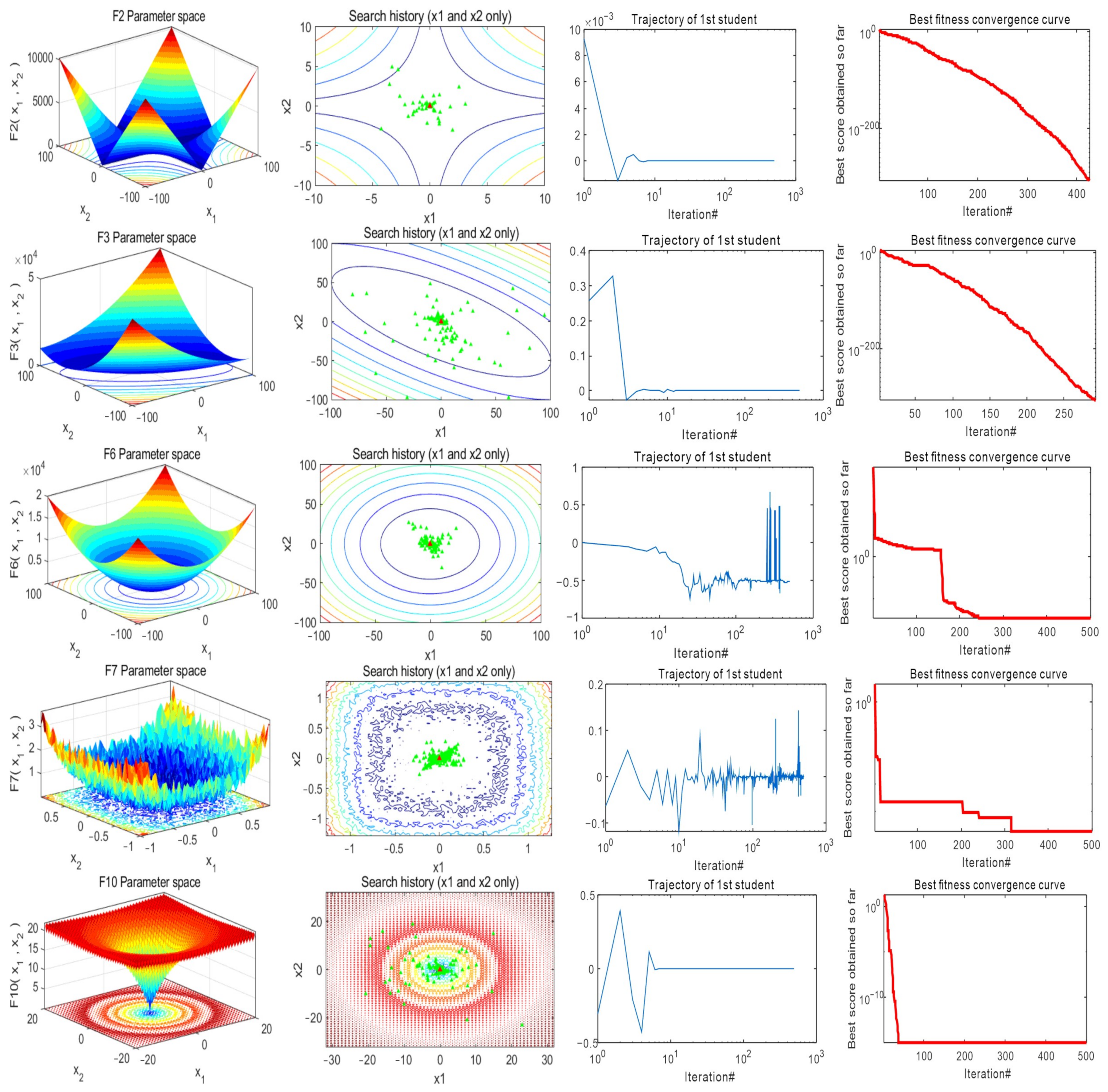
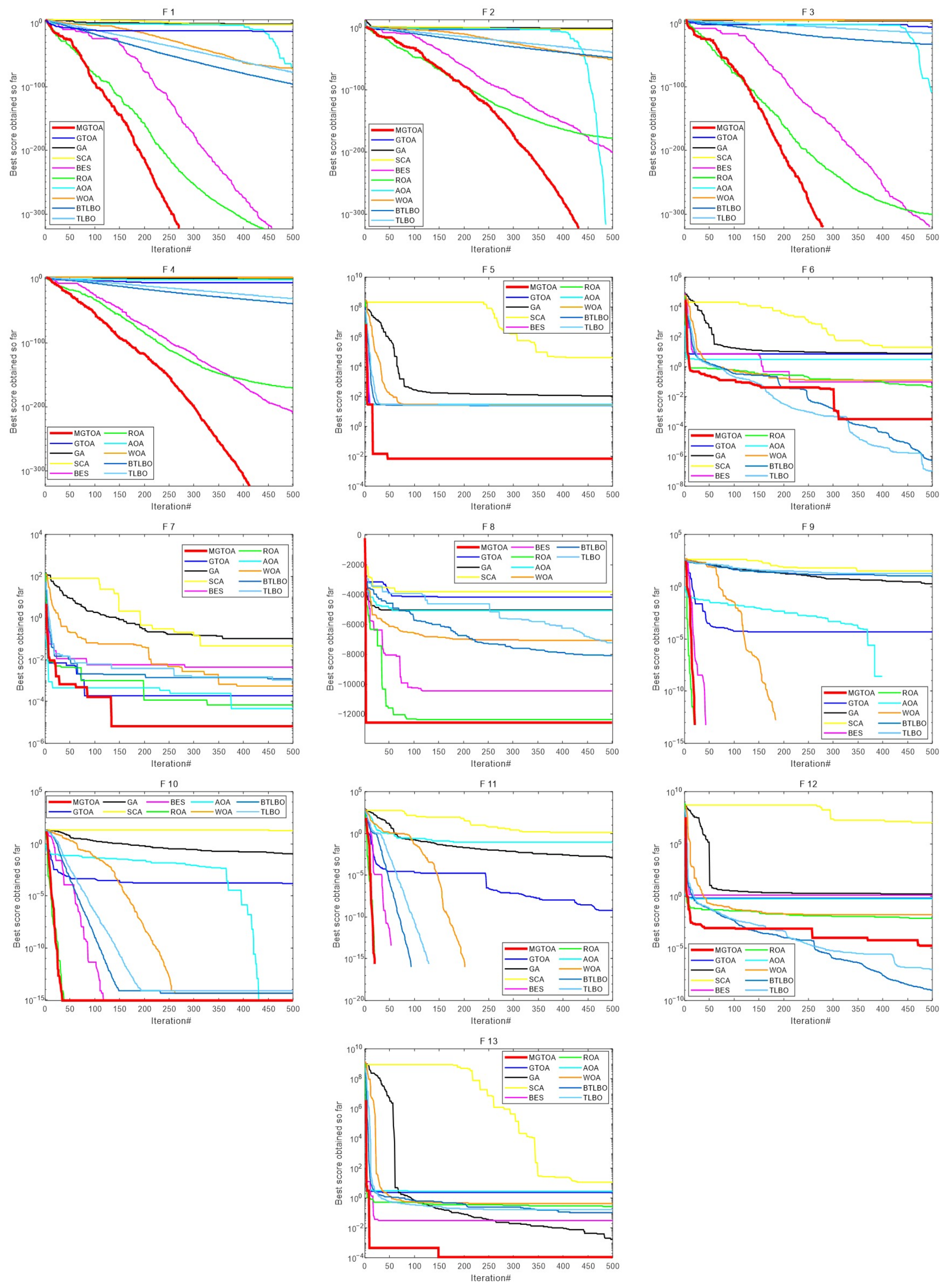
The optimization of MGTOA in different dimensions (dim = 30/500) among 23 standard benchmark functions is evaluated, and the distribution of MGTOA in some benchmark functions is shown.
Test the optimization performance of MGTOA in CEC2014.
MGTOA is compared with seven different optimization algorithms.
Six process problems verify the engineering practicability of MGTOA.

The organizational structure of this paper is as follows: Section 2 gives a brief description of GTOA, while Section 3 describes the use of operators: learning motivation (LM), random opposition-based learning (ROBL), restart strategy (RS), and gives the framework of the proposed algorithm. Section 4 and Section 5 show the algorithm’s experimental results in solving benchmark and constraint engineering problems, while Section 6 summarizes the paper.

2. Group Teaching Optimization Algorithm (GTOA)

The idea of GTOA is to improve the knowledge level of the whole class by simulating the group learning mechanism. Considering that every student has different knowledge, it is very complicated in practice. In order to integrate the idea of group teaching into the optimization algorithm, this paper assumes that the population, decision variables, and fitness values are similar to the students, the subjects provided to the students, and the student’s knowledge. The algorithm is divided into the following four phases.

2.1. Ability Grouping Phase

In order to better show the advantages of group teaching, all students will be divided into two groups according to their knowledge level, and the teacher will carry out different teaching for these two groups of students. In grouping, the relatively strong group is called elite students, and the other group is called ordinary students. Teachers will be more capable of making different teaching plans when teaching. After grouping, the gap between elite and ordinary students will become larger with the teachers’ teaching. For better teaching, the grouping of GTOA is a dynamic process, and grouping is performed again after one cycle of learning.

2.2. Teacher Phase

The teacher phase refers to students acquiring knowledge through their teachers. In GTOA, teachers make two different teaching plans for two groups of students.

Teacher phase Ⅰ: Elite students have a strong ability to accept knowledge, so teachers pay more attention to improving students’ overall average knowledge level. In addition, the differences in students’ acceptance of knowledge are also considered. Therefore, elite students will learn according to the teachers’ teaching and students’ overall knowledge level. This can effectively improve the overall knowledge level.

x_{t e a c h e r, i} = x_{i} + a \times (x_{T} - F \times (b \times M + c \times x_{i}))

(1)

M = \frac{1}{N} \sum_{i = 1}^{N} x_{i}

(2)

b + c = 1

(3)

where N is the number of students, and

x_{i}

is the ith student.

x_{T}

is a teacher. M is the average knowledge of students.

x_{t e a c h e r, i}

is the solution obtained through the teacher phase. a, b, and c are random numbers in [0, 1]. The value of F is a coefficient of 1 or 2, as done in Rao et al. [25].

Teacher phase Ⅱ: Considering that ordinary students have a general ability to accept knowledge. Teachers will pay more attention to ordinary students and tend to improve students’ knowledge levels from an individual perspective. Therefore, ordinary students will be more inclined to obtain teachers’ knowledge.

x_{t e a c h e r, i} = x_{i} + 2 \times d \times (x_{T} - x_{i})

(4)

where d is a random number between [0, 1].

In addition, students cannot guarantee that they will acquire knowledge in the teacher phase, so the minimum value is assigned to represent the knowledge level of students after the teacher phase.

x_{t e a c h e r, i} = \{\begin{cases} x_{t e a c h e r, i}, f (x_{t e a c h e r, i}) < f (x_{i}) \\ x_{i}, f (x_{t e a c h e r, i}) \geq f (x_{i}) \end{cases}

(5)

2.3. Student Phase

Students can acquire knowledge through self-study or interaction with other students in their spare time. In order to improve their knowledge level. In the spare time, students will summarize the knowledge they have learned in the teacher phase for self-study.

x_{s t u d e n t, i} = \{\begin{cases} x_{t e a c h e r, i} + e \times (x_{t e a c h e r, i} - x_{t e a c h e r, j}) + \\ g \times (x_{t e a c h e r, i} - x_{i}), f (x_{t e a c h e r, i}) < f (x_{t e a c h e r, j}) \\ x_{t e a c h e r, i} - e \times (x_{t e a c h e r, i} - x_{t e a c h e r, j}) + \\ g \times (x_{t e a c h e r, i} - x_{i}), f (x_{t e a c h e r, i}) \geq f (x_{t e a c h e r, j}) \end{cases}

(6)

where e and g are two random numbers in the range [0, 1],

x_{s t u d e n t, i}

is the knowledge of student i by learning from the student phase and

x_{t e a c h e r, j}

is the knowledge of student j by learning from the teacher phase. The random number of students j ∈ {1, 2, …, i − 1, i, …, N}. In Equation (6), the second and third items on the right mean learning from the other student and self-learning, respectively.

In addition, students cannot acquire knowledge through the student phase, so the minimum value is assigned to represent the knowledge level of students after the teacher phase.

x_{i} = \{\begin{cases} x_{t e a c h e r, i}, f (x_{t e a c h e r, i}) < f (x_{s t u d e n t, i}) \\ x_{s t u d e n t, i}, f (x_{t e a c h e r, i}) \geq f (x_{s t u d e n t, i}) \end{cases}

(7)

2.4. Teacher Allocation Phase

Selecting excellent teachers can improve students’ learning ability. Establishing a good teacher matching mechanism is important to improve students’ knowledge level. In the GWO algorithm, the average value is obtained by selecting the best three wolves and using them to guide all wolves to prey. Inspired by the hunting behavior of the GWO algorithm, the allocation of teachers is expressed by the following formula:

x_{T} = \{\begin{cases} x_{first}, f (x_{first}) \leq f (\frac{x_{first} + x_{second} + x_{third}}{3}) \\ \frac{x_{first} + x_{second} + x_{third}}{3}, f (x_{first}) > f (\frac{x_{first} + x_{second} + x_{third}}{3}) \end{cases}

(8)

where,

x_{first}

,

x_{second}

, and

x_{third}

are the students with the first, second, and third fitness values, respectively. In order to accelerate the convergence of the algorithm, elite students and ordinary students generally use the same teacher.

2.5. The Proposed Approach

Step 1: Initialization.

(1.1) Initialization parameters.

These parameters include maximum evaluation times T_max, current evaluation times t (t = 0), population size N, upper and lower bounds ub and lb of decision variables, dimension dim, and fitness function f(·).

(1.2) Initialize population.

Initialize solution x according to the test function. Each group of variables represents one student. It can be described as:

x^{} = {[x_{1}^{}, x_{2}^{}, \dots, x_{N}^{}]}^{T_{m a x}} = [\begin{matrix} x_{1, 1} & x_{1, 2} & \dots & x_{1, \dim} \\ x_{2, 1} & x_{2, 2} & \dots & x_{2, \dim} \\ ⋮ & ⋮ & ⋮ \\ x_{N, 1} & x_{N, 2} & \dots & x_{N, \dim} \end{matrix}]

(9)

x_{i}^{} = l b + (u b - l b) \times k

(10)

where k is a random number in the range [0, 1].

Step 2: Calculate fitness value.

The fitness value of the individual is calculated, and the optimal solution G is selected.

Step 3: Termination conditions

If the current iteration number t is greater than the maximum iteration number T_max, the algorithm is terminated, and the optimal solution G is output.

Step 4: Teacher allocation phase

The first three best individuals are selected. Then, the teacher

x_{T}

can be calculated by Equation (8).

Step 5: Ability grouping phase.

The students are divided into two groups based on the fitness value of the current students. The best half of the students are divided into elite group

x_{g o o d}^{}

and the remaining half into the ordinary group

x_{b a d}^{}

. The two groups share a teacher.

Step 6: Teacher phase and student phase

(6.1). For the group

x_{g o o d}^{}

, the teacher phase is implemented based on Equations (1)–(3) and (5). Then, the student phase is conducted according to Equations (6) and (7). Finally, the new students

x_{g o o d}^{}

is obtained.

(6.2) For the group

x_{b a d}^{}

, the teacher phase is implemented based on Equations (4) and (5). Then, the student phase is conducted according to Equations (6) and (7). Finally, the new students

x_{b a d}^{}

is obtained.

Step 7: Population evaluation.

Calculate the fitness value of students, select the optimal solution G, and update the current iteration number t.

t = t + 1

(11)

Then, Step 3 is executed.

3. Proposed Algorithm

3.1. Learning Motivation

Each student can acquire knowledge through self-study or communication with classmates in the student phase of the original algorithm. However, it does not fit elite students and ordinary students. Elite students have stronger learning abilities and motivation than ordinary students and are more inclined to self-study. However, ordinary students are weak in learning ability and tend to study among their classmates.

Therefore, elite students obtain learning motivation D according to Equation (12) and find a new solution through Equation (13). Ordinary students can find a new solution according to Equation (14).

D = (1 - i) / N \times \sin (2 \times π \times r)

(12)

x_{s t u d e n t, i}^{} = x_{t e a c h e r, i}^{} + D \times x_{t e a c h e r, i}^{}

(13)

where r is a random number of [0, 1].

x_{s t u d e n t, i} = \{\begin{cases} x_{t e a c h e r, i} + e \times (x_{t e a c h e r, i} - x_{t e a c h e r, j}) + g \times (x_{t e a c h e r, i} - M), f (x_{t e a c h e r, i}) < f (x_{t e a c h e r, j}) \\ x_{t e a c h e r, i} - e \times (x_{t e a c h e r, i} - x_{t e a c h e r, j}) + g \times (x_{t e a c h e r, i} - M), f (x_{t e a c h e r, i}) \geq f (x_{t e a c h e r, j}) \end{cases}

(14)

3.2. Random Opposition-Based Learning

Opposition-based learning (OBL) is a new computational intelligence scheme [30]. In the past few years, OBL has been successfully applied to various population-based evolutionary algorithms [31,32,33,34,35]. Random opposition-based learning increases the random value of [0, 1] on the basis of opposition-based learning, so as to obtain the random solution within the range of inverse solution. It not only expands the search range but also strengthens the diversity of the population so that the algorithm has a stronger exploration ability and convergence ability. The specific formula is as follows:

x n e w_{i} = (u b + l b) - (x_{T} - t) / T_{\max} \times r a n d \times x_{i}

(15)

where

x n e w_{i}^{}

represents the solution obtained after random opposition-based learning.

It is determined whether the solution obtained by the random opposition-based learning is better than the original solution:

x_{i}^{} = \{\begin{cases} x_{i}^{}, f (x_{i}^{}) \leq f (x n e w_{i}^{}) \\ x n e w_{i}^{}, f (x_{i}^{}) > f (x n e w_{i}^{}) \end{cases}

(16)

3.3. Restart Strategy (RS)

Restart strategy [36] can reassign the value of the solution which has been trapped in the local optimal state for a long time and make the poor solution jump out of the local optimal state. Adding the restart strategy can strengthen the exploration ability of the algorithm and make the algorithm converge better.

First, set the restart threshold Limit according to Equation (17). Then, set the vector trial for each solution, and record whether a better solution is obtained after each iteration. The initial value is 0. If a better solution is obtained, the corresponding trial is 0. Otherwise, the corresponding trial is increased by 1. If the vector trial is greater than the Limit, the restart strategy is executed. The Limit’s function image is shown in Figure 1.

L i m i t = \ln (t)

(17)

Figure 1. Limit schematic diagram.

The restart strategy generates two new solution T₁ and T₂, respectively, by Equations (18) and (19) and performs boundary processing by Equation (20), and then selects a better solution to replace the original solution. After that, the corresponding trial is reassigned to 0. The formula of the restart strategy is as follows:

T_{1} = l b + r a n d () \times (u b - l b)

(18)

T_{2} = r a n d () \times (u b + l b) - x_{i}

(19)

T_{2} = l b + r a n d () \times (u b - l b) i f T_{2} \geq u b | | T_{2} \leq l b

(20)

3.4. MGTOA Complexity Analysis

The time complexity depends on the number of students (N), the dimension of the given problem (dim), the number of iterations of the algorithm (T), and the evaluation cost (C). Therefore, the time complexity of MGTOA can be presented as:

\begin{array}{l} O (MGTOA) = O (define parameters) + O (population initialization) \\ + O (dunction evaluation cost) + O (location update) \end{array}

(21)

where the time complexities of the components of Equation (22) can be defined as follows:

Initialization of problem definition demands O(1) time.
Initialization of population creation demands O(N × dim) time.
Updating the population position includes the teacher and student phases and the required time O(2 × T × N × dim).
Time required for random opposition-based learning O(T × N × dim).
Time required for restart strategy O(2 × T × N × dim/Limit).
The cost time of the calculation function includes the calculation time cost of the algorithm itself, the calculation time cost of the random opposition-based learning strategy, and the calculation time cost of the restart strategy. The calculation time cost of the algorithm itself is O(T × N × C). The calculation time cost of the random opposition-based learning strategy is O(T × N × C). The calculation time cost of the restart strategy takes into account the change of the Limit value, so the time cost is O(T × N × C/Limit). The total time cost is O(2 × T × N × C + T × N × C/Limit).

Therefore, the time complexity of MGTOA is expressed as:

O (MGTOA) = O (1 + N \times d i m + T \times N \times C \times (2 + \frac{1}{L i m i t}) + T \times N \times d i m \times (3 + \frac{2}{L i m i t}))

(22)

Because 1 ≪ T × N × C, 1 ≪ T × N × dim, N × dim ≪ T × N × C, and N × dim ≪ T × N × dim, Equation (22) can be simplified to Equation (23).

O (MGTOA) ≅ O (T \times N \times C \times (2 + \frac{1}{L i m i t}) + T \times N \times d i m \times (3 + \frac{2}{L i m i t}))

(23)

It can be seen from the above analysis that the time complexity of MGTOA is improved compared with GTOA, but after these strategies are added, the optimization effect of MGTOA is significantly improved. The following experiments also prove the feasibility of MGTOA.

3.5. MGTOA Implementation

Combining GTOA with the three strategies mentioned above, an improved group teaching optimization algorithm (MGTOA) is presented. Through the above three improvement strategies, the exploration ability of MGTOA is strengthened, making the calculation more global. Pseudocode is shown in Algorithm 1.

Algorithm 1 Pseudo-code of MGTOA

1. Initialization parameters t, T_max, ub, lb, N, dim.

2. Initialize population x according to Equations (9) and (10).

3. The fitness values of all individuals are calculated, and the optimal solution G is selected.

4. While t < T_max

5. Define the teacher according to Equation (8).

6. Students are divided into elite students (X_good) and ordinary students (X_bad). The number of elite students is N_good.

7. for i = 1:N

8. if i < N_good

9. The teacher phase is achieved according to Equations (1)–(3), and (5).

10. else

11. The teacher phase is realized according to Equations (4) and (5).

12. end

13. Carry out boundary processing for the updated students.

14. Calculate the average knowledge level of elite students (M)

15. if i < N_good

16. for j = 1:dim

17. The elite students get the learning motivation D according to Equation (12) and carry out the student phase through Equations (13) and (7).

18. end

19. else

20. Ordinary students carry out the student phase according to Equations (14) and (7).

21. end

22. end

23. Carry out boundary processing for the updated students.

24. An inverse solution is generated using a random opposition-based learning strategy by Equation (15), and the student position is updated according to Equation (16).

25. Calculate the new fitness value of the students and judge whether it is better. If it is better, replace the fitness value and the corresponding trial = 0. Otherwise, trial will add 1

26. Define Limit according to Equation (17).

27. for i = 1:N

28. while trial(i) < Limit

29. T₁ and T₂ are generated by Equations (18) and (19), and T₂ is subjected to boundary processing using Equation (20). Assign a smaller position to x_i.

30. trial(i) = 0

31. end

32. end

33. t = t + 1

34. end

The MGTOA flow chart is shown in Figure 2.

Figure 2. Flowchart for proposed MGTOA.

4. Experimental Results and Discussion

All the experiments in this paper are completed on a computer with the 11th Gen Intel(R) Core(TM) i7-11700 processor with the primary frequency of 2.50GHz, 16GB memory, and the operating system of 64-bit windows 11 using matlab2021a.

In this section, MGTOA is brought into two different types of benchmark functions to evaluate the performance of the modified algorithm. First, the performance of MGTOA in solving simple optimization problems is evaluated by experiments on 23 standard benchmark functions. After that, it is verified by CEC 2014 test function, which contains 30 test functions. Finally, in order to verify that the proposed MGTOA has better performance, the MGTOA is compared with GTOA [28], Genetic Algorithms (GA) [11], Sine Cosine Algorithm (SCA) [37], Bald Eagle Search (BES) [38], Remora Optimization Algorithm (ROA) [10], Arithmetic Optimization Algorithm (AOA) [39], Whale Optimization Algorithm (WOA) [9], Teaching Learning-Based Optimization Algorithm (TLBO) [25], and Balanced Teaching Learning-Based Optimization Algorithm (BTLBO) [40]. The parameter settings of these algorithms are shown in Table 1.

Table 1. Parameter settings for the comparative algorithms.

4.1. Experiments on Standard Benchmark Functions

In this section, the performance of MGTOA is tested using 23 mathematical benchmark functions and compared with other nine algorithms. This benchmark contains seven unimodal, six multimodal, and ten fixed-dimension multimodal functions. As shown in Table 2, where F is the mathematical function, dim is the dimension, Range is the interval of the search space, and F_min is the optimal value the corresponding function can achieve. Among the 23 standard benchmark functions, set the population number N = 30, the maximum number of iterations T = 500, and the dimension dim = 30/500. All the algorithms run independently 30 times to obtain the optimal fitness value, the average fitness value, and the standard deviation.

Table 2. Details of 23 benchmark functions.

Figure 3 shows a partial graph of 23 benchmark functions, the historical distribution of MGTOA in the benchmark function, the historical trajectory of the first individual, and the convergence curve of MGTOA. It can be clearly seen from the figure that MGTOA obtained the results and position distribution after each optimization.

Figure 3. Results of MGTOA in 23 benchmark functions.

Table 3, Table 4 and Table 5 are the statistical charts of 23 benchmark functions of MGTOA and nine other comparison algorithms, and the best values obtained are shown in bold black. It can be seen that MGTOA has been significantly improved compared with other algorithms and has achieved good results in 23 benchmark functions. In F1–F4, the statistical value of MGTOA has been significantly improved compared with GTOA, and the fitness value has reached the theoretical optimum. BES has achieved good results in F1, and AOA has achieved good results in F2. Other comparison algorithms are insufficient in F1–F4. In 30 dimensions, MGTOA did not obtain the minimum fitness value in F6 and F12, which indicates that MGTOA is insufficient. However, in the 500 dimensions, MGTOA has achieved the minimum fitness value. This shows that the optimization performance of MGTOA is more stable and has good effects in different dimensions. TLBO and BTLBO cannot guarantee good effects in high dimensions. Among other functions, MGTOA has achieved good results. BES and ROA have achieved good results in F9–F11, but other functions are not as effective as MGTOA. In Table 5, because the function is relatively simple, many algorithms can obtain better fitness values. MGTOA obtains the best fitness value in most functions and has good stability. ROA, WOA, BTLBO, and TLBO also achieved good results. The performance of other algorithms is relatively weak, and they only have good results in some functions. The above analysis verifies that MGTOA has a good effect on 23 benchmark functions.

In order to more intuitively see the optimization ability of each algorithm, the convergence curves of each algorithm in 23 mathematical benchmark functions are shown in Figure 4, Figure 5 and Figure 6, which can more intuitively understand the convergence effect of each algorithm. From F1–F4, it can be seen that the MGTOA optimization effect is obviously superior to other algorithms. MGTOA has good convergence ability in the early stage of the algorithm and can quickly find the optimal value. In Figure 4, MGTOA is inferior to TLBO and BTLBO in F6 and F12. However, in Figure 5, the value obtained by MGTOA is significantly smaller, and other algorithms cannot converge. It shows that MGTOA has better performance when dealing with high-dimensional problems. In other functions, MGTOA can converge quickly and get a good value. It is further proved that MGTOA has better optimization ability in 23 benchmark functions.

Figure 4. Convergence curves for the optimization algorithms for standard benchmark functions (F1–F13) with dim = 30.

Figure 5. Convergence curves for the optimization algorithms for standard benchmark functions (F1–F13) with dim = 500.

Figure 6. Convergence curves for the optimization algorithms for standard benchmark functions (F14–F23).

In addition, the Wilcoxon rank sum test is a nonparametric statistical test method that can find more complex data distribution. The general data analysis is only aimed at the average value and standard deviation of the current data and is not compared with the data of multiple algorithms runs. Therefore, the Wilcoxon rank sum test is required for further verification. Table 6 shows the experimental results of MGTOA and nine other different algorithms running 30 times in 23 mathematical benchmark functions. Among them, the significance level is 5%. The value of less than 5% indicates a significant difference between the two algorithms. Otherwise, it indicates that the two algorithms are close. It can be seen from the table that the p of most functions is less than 0.05, but some functions are greater than 0.05. MGTOA has four functions p = 1 compared with BES. MGTOA has three functions p = 1 compared with ROA. Compared with AOA, MGTOA has three functions p = 1 when dim = 30. This is because both these algorithms and MGTOA can find the theoretical optimal fitness value in these functions. Compared with MGTOA, WOA, BTLBO and TLBO have many p less than 0.05 in F9–F11. It shows that the optimization effect of these algorithms in this function is similar. However, in most cases, the p obtained by MGTOA and other algorithms is less than 0.05. In general, MGTOA has achieved good results in the Wilcoxon rank sum test.

Table 3. Results of benchmark functions (F1–F13) under 30 dimensions.

F	Metric	MGTOA	GTOA [28]	GA [11]	SCA [37]	BES [38]	ROA [10]	AOA [39]	WOA [9]	BTLBO [40]	TLBO [25]
F1	min	0	1.13 × 10⁻¹⁴	9.69 × 10⁻³	8.36 × 10⁻²	0	0	3.05 × 10⁻¹⁹³	6.03 × 10⁻⁸⁶	1.47 × 10⁻⁹⁷	5.3 × 10⁻⁸¹
	mean	0	5.92 × 10⁻⁶	2.37 × 10⁻²	16.5	0	2.99 × 10⁻³¹⁹	2.56 × 10⁻³⁰	2.21 × 10⁻⁶⁸	9.71 × 10⁻⁹⁶	6.99 × 10⁻⁷⁹
	std	0	2.42 × 10⁻⁵	6.57 × 10⁻³	36.5	0	0	1.40 × 10⁻²⁹	1.21 × 10⁻⁶⁷	2.03 × 10⁻⁹⁵	1.76 × 10⁻⁷⁸
F2	min	0	3.43 × 10⁻⁷	3.64 × 10⁻¹	1.47 × 10⁻⁶	2.38 × 10⁻²²⁹	1.70 × 10⁻¹⁸²	0	1.7 × 10⁻⁵⁹	3.54 × 10⁻⁴⁹	1.24 × 10⁻⁴⁰
	mean	0	5.83 × 10⁻⁴	4.91 × 10⁻¹	1.43 × 10⁻²	2.43 × 10⁻¹⁶¹	2.91 × 10⁻¹⁶²	0	1.92 × 10⁻⁴⁹	2.63 × 10⁻⁴⁸	5.07 × 10⁻⁴⁰
	std	0	1.67 × 10⁻³	7.28 × 10⁻²	2.31 × 10⁻²	1.33 × 10⁻¹⁶⁰	1.56 × 10⁻¹⁶¹	0	8.92 × 10⁻⁴⁹	2.63 × 10⁻⁴⁸	5.35 × 10⁻⁴⁰
F3	min	0	3.58 × 10⁻¹¹	9.24 × 10³	1.82 × 10³	0	1.59 × 10⁻³²¹	1.96 × 10⁻¹³²	2.11 × 10⁴	2.29 × 10⁻³⁷	1.15 × 10⁻¹⁹
	mean	0	5.10 × 10⁻⁴	2.16 × 10⁴	8.87 × 10³	1.76 × 10⁻²⁷	1.02 × 10⁻²⁸⁴	2.9 × 10⁻³	4.08 × 10⁴	5.54 × 10⁻³³	1.3 × 10⁻¹⁶
	std	0	2.63 × 10⁻³	8.05 × 10³	5.64 × 10³	9.64 × 10⁻²⁷	0	5.97 × 10⁻³	1.37 × 10⁴	1.51 × 10⁻³²	5.06 × 10⁻¹⁶
F4	min	0	3.04 × 10⁻⁷	2.15 × 10⁻¹	9.56	9.19 × 10⁻²³⁷	7.35 × 10⁻¹⁸⁰	7.99 × 10⁻⁵¹	8.24	3.52 × 10⁻⁴⁰	2.09 × 10⁻³³
	mean	0	4.8 × 10⁻⁴	2.82 × 10⁻¹	36.4	9.34 × 10⁻¹⁷¹	4.87 × 10⁻¹⁵²	2.25 × 10⁻²	54.0	2.27 × 10⁻³⁹	1.43 × 10⁻³²
	std	0	8.52 × 10⁻⁴	3.86 × 10⁻²	13.1	0	2.63 × 10⁻¹⁵¹	2.12 × 10⁻²	24.3	3 × 10⁻³⁹	1.30 × 10⁻³²
F5	min	5.39 × 10⁻⁶	28.9	25.5	44.6	9.27 × 10⁻⁴	26.6	27.8	2.73 × 10⁻¹	2.29 × 10⁻¹	23.4
	mean	8.90 × 10⁻¹	28.9	70.7	8.17 × 10⁴	21.8	27.1	28.5	28.0	23.9	24.7
	std	4.7	2.79 × 10⁻²	30.7	1.83 × 10⁵	12	3.63 × 10⁻¹	3.08 × 10⁻¹	4.64 × 10⁻¹	6.67 × 10⁻¹	6.32 × 10⁻¹
F6	min	1.4 × 10⁻⁵	4.42	7.83	5.52	3.21 × 10⁻⁴	1.69 × 10⁻²	2.69	1.14 × 10⁻¹	4.84 × 10⁻⁹	2.66 × 10⁻⁸
	mean	1.11 × 10⁻³	5.67	8.07	25.8	1.35	1.04 × 10⁻¹	3.24	4.47 × 10⁻¹	1.06 × 10⁻⁶	1.17 × 10⁻⁶
	std	1.18 × 10⁻³	7.71 × 10⁻¹	1.38 × 10⁻¹	49	2.8	1.21 × 10⁻¹	2.74 × 10⁻¹	3.27 × 10⁻¹	2.64 × 10⁻⁶	3.77 × 10⁻⁶
F7	min	4.97 × 10⁻⁸	1.06 × 10⁻⁴	8.88 × 10⁻²	1.7 × 10⁻²	2.03 × 10⁻³	4.43 × 10⁻⁶	2.47 × 10⁻⁷	9.51 × 10⁻⁵	3.60 × 10⁻⁴	5.57 × 10⁻⁴
	mean	3.79 × 10⁻⁵	4.49 × 10⁻⁴	1.98 × 10⁻¹	1.1 × 10⁻¹	6.19 × 10⁻³	1.85 × 10⁻⁴	8 × 10⁻⁵	3.32 × 10⁻³	8.10 × 10⁻⁴	1.13 × 10⁻³
	std	3.29 × 10⁻⁵	2.6 × 10⁻⁴	7.02 × 10⁻²	1.08 × 10⁻¹	3.54 × 10⁻³	1.71 × 10⁻⁴	8.71 × 10⁻⁵	3.65 × 10⁻³	4.16 × 10⁻⁴	5.20 × 10⁻⁴
F8	min	−1.26 × 10⁴	−6.16 × 10³	−5.94 × 10³	−4.73 × 10³	−9.97 × 10³	−1.26 × 10⁴	−6.19 × 10³	−1.26 × 10⁴	−9.87 × 10³	−9.45 × 10³
	mean	−1.26 × 10⁴	−5.09 × 10³	−4.73 × 10³	−3.78 × 10³	−5.80 × 10³	−1.24 × 10⁴	−5.41 × 10³	−1.03 × 10⁴	−7.60 × 10³	−7.67 × 10³
	std	6.00 × 10⁻²	6.87 × 10²	6.85 × 10²	3.61 × 10²	3.23 × 10³	3.26 × 10²	4.37 × 10²	1.68 × 10³	1.01 × 10³	1.21 × 10³
F9	min	0	5.7 × 10⁻¹¹	1.37	1.25 × 10⁻¹	0	0	0	0	8.04	9.95
	mean	0	2.44 × 10⁻⁵	2.74	34.7	0	0	0	7.58 × 10⁻¹⁵	19.0	14.4
	std	0	8.93 × 10⁻⁵	8.29 × 10⁻¹	30.5	0	0	0	2.47 × 10⁻¹⁴	8.82	6.97
F10	min	8.88 × 10⁻¹⁶	2.55 × 10⁻⁸	9.25 × 10⁻²	4.78 × 10⁻²	8.88 × 10⁻¹⁶	8.88 × 10⁻¹⁶	8.88 × 10⁻¹⁶	8.88 × 10⁻¹⁶	4.44 × 10⁻¹⁵	4.44 × 10⁻¹⁵
	mean	8.88 × 10⁻¹⁶	3.36 × 10⁻⁴	1.33 × 10⁻¹	15.4	1.13 × 10⁻¹⁵	8.88 × 10⁻¹⁶	8.88 × 10⁻¹⁶	4.8 × 10⁻¹⁵	5.03 × 10⁻¹⁵	6.34 × 10⁻¹⁵
	std	0	7.52 × 10⁻⁴	3.09 × 10⁻²	7.96	9.01 × 10⁻¹⁶	0	0	2.35 × 10⁻¹⁵	1.35 × 10⁻¹⁵	1.8 × 10⁻¹⁵
F11	min	0	1.06 × 10⁻¹²	6.76 × 10⁻⁴	1.83 × 10⁻²	0	0	2.66 × 10⁻²	0	0	0
	mean	0	1.11 × 10⁻⁵	8.6 × 10⁻²	9.91 × 10⁻¹	0	0	1.88 × 10⁻¹	1.18 × 10⁻²	0	2.76 × 10⁻⁶
	std	0	4.1 × 10⁻⁵	2.7 × 10⁻¹	3.07 × 10⁻¹	0	0	1.59 × 10⁻¹	6.45 × 10⁻²	0	1.51 × 10⁻⁵
F12	min	3.52 × 10⁻⁷	3.44 × 10⁻¹	1.55	8.5 × 10⁻¹	1.48 × 10⁻⁶	2.78 × 10⁻³	3.98 × 10⁻¹	7.12 × 10⁻³	2.49 × 10⁻¹⁰	5.78 × 10⁻¹¹
	mean	2.15 × 10⁻⁵	6.21 × 10⁻¹	1.72	5.51 × 10⁴	1.33 × 10⁻¹	1.07 × 10⁻²	5.24 × 10⁻¹	4.39 × 10⁻²	1.02 × 10⁻⁸	1.26 × 10⁻⁸
	std	2.01 × 10⁻⁵	1.88 × 10⁻¹	5.17 × 10⁻²	1.74 × 10⁵	3.28 × 10⁻¹	6.41 × 10⁻³	4.53 × 10⁻²	1 × 10⁻¹	2.68 × 10⁻⁸	3.63 × 10⁻⁸
F13	min	1.17 × 10⁻⁶	2.45	1.37 × 10⁻³	4.82	4.66 × 10⁻⁵	7.92 × 10⁻²	2.65	1.72 × 10⁻¹	2.13 × 10⁻⁷	1.59 × 10⁻⁷
	mean	2.65 × 10⁻⁴	2.87	4.46 × 10⁻³	1.89 × 10⁵	1.22	2.4 × 10⁻¹	2.82	5.69 × 10⁻¹	9.96 × 10⁻²	8.4 × 10⁻²
	std	3.56 × 10⁻⁴	2.26 × 10⁻¹	3.29 × 10⁻³	5.58 × 10⁵	1.47	1.38 × 10⁻¹	9.65 × 10²	2.44 × 10⁻¹	8.27 × 10⁻²	1.23 × 10⁻¹

Table 4. Results of benchmark functions (F1–F13) under 500 dimensions.

F	Metric	MGTOA	GTOA [28]	GA [11]	SCA [37]	BES [38]	ROA [10]	AOA [39]	WOA [9]	BTLBO [40]	TLBO [25]
F1	min	0	3.10 × 10⁻¹³	67.2	9.04 × 10⁴	0	0	5.60 × 10⁻¹	2.86 × 10⁻⁸¹	3.95 × 10⁻⁸⁵	1.12 × 10⁻⁶⁸
	mean	0	1.37 × 10⁻⁴	70.6	2.03 × 10⁵	0	2.17 × 10⁻³¹⁸	6.43 × 10⁻¹	1.49 × 10⁻⁶⁷	9.97 × 10⁻⁸⁴	1.34 × 10⁻⁶⁷
	std	0	6.23 × 10⁻⁴	2.63	8.08 × 10⁴	0	0	4.45 × 10⁻²	8.06 × 10⁻⁶⁷	1.03 × 10⁻⁸³	1.78 × 10⁻⁶⁷
F2	min	0	2.76 × 10⁻⁷	1.35 × 10²	31.8	6.28 × 10⁻²²⁵	9.78 × 10⁻¹⁷⁷	3.81 × 10⁻¹²	9.26 × 10⁻⁵⁵	4.58 × 10⁻⁴³	7.22 × 10⁻³⁵
	mean	0	5.98 × 10⁻³	1.40 × 10²	1.07 × 10²	2.93 × 10⁻¹⁵³	3.10 × 10⁻¹⁵¹	1.82 × 10⁻³	1.3 × 10⁻⁴⁷	2.06 × 10⁻⁴²	2.16 × 10⁻³⁴
	std	0	1.28 × 10⁻²	3.03	57.5	1.6 × 10⁻¹⁵²	1.70 × 10⁻¹⁵⁰	1.7 × 10⁻³	6.57 × 10⁻⁴⁷	1.53 × 10⁻⁴²	1.35 × 10⁻³⁴
F3	min	0	9.38 × 10⁻⁹	4.86 × 10⁵	5.09 × 10⁶	0	7.16 × 10⁻²⁹⁹	13.7	1.88 × 10⁷	2.77 × 10⁻¹³	4.58 × 10⁻³
	mean	0	1.23 × 10⁻¹	7.17 × 10⁵	6.75 × 10⁶	8.68 × 10⁵	5.08 × 10⁻²⁶¹	3.42 × 10³	3.32 × 10⁷	5.59 × 10⁻⁶	3.8 × 10⁻¹
	std	0	5.99 × 10⁻¹	1.39 × 10⁵	1.42 × 10⁶	4.43 × 10⁶	0	1.85 × 10⁴	1.23 × 10⁷	2.41 × 10⁻⁵	1.27
F4	min	0	5.2 × 10⁻⁸	9.52 × 10⁻¹	98.6	8.66 × 10⁻²¹⁷	2.23 × 10⁻¹⁷³	1.63 × 10⁻¹	55.1	2.13 × 10⁻³⁵	5.69 × 10⁻²⁸
	mean	0	2.8 × 10⁻⁴	9.71 × 10⁻¹	99.0	1.3 × 10⁻¹²⁸	7.74 × 10⁻¹⁵²	1.81 × 10⁻¹	81.3	1.22 × 10⁻³⁴	1.42 × 10⁻²⁷
	std	0	4.51 × 10⁻⁴	1.04 × 10⁻²	3.42 × 10⁻¹	7.13 × 10⁻¹²⁸	4.13 × 10⁻¹⁵¹	1.65 × 10⁻²	22.1	8.42 × 10⁻³⁵	9.58 × 10⁻²⁸
F5	min	4.12 × 10⁻⁸	4.99 × 10²	4.90 × 10³	1.12 × 10⁹	1.13 × 10²	4.94 × 10²	4.99 × 10²	4.96 × 10²	4.96 × 10²	4.96 × 10²
	mean	1.16 × 10²	4.99 × 10²	5.14 × 10³	1.95 × 10⁹	4.32 × 10²	4.95 × 10²	4.99 × 10²	4.96 × 10²	4.97 × 10²	4.97 × 10²
	std	2.14 × 10²	3.20 × 10⁻²	1.76 × 10²	5.05 × 10⁸	1.67 × 10²	2.94 × 10⁻¹	1.03 × 10⁻¹	4.20 × 10⁻¹	6.30 × 10⁻¹	4 × 10⁻¹
F6	min	9.08 × 10⁻⁵	1.22 × 10²	3.35 × 10²	7.45 × 10⁴	1.14 × 10⁻²	7.29	1.14 × 10²	20.3	70	71.6
	mean	16.8	1.23 × 10²	3.45 × 10²	2.42 × 10⁵	30.6	15.3	1.16 × 10²	32.6	75.4	75.5
	std	35.3	7.36 × 10⁻¹	5.84	9.01 × 10⁴	53	6.51	1.38	9.53	2.39	2.11
F7	min	2.6 × 10⁻⁸	7.82 × 10⁻⁵	4.30 × 10³	9.38 × 10³	8.2 × 10⁻⁴	5.87 × 10⁻⁶	1.21 × 10⁻⁵	8.52 × 10⁻⁵	7.16 × 10⁻⁴	8.04 × 10⁻⁴
	mean	3.43 × 10⁻⁵	6.1 × 10⁻⁴	4.56 × 10³	1.44 × 10⁴	5.75 × 10⁻³	2.08 × 10⁻⁴	1.06 × 10⁻⁴	4.37 × 10⁻³	1.3 × 10⁻³	1.66 × 10⁻³
	std	3.22 × 10⁻⁵	6.31 × 10⁻⁴	2.74 × 10²	3.4 × 10³	4.01 × 10⁻³	1.66 × 10⁻⁴	9.94 × 10⁻⁵	5.6 × 10⁻³	4.27 × 10⁻⁴	5.37 × 10⁻⁴
F8	min	−2.09 × 10⁵	−2.85 × 10⁴	−3.63 × 10⁴	−1.73 × 10⁴	−2.08 × 10⁵	−2.09 × 10⁵	−2.58 × 10⁴	−2.09 × 10⁵	−7.28 × 10⁴	−6.17 × 10⁴
	mean	−2.09 × 10⁵	−2.15 × 10⁴	−3.29 × 10⁴	−1.53 × 10⁴	−1.61 × 10⁵	−2.05 × 10⁵	−2.3 × 10⁴	−1.7 × 10⁵	−3.39 × 10⁴	−4.39 × 10⁴
	std	1.18	3.12 × 10³	1.91 × 10³	1.23 × 10³	2.49 × 10⁴	1.02 × 10⁴	1.58 × 10³	3.1 × 10⁴	1.10 × 10⁴	1.21 × 10⁴
F9	min	0	0	2.26 × 10³	4.19 × 10²	0	0	0	0	0	0
	mean	0	9.27 × 10⁻⁵	2.41 × 10³	1.14 × 10³	0	0	8.08 × 10⁻⁶	9.09 × 10⁻¹⁴	0	0
	std	0	3.52 × 10⁻⁴	72.5	5.78 × 10²	0	0	7.61 × 10⁻⁶	3.66 × 10⁻¹³	0	0
F10	min	8.88 × 10⁻¹⁶	2.26 × 10⁻⁸	2.85	10.7	8.88 × 10⁻¹⁶	8.88 × 10⁻¹⁶	7.09 × 10⁻³	8.88 × 10⁻¹⁶	7.99 × 10⁻¹⁵	7.99 × 10⁻¹⁵
	mean	8.88 × 10⁻¹⁶	2.84 × 10⁻⁴	2.91	18.4	8.88 × 10⁻¹⁶	8.88 × 10⁻¹⁶	8.02 × 10⁻³	4.91 × 10⁻¹⁵	7.99 × 10⁻¹⁵	2.22
	std	0	5.35 × 10⁻⁴	2.92 × 10⁻²	4.11	0	0	4.3 × 10⁻⁴	2.23 × 10⁻¹⁵	0	4.17
F11	min	0	2.10 × 10⁻¹²	2.28 × 10⁻¹	1.13 × 10³	0	0	6.52 × 10³	0	0	0
	mean	0	4.72 × 10⁻⁵	3.05 × 10⁻¹	2.08 × 10³	0	0	9.99 × 10³	3.7 × 10⁻¹⁸	0	3.7 × 10⁻¹⁸
	std	0	2.56 × 10⁻⁴	2.66 × 10⁻¹	7.11 × 10²	0	0	3.09 × 10³	2.03 × 10⁻¹⁷	0	2.03 × 10⁻¹⁷
F12	min	1.69 × 10⁻⁸	1.09	2.73	4.03 × 10⁹	1.24 × 10⁻⁵	9.45 × 10⁻³	1.07	3.97 × 10⁻²	3.84 × 10⁻¹	3.67 × 10⁻¹
	mean	1.08 × 10⁻⁵	1.14	2.80	6.28 × 10⁹	2.42 × 10⁻¹	4.54 × 10⁻²	1.08	1.01 × 10⁻¹	4.3 × 10⁻¹	4.27 × 10⁻¹
	std	2.10 × 10⁻⁵	3.37 × 10⁻²	4.75 × 10⁻²	1.36 × 10⁹	4.89 × 10⁻¹	2.79 × 10⁻²	1.2 × 10⁻²	5.11 × 10⁻²	2.75 × 10⁻²	2.96 × 10⁻²
F13	min	5.42 × 10⁻¹¹	50	10.2	6.62 × 10⁹	3.46 × 10⁻³	3.08	50.1	10.7	49.8	49.8
	mean	1.87 × 10⁻³	50	10.8	1.06 × 10¹⁰	12.2	8.69	50.2	19.3	49.8	49.8
	std	5.68 × 10⁻³	4.52 × 10⁻³	4.73 × 10⁻¹	2.11 × 10⁹	21.1	3.88	4.54 × 10⁻²	6.02	1.01 × 10⁻²	8.82 × 10⁻³

Table 5. Results of benchmark functions (F14–F23).

F	Metric	MGTOA	GTOA [28]	GA [11]	SCA [37]	BES [38]	ROA [10]	AOA [39]	WOA [9]	BTLBO [40]	TLBO [25]
F14	min	9.98 × 10⁻¹	9.98 × 10⁻¹	2.98	9.98 × 10⁻¹	9.98 × 10⁻¹	9.98 × 10⁻¹	9.98 × 10⁻¹	9.98 × 10⁻¹	9.98 × 10⁻¹	9.98 × 10⁻¹
	mean	9.98 × 10⁻¹	1.16	9.43	1.83	3.06	5.75	10.2	3.68	9.98 × 10⁻¹	9.98 × 10⁻¹
	std	3.38 × 10⁻¹¹	5.27 × 10⁻¹	3.58	1.89	1.39	5.05	4.05	3.47	0	0
F15	min	3.07 × 10⁻⁴	3.07 × 10⁻⁴	4.35 × 10⁻⁴	3.94 × 10⁻⁴	3.14 × 10⁻⁴	3.08 × 10⁻⁴	3.54 × 10⁻⁴	3.19 × 10⁻⁴	3.07 × 10⁻⁴	3.07 × 10⁻⁴
	mean	3.08 × 10⁻⁴	1.89 × 10⁻³	1.29 × 10⁻²	9.83 × 10⁻⁴	7.02 × 10⁻³	4.32 × 10⁻⁴	1.22 × 10⁻²	7.49 × 10⁻⁴	3.25 × 10⁻⁴	3.50 × 10⁻⁴
	std	2.54 × 10⁻⁷	5.34 × 10⁻³	2.75 × 10⁻²	3.98 × 10⁻⁴	8.72 × 10⁻³	2.27 × 10⁻⁴	2.66 × 10⁻²	5.11 × 10⁻⁴	7.35 × 10⁻⁵	1.19 × 10⁻⁴
F16	min	−1.03	−1.03	−1.03	−1.03	−1.03	−1.03	−1.03	−1.03	−1.03	−1.03
	mean	−1.03	−1.03	−1.00	−1.03	−9.54 × 10⁻¹	−1.03	−1.03	−1.03	−1.03	−1.03
	std	5.25 × 10⁻¹⁶	6 × 10⁻¹⁶	2.07 × 10⁻²	8.02 × 10⁻⁵	2.25 × 10⁻¹	1.25 × 10⁻⁷	1.21 × 10⁻⁷	2.04 × 10⁻⁹	6.78 × 10⁻¹⁶	6.65 × 10⁻¹⁶
F17	min	3.98 × 10⁻¹	3.98 × 10⁻¹	4.50 × 10⁻¹	3.98 × 10⁻¹	3.98 × 10⁻¹	3.98 × 10⁻¹	3.98 × 10⁻¹	3.98 × 10⁻¹	3.98 × 10⁻¹	3.98 × 10⁻¹
	mean	3.98 × 10⁻¹	3.98 × 10⁻¹	1.50	3.99 × 10⁻¹	5.81 × 10⁻¹	3.98 × 10⁻¹	3.98 × 10⁻¹	3.98 × 10⁻¹	3.98 × 10⁻¹	3.98 × 10⁻¹
	std	6.21 × 10⁻⁷	0	1.48	1.6 × 10⁻³	6.48 × 10⁻¹	6.34 × 10⁻⁶	7.93 × 10⁻⁸	1.48 × 10⁻⁵	0	0
F18	min	3	3	3.2	3	3	3	3	3	3	3
	mean	3	3	29.5	3	4.39	3	9.3	3	3	3
	std	2.06 × 10⁻⁵	8.4 × 10⁻¹⁵	22.2	1.33 × 10⁻⁴	1.51	1.61 × 10⁻⁴	11.6	1.71 × 10⁻⁴	1.31 × 10⁻¹⁵	9.79 × 10⁻¹⁶
F19	min	−3.86	−3.86	−3.86	−3.86	−3.85	−3.86	−3.86	−3.86	−3.86	−3.86
	mean	−3.86	−3.86	−3.71	−3.85	−3.65	−3.86	−3.85	−3.86	−3.86	−3.86
	std	9.49 × 10⁻⁶	2.63 × 10⁻¹⁵	5.48 × 10⁻¹	1.09 × 10⁻²	1.89 × 10⁻¹	2.8 × 10⁻³	5.9 × 10⁻³	7.31 × 10⁻³	2.71 × 10⁻¹⁵	2.71 × 10⁻¹⁵
F20	min	−3.32	−3.32	−3.32	−3.11	−3.19	−3.32	−3.17	−3.32	−3.32	−3.32
	mean	−3.29	−3.26	−3.28	−2.70	−2.91	−3.22	−3.04	−3.22	−3.3	−3.31
	std	5.27 × 10⁻²	7.66 × 10⁻²	5.55 × 10⁻²	5.27 × 10⁻¹	2.4 × 10⁻¹	1.24 × 10⁻¹	8.89 × 10⁻²	1.71 × 10⁻¹	3.67 × 10⁻²	3.71 × 10⁻²
F21	min	−10.2	−10.2	−5.05	−7.36	−10.2	−10.2	−6.85	−10.2	−10.2	−10.2
	mean	−10.2	−8	−1.47	−2.27	−6.55	−10.1	−3.93	−7.94	−10.1	−9.56
	std	2.90 × 10⁻⁴	2.75	1.49	2.06	2.76	1.6 × 10⁻²	1.72	2.79	7.74 × 10⁻²	1.81
F22	min	−10.4	−10.4	−5.07	−5.62	−10.4	−10.4	−6.05	−10.4	−10.4	−10.4
	mean	−10.4	−8.04	−1.67	−3.29	−5.43	−10.4	−3.38	−7.76	−10.4	−10
	std	1.29 × 10⁻⁴	2.97	1.25	1.85	2.61	2.41 × 10⁻²	1.49	2.91	7.38 × 10⁻¹⁶	1.35
F23	min	−10.5	−10.5	−5.13	−5.93	−10.5	−10.5	−6.69	−10.5	−10.5	−10.5
	mean	−10.5	−7.98	−1.76	−3.73	−5.55	−10.5	−3.52	−6.27	−10.3	−10.1
	std	1.28 × 10⁻⁴	3.24	1.40	1.54	2.73	2.1 × 10⁻²	1.26	3.26	1.21	1.74

Table 6. Experimental results of Wilcoxon rank sum test on 23 standard benchmark functions.

F	dim	MGTOA vs. GTOA [28]	MGTOA vs. GA [11]	MGTOA vs. SCA [37]	MGTOA vs. BES [38]	MGTOA vs. ROA [10]	MGTOA vs. AOA [39]	MGTOA vs. WOA [9]	MGTOA vs. BTLBO [40]	MGTOA vs. TLBO [25]
F1	30	1.73 × 10⁻⁶	1.73 × 10⁻⁶	1.73 × 10⁻⁶	1	1.25 × 10⁻¹	1.73 × 10⁻⁶	1.73 × 10⁻⁶	1.73 × 10⁻⁶	1.73 × 10⁻⁶
F1	500	1.73 × 10⁻⁶	1.73 × 10⁻⁶	1.73 × 10⁻⁶	1	3.13 × 10⁻²	1.73 × 10⁻⁶	1.73 × 10⁻⁶	1.73 × 10⁻⁶	1.73 × 10⁻⁶
F2	30	1.73 × 10⁻⁶	1.73 × 10⁻⁶	1.73 × 10⁻⁶	1.73 × 10⁻⁶	1.73 × 10⁻⁶	1	1.73 × 10⁻⁶	1.73 × 10⁻⁶	1.73 × 10⁻⁶
F2	500	1.73 × 10⁻⁶	1.73 × 10⁻⁶	1.73 × 10⁻⁶	1.73 × 10⁻⁶	1.73 × 10⁻⁶	1.73 × 10⁻⁶	1.73 × 10⁻⁶	1.73 × 10⁻⁶	1.73 × 10⁻⁶
F3	30	1.73 × 10⁻⁶	1.73 × 10⁻⁶	1.73 × 10⁻⁶	2.5 × 10⁻¹	3.79 × 10⁻⁶	1.73 × 10⁻⁶	1.73 × 10⁻⁶	1.73 × 10⁻⁶	1.73 × 10⁻⁶
F3	500	1.73 × 10⁻⁶	1.73 × 10⁻⁶	1.73 × 10⁻⁶	3.1 × 10⁻²	1.73 × 10⁻⁶	1.73 × 10⁻⁶	1.73 × 10⁻⁶	1.73 × 10⁻⁶	1.73 × 10⁻⁶
F4	30	1.73 × 10⁻⁶	1.73 × 10⁻⁶	1.73 × 10⁻⁶	1.73 × 10⁻⁶	1.73 × 10⁻⁶	1.73 × 10⁻⁶	1.73 × 10⁻⁶	1.73 × 10⁻⁶	1.73 × 10⁻⁶
F4	500	1.73 × 10⁻⁶	1.73 × 10⁻⁶	1.73 × 10⁻⁶	1.73 × 10⁻⁶	1.73 × 10⁻⁶	1.73 × 10⁻⁶	1.73 × 10⁻⁶	1.73 × 10⁻⁶	1.73 × 10⁻⁶
F5	30	1.73 × 10⁻⁶	1.73 × 10⁻⁶	1.73 × 10⁻⁶	1.73 × 10⁻⁶	2.13 × 10⁻⁶	1.73 × 10⁻⁶	1.73 × 10⁻⁶	1.73 × 10⁻⁶	1.73 × 10⁻⁶
F5	500	1.73 × 10⁻⁶	1.73 × 10⁻⁶	1.73 × 10⁻⁶	1.38 × 10⁻³	6.16 × 10⁻⁴	1.73 × 10⁻⁶	6.16 × 10⁻⁴	1.73 × 10⁻⁶	1.73 × 10⁻⁶
F6	30	1.73 × 10⁻⁶	1.73 × 10⁻⁶	1.73 × 10⁻⁶	2.6 × 10⁻⁶	1.73 × 10⁻⁶	1.73 × 10⁻⁶	1.73 × 10⁻⁶	1.73 × 10⁻⁶	1.73 × 10⁻⁶
F6	500	1.73 × 10⁻⁶	1.73 × 10⁻⁶	1.73 × 10⁻⁶	2.89 × 10⁻¹	4.72 × 10⁻²	1.73 × 10⁻⁶	8.97 × 10⁻²	1.73 × 10⁻⁶	1.73 × 10⁻⁶
F7	30	3.18 × 10⁻⁶	1.73 × 10⁻⁶	1.73 × 10⁻⁶	1.73 × 10⁻⁶	6.64 × 10⁻⁴	2.7 × 10⁻²	2.13 × 10⁻⁶	1.73 × 10⁻⁶	1.73 × 10⁻⁶
F7	500	1.73 × 10⁻⁶	1.73 × 10⁻⁶	1.73 × 10⁻⁶	1.73 × 10⁻⁶	1.36 × 10⁻⁵	2.22 × 10⁻⁴	1.73 × 10⁻⁶	1.73 × 10⁻⁶	1.73 × 10⁻⁶
F8	30	1.73 × 10⁻⁶	1.73 × 10⁻⁶	1.73 × 10⁻⁶	1.73 × 10⁻⁶	3.59 × 10⁻⁴	1.73 × 10⁻⁶	1.73 × 10⁻⁶	1.73 × 10⁻⁶	1.73 × 10⁻⁶
F8	500	1.73 × 10⁻⁶	1.73 × 10⁻⁶	1.73 × 10⁻⁶	1.73 × 10⁻⁶	3.18 × 10⁻⁶	1.73 × 10⁻⁶	1.73 × 10⁻⁶	1.73 × 10⁻⁶	1.73 × 10⁻⁶
F9	30	1.73 × 10⁻⁶	1.73 × 10⁻⁶	1.73 × 10⁻⁶	1	1	1	5 × 10⁻¹	1.73 × 10⁻⁶	3.79 × 10⁻⁶
F9	500	2.56 × 10⁻⁶	1.73 × 10⁻⁶	1.73 × 10⁻⁶	1	1	1.32 × 10⁻⁴	1	1	1
F10	30	1.73 × 10⁻⁶	1.73 × 10⁻⁶	1.73 × 10⁻⁶	1	1	1	2.29 × 10⁻⁵	2.57 × 10⁻⁷	7.86 × 10⁻⁷
F10	500	1.73 × 10⁻⁶	1.73 × 10⁻⁶	1.73 × 10⁻⁶	1	1	1.73 × 10⁻⁶	2.04 × 10⁻⁵	4.32 × 10⁻⁸	1.11 × 10⁻⁶
F11	30	1.73 × 10⁻⁶	1.73 × 10⁻⁶	1.73 × 10⁻⁶	1	1	1.73 × 10⁻⁶	6.25 × 10⁻²	1	1
F11	500	1.73 × 10⁻⁶	1.73 × 10⁻⁶	1.73 × 10⁻⁶	1	1	1.73 × 10⁻⁶	1	1	1
F12	30	1.73 × 10⁻⁶	1.73 × 10⁻⁶	1.73 × 10⁻⁶	1.73 × 10⁻⁶	1.73 × 10⁻⁶	1.73 × 10⁻⁶	1.73 × 10⁻⁶	1.73 × 10⁻⁶	1.92 × 10⁻⁶
F12	500	1.73 × 10⁻⁶	1.73 × 10⁻⁶	1.73 × 10⁻⁶	1.48 × 10⁻³	2.77 × 10⁻³	1.73 × 10⁻⁶	2.77 × 10⁻³	1.73 × 10⁻⁶	1.73 × 10⁻⁶
F13	30	1.73 × 10⁻⁶	1.73 × 10⁻⁶	1.73 × 10⁻⁶	2.6 × 10⁻⁶	1.73 × 10⁻⁶	1.73 × 10⁻⁶	1.73 × 10⁻⁶	1.11 × 10⁻³	2.41 × 10⁻⁴
F13	500	1.73 × 10⁻⁶	2.8 × 10⁻³	1.73 × 10⁻⁶	2.26 × 10⁻³	2.77 × 10⁻³	1.73 × 10⁻⁶	1.71 × 10⁻³	1.73 × 10⁻⁶	1.73 × 10⁻⁶
F14	2	4.07 × 10⁻²	1.73 × 10⁻⁶	1.73 × 10⁻⁶	1.73 × 10⁻⁶	4.07 × 10⁻⁵	1.73 × 10⁻⁶	2.13 × 10⁻⁶	1.73 × 10⁻⁶	1.73 × 10⁻⁶
F15	4	2.41 × 10⁻⁴	1.73 × 10⁻⁶	1.73 × 10⁻⁶	1.73 × 10⁻⁶	5.75 × 10⁻⁶	1.73 × 10⁻⁶	1.73 × 10⁻⁶	7.71 × 10⁻⁴	1.41 × 10⁻¹
F16	2	1	1.73 × 10⁻⁶	1.73 × 10⁻⁶	1.73 × 10⁻⁶	1.73 × 10⁻⁶	1.73 × 10⁻⁶	1.73 × 10⁻⁶	1	1
F17	2	1.73 × 10⁻⁶	1.73 × 10⁻⁶	1.73 × 10⁻⁶	1.73 × 10⁻⁶	5.79 × 10⁻⁵	4.53 × 10⁻⁴	6.64 × 10⁻⁴	1.73 × 10⁻⁶	1.73 × 10⁻⁶
F18	2	1.73 × 10⁻⁶	1.73 × 10⁻⁶	5.79 × 10⁻⁵	1.73 × 10⁻⁶	1.04 × 10⁻³	9.75 × 10⁻¹	3.61 × 10⁻³	1.73 × 10⁻⁶	1.73 × 10⁻⁶
F19	3	1.73 × 10⁻⁶	1.73 × 10⁻⁶	1.73 × 10⁻⁶	1.73 × 10⁻⁶	2.84 × 10⁻⁵	1.73 × 10⁻⁶	1.73 × 10⁻⁶	1.73 × 10⁻⁶	1.73 × 10⁻⁶
F20	6	3.38 × 10⁻³	3.68 × 10⁻²	1.73 × 10⁻⁶	1.73 × 10⁻⁶	1.48 × 10⁻²	2.13 × 10⁻⁶	3.85 × 10⁻³	3.59 × 10⁻⁴	1.48 × 10⁻²
F21	4	1.48 × 10⁻²	1.73 × 10⁻⁶	1.73 × 10⁻⁶	1.73 × 10⁻⁶	1.73 × 10⁻⁶	1.73 × 10⁻⁶	1.73 × 10⁻⁶	1.73 × 10⁻⁶	2.77 × 10⁻³
F22	4	6.16 × 10⁻⁴	1.73 × 10⁻⁶	1.73 × 10⁻⁶	1.73 × 10⁻⁶	1.73 × 10⁻⁶	1.73 × 10⁻⁶	1.73 × 10⁻⁶	1.73 × 10⁻⁶	1.48 × 10⁻²
F23	4	9.27 × 10⁻³	1.73 × 10⁻⁶	1.73 × 10⁻⁶	1.73 × 10⁻⁶	1.73 × 10⁻⁶	1.73 × 10⁻⁶	1.92 × 10⁻⁶	1.73 × 10⁻⁶	3.59 × 10⁻⁴

4.2. Experiments on CEC2014 Test Suite

In this section, we use CEC2014 test function to verify the performance of MGTOA. Set the population number N = 30, the maximum number of iterations T = 500, and the dimension dim = 10. The specific contents of CEC 2014 functions are shown in Table 7.

Table 7. Details of 30 CEC2014 benchmark functions.

As can be seen in Table 8, MGTOA has achieved good results compared with GTOA. However, some results are inferior to BTLBO and TLBO. In CEC1–CEC3, MGTOA got the third place after BTLBO and TLBO. In CEC4–CEC5, MGTOA got the first. In CEC6–CEC9, the value of MGTOA is due to GTOA. In CEC10–CEC16, MGTOA has found a better value and is more stable. Among other functions, only the value of CEC20–CEC22 has not achieved the best result, and other functions have obtained better solutions.

Table 8. Results of algorithms on the CEC2014 test suite.

Figure 7 shows the convergence curves of MGTOA and the other nine algorithms. It can be seen that MGTOA has achieved good results and is obviously superior to GTOA. However, MGTOA has some shortcomings in some functions. In Unimodal Functions, MGTOA has achieved the third place in CEC1 and CEC2. It can be seen from the figure that the convergence ability of MGTOA in the later period is insufficient. The convergence ability of TBLO and BTLBO is better than that of MGTOA. However, in CEC3, MGTOA achieved good results. In Simple Multimodal Functions, MGTOA has some shortcomings in CEC6 and CEC8. Among other functions, MGTOA has better convergence ability, which can converge quickly and get a good solution. Hybrid Function 1 and Composition Functions test the overall ability of the algorithm, and MGTOA has also achieved good results. In CEC25 and CEC27, MGTOA can jump out of the local optimum to find a better solution. Compared with GTOA, MGTOA has greatly improved its overall performance. It can be concluded that MGTOA has a good optimization effect in CEC2014.

Figure 7. Convergence curves for the optimization algorithms for test functions on CEC2014.

Table 9 shows the Wilcoxon rank sum test results obtained by running MGTOA and other nine different algorithms 30 times in CEC2014. It can be seen from the table that most p is less than 0.05, but many of the composite functions of CEC22–CEC30 have p greater than 0.05. This is because these functions are relatively simple, and many algorithms can find a better value. In CEC11 and CEC14, there are three p greater than 0.05. In CEC16 and CEC18, one p is greater than 0.05. In CEC16 and CEC18, one p is greater than 0.05, and the rest is less than 0.05. It shows that there is a big gap between MGTOA and these algorithms. Moreover, only two p values between MGTOA and GTOA are greater than 0.05, which indicates that MGTOA is very different from GTOA, which demonstrates that MGTOA achieves good results in Wilcoxon rank sum detection.

Table 9. Experimental results of Wilcoxon rank sum test on the CEC2014 test suite.

5. Constrained Engineering Design Problems

The previous experiments have shown the optimization effect of MGTOA. In order to clearly understand the practical effect of MGTOA on engineering problems, six engineering problems are selected for our experiment, namely: welding beam design, pressure vessel design, tension/pressure spring design, three-bar truss design, car crashworthiness design, and gear train design. The detailed experimental results are as follows.

5.1. Welded Beam Design Problem

The design problem of the welded beam is to minimize the cost of the welded beam under four decision variables and seven constraints. Four variables need to be optimized: weld width h, connecting beam thickness b, connecting beam length l, and beam height t. The specific model of this problem is from literature [7]. The objective function f of this problem is shown in Figure 8.

Figure 8. The welded beam design.

The mathematical formulation of this problem is shown below:

Consider:

x = [x 1 x 2 x 3 x 4] = [h l t b]

(24)

Minimize:

f (x) = 1.10471 x_{1}^{2} x_{2} + 0.04811 x_{3} x_{4} (14.0 + x_{2})

(25)

Subject to:

g_{1} (X) = τ (x) - 13,600 \leq 0,

(26)

g_{2} (X) = σ (x) - 30,000 \leq 0,

(27)

g_{3} (X) = x_{1} - x_{4} \leq 0,

(28)

g_{4} (X) = 0.10471 x_{1}^{2} + 0.04811 x_{3} x_{4} (14 + x_{2}) - 5,

(29)

g_{5} (X) = 0.125 - x_{1} \leq 0,

(30)

g_{6} (X) = δ (x) - 0.25 \leq 0,

(31)

g_{7} (X) = 6000 - P_{c} (x) \leq 0

(32)

Variable Range:

τ (x) = \sqrt{{(τ^{'})}^{2} + 2 τ^{'} τ^{″} \frac{x_{2}}{2 R} + {(τ^{″})}^{2}},

(33)

τ^{'} = \frac{6000}{\sqrt{2} x_{1} x_{2}}, τ^{″} \frac{M R}{J}, M = 6000 (14 + \frac{x_{2}}{2}),

(34)

R = \sqrt{\frac{x_{2}^{2}}{4} + {(\frac{x_{1} + x_{3}}{2})}^{2}},

(35)

J = 2 {\sqrt{2} x_{1} x_{2} [\frac{x_{2}^{2}}{12} + {(\frac{x_{1} + x_{3}}{2})}^{2}]},

(36)

σ (x) = \frac{504,000}{x_{3}^{2} x_{4}}, δ (x) = \frac{65,856,000}{(30 \times 10^{6}) x_{3}^{3} x_{4}}

(37)

P_{c} (x) = \frac{4.013 (30 \times 10^{6}) \sqrt{\frac{x_{3}^{2} x_{4}^{6}}{36}}}{196} (1 - \frac{x_{3} \sqrt{\frac{30 \times 10^{6}}{4 (12 \times 10^{6})}}}{28})

(38)

The results obtained from the welded beam design are shown in Table 10. It can be seen that the optimal solution obtained by MGTOA is much smaller than that obtained by GTOA, and the minimum weight is obtained when compared with other algorithms. It is proven that MGTOA has a better effect on the welded beam design.

Table 10. Experimental results of Welded Beam Design.

5.2. Pressure Vessel Design Problem

The purpose of pressure vessel design problems is to meet production needs while reducing the total cost of the container. The four design variables are shell thickness T_s, head thickness T_h, inner radius R, and container length L regardless of the head. Where T_s and T_h are integers of 0.625 and R and L are continuous variables. The specific constraints are referred to in [43]. The schematic diagram of optimal structure design is shown in Figure 9.

Figure 9. The pressure vessel design.

The mathematical formulation of this problem is shown below:

Consider:

\vec{x} = [x_{1} x_{2} x_{3} x_{4}] = [T_{s} T_{h} R L]

(39)

Minimize:

f (\vec{x}) = 0.6224 x_{1} x_{2} x_{3} + 1.7781 x_{2} x_{3}^{2} + 3.1661 x_{1}^{2} x_{4} + 19.84 x_{1}^{2} x_{3}

(40)

Subject to:

g_{1} (\vec{x}) = - x_{1} + 0.0193 x_{3} \leq 0

(41)

g_{2} (\vec{x}) = - x_{3} + 0.00954 x_{3} \leq 0

(42)

g_{3} (\vec{x}) = - π x_{3}^{2} x_{4} + \frac{4}{3} π x_{_{3}}^{3} + 1,296,000 \leq 0

(43)

g_{4} (\vec{x}) = - x_{4} - 240 \leq 0

(44)

Variable Range:

0 \leq x_{1} \leq 99, 0 \leq x_{2} \leq 99, 10 \leq x_{3} \leq 200, 10 \leq x_{4} \leq 200

(45)

The results of pressure vessel design problems are shown in Table 11. In the table, T_s = 0.754364, T_h = 0.366375, R = 40.42809, L = 198.5652 of MGTOA. While for GTOA, T_s = 0.778169, T_h = 0.38465, R = 40.3196, L = 200, the variables obtained by MGTOA are obviously better. The final cost of MGTOA is 5752.402458. Compared with other algorithms, the cost of MGTOA is greatly reduced, and good results are achieved, which shows that MGTOA has excellent effects on this problem.

Table 11. Experimental results of Pressure Vessel Design.

5.3. Tension/Compression Spring Design Problem

As shown in Figure 10, the tension/pressure spring design problem’s purpose is to reduce the spring’s weight under four constraint conditions. The constraint conditions include the minimum deviation (g₁), shear stress (g₂), impact frequency (g₃), and outer diameter limit (g₄). The specific constraints are referred to in [48]. Corresponding decision variables include wire diameter d, average coil diameter D, and adequate coil number N. f(x) is the minimum spring mass.

Figure 10. Tension/Compression Spring Design.

The mathematical formulation of this problem is shown below:

Consider:

x = [x_{_{1}} x_{_{2}} x_{_{3}}] = [d D N]

(46)

Minimize:

f (x) = (x_{3} + 2) \times x_{2} \times x_{1}^{2}

(47)

Subject to:

g_{1} (x) = 1 - \frac{x_{3} \times x_{2}^{3}}{71,785 \times x_{1}^{4}} \leq 0

(48)

g_{2} (x) = \frac{4 \times x_{2}^{2} - x_{1} \times x_{2}}{12,566 \times x_{1}^{4}} + \frac{1}{5108 \times x_{1}^{2}} - 1 \leq 0

(49)

g_{3} (x) = 1 - \frac{140.45 \times x_{1}}{x_{2}^{2} \times x_{3}} \leq 0

(50)

g_{4} (x) = \frac{x_{1} + x_{2}}{1.5} - 1 \leq 0

(51)

Variable Range:

0.05 \leq x_{1} \leq 2.0; 0.25 \leq x_{2} \leq 1.3; 2.0 \leq x_{3} \leq 15.0

(52)

The results of tension/pressure spring design problem are shown in Table 12. In the table, the wire diameter d of MGTOA has obtained the optimal value. Although the average coil diameter D and the effective coil number N have not reached the optimal value, the difference is not significant, and the minimum weight has been finally obtained, which can effectively indicate that MGTOA has a good effect on this problem.

Table 12. Experimental results of tension/Compression Spring Design.

5.4. Three-Bar Truss Design Problem

The main purpose of studying the design of a three-bar truss is to reduce the structure’s weight under the action of the total supporting load P. The geometry of this problem is given in Figure 11, where the cross-sectional area represents the design variable. Due to the system’s symmetry, it is necessary to determine the cross sections with A₁ (=x₁) and A₂ (=x₂). Among them, the constraint conditions refer to literature [4].

Figure 11. Pressure Vessel Design Problem.

The mathematical formulation of this problem is shown below:

Consider:

\vec{x} = [x_{1} x_{2}] = [A_{1} A_{2}]

(53)

Minimize:

f (\vec{x}) = (2 \sqrt{2} x_{1} + x_{2}) * l

(54)

Subject to:

g_{1} (\vec{x}) = \frac{\sqrt{2} x_{1} + x_{2}}{\sqrt{2} x_{1}^{2} + 2 x_{1} x_{2}} P - σ \leq 0,

(55)

g_{2} (\vec{x}) = \frac{x_{2}}{\sqrt{2} x_{1}^{2} + 2 x_{1} x_{2}} P - σ \leq 0,

(56)

g_{3} (\vec{x}) = \frac{1}{\sqrt{2} x_{1} + x_{1}} P - σ \leq 0,

(57)

l = 100 cm, P = 2 kN / {cm}^{3}, σ = 2 kN / {cm}^{3}

(58)

Variable Range:

0 \leq x_{1}, x_{2} \leq 1,

(59)

The results of the three-bar truss design problem are shown in Table 13. It can be seen from the results obtained by each algorithm that the results of each algorithm are very different, which also indicates that it is difficult to better optimize the problem. However, it can be seen from the table that MGTOA has achieved the best results among these algorithms and has a particular improvement compared with other algorithms.

Table 13. Experimental results of Three-Bar Truss Design.

5.5. Car Crashworthiness Design Problem

The frequently used car crashworthiness design problem is considered firstly proposed by Gu et al. This problem also belongs to a minima problem with eleven variables, subject to ten constraints. Figure 12 shows the finite element model of this problem. The decision variables are, respectively, the internal thickness of B-pillar, the thickness of B-pillar reinforcement, the internal thickness of floor, the thickness of cross beam, the thickness of door beam, the thickness of door belt line reinforcement, the thickness of roof longitudinal beam, the internal material of B-pillar, the internal material of floor, the height of obstacle, and the impact position of obstacle. The constraints are, respectively, the abdominal load, the upper viscosity standard, the middle viscosity standard, the lower viscosity standard, the upper rib deflection, the middle rib deflection, the lower rib deflection Pubic symphysis force, B-pillar midpoint speed, and B-pillar front door speed. The constraints refer to literature [49].

Figure 12. Car Crashworthiness Design.

The mathematical formulation of this problem is shown below:

Minimize:

f (\vec{x}) = Weight,

(60)

Subject to:

g_{1} (\vec{x}) = F_{a} (load in abdomen) \leq 1 kN,

(61)

g_{2} (\vec{x}) = V \times C u (dummy upper chest) \leq 0.32 m / s,

(62)

g_{3} (\vec{x}) = V \times C m (dummy middle chest) \leq 0.32 m / s,

(63)

g_{4} (\vec{x}) = V \times C l (dummy lower chest) \leq 0.32 m / s,

(64)

g_{5} (\vec{x}) = Δ_{ur} (upper rib deflection) \leq 32 mm,

(65)

g_{6} (\vec{x}) = Δ_{mr} (middle rib deflection) \leq 32 mm,

(66)

g_{7} (\vec{x}) = Δ_{lr} (lower rib deflection) \leq 32 mm,

(67)

g_{8} (\vec{x}) = F {(Public force)}_{p} \leq 4 kN,

(68)

\begin{array}{l} g_{9} (\vec{x}) = V_{MBP} (Velocity of V - \\ Pillar at middle point) \leq 9.9 mm / ms, \end{array}

(69)

\begin{array}{l} g_{10} (\vec{x}) = V_{FD} (Velocity of front door at V - \\ Pillar) \leq 15.7 mm / ms, \end{array}

(70)

Variable Range:

0.5 \leq x_{1} - x_{7} \leq 1.5, x_{8}, x_{9} \in (0.192, 0.345), - 30 \leq x_{10}, x_{11} \leq 30

(71)

Table 14 shows the results of the car crashworthiness design problem. In MGTOA, the variables x₁, x₃, x₄, and x₇ all reached 0.5, and the final weight obtained the best solution compared with other algorithms.

Table 14. Experimental results of Car Crashworthiness Design.

5.6. Gear Train Design Problem

The gear train design problem aims to minimize the gear ratio. This problem has four parameters. The gear transmission is as follows:

Gear ratio = \frac{angular velocity of output shaft}{angular velocity of input shaft}

(72)

The parameters of this problem are discrete, and the increment is one because this problem only defines the tooth profiles of four gears (n_A, n_B, n_C, n_D). The constraints refer to literature [60]. Specific schematic diagram is shown in Figure 13.

Figure 13. Gear train design problem.

The mathematical formulation of this problem is shown below:

Consider:

\vec{x} = [x_{1} x_{2} x_{3} x_{4}] = [n_{A} n_{B} n_{C} n_{D}]

(73)

Minimize:

f (\vec{x}) = {(\frac{1}{6.931} - \frac{x_{3} x_{2}}{x_{1} x_{4}})}^{2}

(74)

Variable Range:

12 \leq x_{1}, x_{2}, x_{3}, x_{4} \leq 60

(75)

Table 15 shows the results of MGTOA and other comparison algorithms in gear train design. It can be seen from the table that MGTOA has obtained the optimal solution for the design of the gear train, which is greatly improved compared with GTOA.

Table 15. Experimental results of gear train design.

6. Conclusions

This paper proposes a modified GTOA (MGTOA), which improves the student phase of the algorithm according to the different learning motivations of different students and adopts the random opposition-based learning and restart strategy to enhance the optimization performance of the algorithm. The effect of MGTOA was tested using 23 standard benchmark functions and CEC2014 test functions and compared with nine other state-of-the-art algorithms. The proposed MGTOA was further verified by the Wilcoxon rank sum test. The data analysis illustrates that MGTOA has an excellent optimization effect. Compared with GTOA, the optimization performance of MGTOA has been greatly improved, with better optimization capability and lower error. However, the exploitation capability of MGTOA is weaker than that of BTLBO algorithms. In future work, we will strengthen the exploitation capability of MGTOA. After that, MGTOA will be used to solve the three-dimensional path planning problem of UAVs, text clustering problem, feature selection problem, scheduling in cloud computing, parameter estimation, image segmentation, intrusion detection problem, and others.

Author Contributions

Conceptualization, H.R. and H.J.; methodology, H.R.; software, H.R. and H.J.; validation, H.J. and D.W.; formal analysis, H.R., H.J., and D.W.; investigation, C.W. and S.L.; resources, Q.L. and C.W.; data curation, H.R. and L.A.; writing—original draft preparation, H.R. and H.J.; writing—review and editing, D.W. and L.A.; visualization, H.R., H.J. and D.W.; supervision, H.J. and D.W.; funding acquisition, H.J. and L.A. All authors have read and agreed to the published version of the manuscript.

Funding

This work was funded by Sanming University National Natural Science Foundation Breeding Project (PYT2105), Fujian Natural Science Foundation Project (2021J011128), Fujian University Students’ Innovation and Entrepreneurship Training Program. The authors would like to thank the Deanship of Scientific Research at Umm Al-Qura University for supporting this work by Grant Code: (22UQU4320277DSR09).

Institutional Review Board Statement

Not applicable.

Informed Consent Statement

Not applicable.

Data Availability Statement

Not applicable.

Acknowledgments

The authors would like to thank the support of Fujian Key Lab of Agriculture IOT Application and IOT Application Engineering Research Center of Fujian Province Colleges and Universities, as well as the anonymous reviewers for helping us to improve the quality of this paper.

Conflicts of Interest

The authors declare no conflict of interest.

References

Fearn, T. Particle swarm optimization. NIR News 2014, 25, 27. [Google Scholar]
Assiri, A.S.; Hussien, A.G.; Amin, M. Ant lion optimization: Variants, hybrids, and applications. IEEE Access. 2020, 8, 77746–77764. [Google Scholar] [CrossRef]
Yang, X.; Hossein Gandomi, A. Bat algorithm: A novel approach for global engineering optimization. Eng. Comput. 2012, 29, 464–483. [Google Scholar] [CrossRef]
Hussien, A.G. An enhanced opposition-based salp swarm algorithm for global optimization and engineering problems. J. Ambient. Intell. Humaniz. Comput. 2022, 13, 129–150. [Google Scholar] [CrossRef]
Dorigo, M.; Birattari, M.; Stützle, T. Ant Colony Optimization. IEEE. Comput. Intell. M 2006, 1, 28–39. [Google Scholar] [CrossRef]
Karaboga, D.; Basturk, B. A powerful and efficient algorithm for numerical function optimization: Artificial bee colony (ABC) algorithm. J. Global Optim. 2007, 39, 459–471. [Google Scholar] [CrossRef]
Mirjalili, S.; Mirjalili, S.M.; Lewis, A. Grey wolf optimizer. Adv. Eng. Softw. 2014, 69, 46–61. [Google Scholar] [CrossRef]
Gandomi, A.H.; Alavi, A.H. Krill herd: A new bio-inspired optimization algorithm. Commun. Nonlinear Sci. 2012, 17, 4831–4845. [Google Scholar] [CrossRef]
Mirjalili, S.; Lewis, A. The whale optimization algorithm. Adv. Eng. Softw. 2016, 95, 51–67. [Google Scholar] [CrossRef]
Jia, H.; Peng, X.; Lang, C. Remora optimization algorithm. Exp. Syst. Appl. 2021, 185, 115665. [Google Scholar] [CrossRef]
Holland, J.H. Genetic algorithms. Sci. Am. 1992, 267, 66–73. [Google Scholar] [CrossRef]
Beyer, H.G.; Schwefel, H.P. Evolution strategies–A comprehensive introduction. Nat. Comput. 2002, 1, 3–52. [Google Scholar] [CrossRef]
Banzhaf, W.; Koza, J.R. Genetic programming. IEEE Intell. Syst. 2000, 15, 74–84. [Google Scholar] [CrossRef]
Simon, D. Biogeography-based optimization. IEEE Trans. Evol. Comput. 2008, 12, 702–713. [Google Scholar] [CrossRef]
Sinha, N.; Chakrabarti, R.; Chattopadhyay, P. Evolutionary programming techniques for economic load dispatch. IEEE Trans. Evol. Comput. 2003, 7, 83–94. [Google Scholar] [CrossRef]
Storn, R.; Price, K. Differential Evolution—A Simple and Efficient Heuristic for global Optimization over Continuous Spaces. J. Global Optim. 1997, 11, 341–359. [Google Scholar] [CrossRef]
Jaderyan, M.; Khotanlou, H. Virulence Optimization Algorithm. Appl. Soft. Comput. 2016, 43, 596–618. [Google Scholar] [CrossRef]
Kirkpatrick, S.; Gelatt, C.D.; Vecchi, M.P. Optimization by Simulated Annealing. Science 1983, 220, 671–680. [Google Scholar] [CrossRef]
Rashedi, E.; Nezamabadi-Pour, H.S. GSA: A Gravitational Search Algorithm. Inform. Sci. 2009, 179, 2232–2248. [Google Scholar] [CrossRef]
Hatamlou, A. Black hole: A new heuristic optimization approach for data clustering. Inform. Sci. 2013, 222, 175–184. [Google Scholar] [CrossRef]
Mirjalili, S.; Mirjalili, S.M.; Hatamlou, A. Multi-verse optimizer: A nature-inspired algorithm for global optimization. Neural Comput. Appl. 2015, 27, 495–513. [Google Scholar] [CrossRef]
Kaveh, A.; Khayatazad, M. A new meta-heuristic method: Ray optimization. Comput. Struct. 2012, 112, 283–294. [Google Scholar] [CrossRef]
Kaveh, A.; Dadras, A. A novel meta-heuristic optimization algorithm: Thermal exchange optimization. Adv. Eng. Softw. 2017, 110, 69–84. [Google Scholar] [CrossRef]
Geem, Z.W.; Kim, J.H.; Loganathan, G.V. A New Heuristic Optimization Algorithm: Harmony Search. Simulation 2001, 2, 60–68. [Google Scholar] [CrossRef]
Rao, R.V.; Savsani, V.J.; Vakharia, D.P. Teaching-Learning-Based Optimization: An optimization method for continuous non-linear large scale problems. Inform. Sci. 2012, 183, 1–15. [Google Scholar] [CrossRef]
Satapathy, S.; Naik, A. Social group optimization (SGO): A new population evolutionary optimization technique. Complex Intell Syst. 2016, 2, 173–203. [Google Scholar] [CrossRef]
Naser, G.; Ebrahim, B. Exchange market algorith. Appl. Soft Comput. 2014, 19, 177–187. [Google Scholar]
Zhang, Y.; Jin, Z. Group teaching optimization algorithm: A novel metaheuristic method for solving global optimization problems. Expert Syst. Appl. 2020, 148, 113246. [Google Scholar] [CrossRef]
Zhang, Y.; Chi, A. Group teaching optimization algorithm with information sharing for numerical optimization and engineering optimization. J. Intell. Manuf. 2021, 1–25. [Google Scholar] [CrossRef]
Ahandani, M.A.; Alavi-Rad, H. Opposition-based learning in the shuffled differential evolution algorithm. Soft Comput. 2012, 16, 1303–1337. [Google Scholar] [CrossRef]
Shang, J.; Sun, Y.; Li, J.; Zheng, C.; Zhang, J. An Improved Opposition-Based Learning Particle Swarm Optimization for the Detection of SNP-SNP Interactions. BioMed Res. Int. 2015, 12, 524821. [Google Scholar] [CrossRef]
Wang, H.; Wu, Z.; Rahnamayan, S.; Liu, Y.; Ventresca, M. Enhancing particle swarm optimization using generalized opposition-based learning. Inform. Sci. 2011, 181, 4699–4714. [Google Scholar] [CrossRef]
Liu, Q.; Li, N.; Jia, H.; Qi, Q.; Abualigah, L. Modified remora optimization algorithm for global optimization and multilevel thresholding image segmentation. Mathematics 2022, 10, 1014. [Google Scholar]
Rahnamayan, S.; Tizhoosh, H.R.; Salama, M.M.A. Opposition-Based Differential Evolution. IEEE Trans. Evol. Comput. 2008, 12, 64–79. [Google Scholar] [CrossRef]
Zhou, Y.; Hao, J.K.; Duval, B. Opposition-based Memetic Search for the Maximum Diversity Problem. IEEE Trans. Evol. Comput. 2017, 21, 731–745. [Google Scholar] [CrossRef]
Zhang, H.; Wang, Z.; Chen, W.; Heidari, A.A.; Wang, M.; Zhao, X.; Liang, G.; Chen, H.; Zhang, X. Ensemble mutation-driven salp swarm algorithm with restart mechanism: Framework and fundamental analysis. Exp. Syst. Appl. 2021, 165, 113897. [Google Scholar] [CrossRef]
Mirjalili, S. SCA: A Sine Cosine Algorithm for Solving Optimization Problems. Knowl. Based Syst. 2016, 96, 120–133. [Google Scholar] [CrossRef]
Alsattar, H.A.; Zaidan, A.A.; Zaidan, B.B. Novel meta-heuristic bald eagle search optimisation algorithm. Artif. Intell. Rev. 2020, 53, 2237–2264. [Google Scholar] [CrossRef]
Abualigah, L.; Diabat, A.; Mirjalili, S.; Elaziz, M.A.; Gandomi, A.H. The arithmetic optimization algorithm. Comput. Method Appl. Mech. Eng. 2021, 376, 113609. [Google Scholar] [CrossRef]
Ahmad, T.; Keyvan, R.Z.; Ravipudi, V.R. An efficient Balanced Teaching-Learning-Based optimization algorithm with Individual restarting strategy for solving global optimization problems. Inform. Sci. 2021, 576, 68–104. [Google Scholar]
Babalik, A.; Cinar, A.C.; Kiran, M.S. A modification of tree-seed algorithm using Deb’s rules for constrained optimization. Appl. Soft Comput. 2018, 63, 289–305. [Google Scholar] [CrossRef]
Hussien, A.G.; Amin, M.; Abd El Aziz, M. A comprehensive review of moth-flame optimisation: Variants, hybrids, and applications. J. Exp. Theor. Artif. Intell. 2020, 32, 705–725. [Google Scholar] [CrossRef]
Wen, C.; Jia, H.; Wu, D.; Rao, H.; Li, S.; Liu, Q.; Abualigah, L. Modified Remora Optimization Algorithm with Multistrategies for Global Optimization Problem. Mathematics 2022, 10, 3604. [Google Scholar] [CrossRef]
He, Q.; Wang, L. An effective co-evolutionary particle swarm optimization for constrained engineering design problems. Eng. Appl. Artif. Intel. 2007, 20, 89–99. [Google Scholar] [CrossRef]
He, Q.; Wang, L. A hybrid particle swarm optimization with a feasibilitybased rule for constrained optimization. Appl. Math. Comput. 2007, 186, 1407–1422. [Google Scholar]
Gandomi, A.H.; Yang, X.S.; Alavi, A.H. Cuckoo search algorithm: A metaheuristic approach to solve structural optimization problems. Eng. Comput. 2013, 29, 17–35. [Google Scholar] [CrossRef]
Laith, A.; Dalia, Y.; Mohamed, A.E.; Ahmed, A.E.; Mohammed, A.A.A.; Amir, H.G. Aquila Optimizer: A novel meta-heuristic optimization algorithm. Comput. Ind. Eng. 2021, 157, 107250. [Google Scholar]
Liu, Q.; Li, N.; Jia, H.; Qi, Q.; Abualigah, L.; Liu, Y. A hybrid arithmetic optimization and golden sine algorithm for solving industrial engineering design problems. Mathematics 2022, 10, 1567. [Google Scholar] [CrossRef]
Zheng, R.; Jia, H.; Abualigah, L.; Wang, S.; Wu, D. An improved remora optimization algorithm with autonomous foraging mechanism for global optimization problems. Math. Biosci. Eng. 2022, 19, 3994–4037. [Google Scholar] [CrossRef]
Heidari, A.A.; Mirjalili, S.; Faris, H.; Aljarah, I.; Mafarja, M.; Chen, H. Harris hawks optimization: Algorithm and applications. Future Gener. Comput. Syst. 2019, 97, 849–872. [Google Scholar] [CrossRef]
Hui, L.; Cai, Z.; Yong, W. Hybridizing particle swarm optimization with differential evolution for constrained numerical and engineering optimization. Appl. Soft Comput. 2010, 10, 629–640. [Google Scholar]
Tsai, J.-F. Global optimization of nonlinear fractional programming problems in engineering design. Eng. Optimiz. 2005, 37, 399–409. [Google Scholar] [CrossRef]
Min, Z.; Luo, W.; Wang, X. Differential evolution with dynamic stochastic selection for constrained optimization. Inform. Sci. 2008, 178, 3043–3074. [Google Scholar]
Saremi, S.; Mirjalili, S.; Lewis, A. Grasshopper Optimisation Algorithm: Theory and application. Adv. Eng. Softw. 2017, 105, 30–47. [Google Scholar] [CrossRef]
Abualigah, L.; Elaziz, M.A.; Sumari, P.; Zong, W.G.; Gandomi, A.H. Reptile search algorithm (RSA): A nature-inspired meta-heuristic optimizer. Expert Syst. Appl. 2021, 191, 116158. [Google Scholar] [CrossRef]
Faramarzi, A.; Heidarinejad, M.; Mirjalili, S.; Gandomi, A.H. Marine predators algorithm: A nature-inspired metaheuristic. Expert Syst. Appl. 2020, 152, 113377. [Google Scholar] [CrossRef]
Houssein, E.H.; Neggaz, N.; Hosney, M.E.; Mohamed, W.M.; Hassaballah, M. Enhanced Harris hawks optimization with genetic operators for selection chemical descriptors and compounds activities. Neural Comput. Appl. 2021, 33, 13601–13618. [Google Scholar] [CrossRef]
Long, W.; Jiao, J.; Liang, X.; Cai, S.; Xu, M. A random opposition-based learning grey wolf optimizer. IEEE Access 2019, 7, 113810–113825. [Google Scholar] [CrossRef]
Wang, S.; Sun, K.; Zhang, W.; Jia, H. Multilevel thresholding using a modified ant lion optimizer with opposition-based learning for color image segmentation. Math. Biosci. Eng. MBE 2021, 18, 3092–3143. [Google Scholar] [CrossRef] [PubMed]
Absalom, E.E.; Jeffrey, O.A.; Laith, A.; Seyedali, M.; Amir, H.G. Prairie Dog Optimization Algorithm. Neural Comput. Appl. 2022, 1–49. [Google Scholar]
Sadollah, A.; Bahreininejad, A.; Eskandar, H.; Hamdi, M. Mine blast algorithm: A new population based algorithm for solving constrained engineering optimization problems. Appl. Softw. Comput. 2013, 13, 2592–2612. [Google Scholar] [CrossRef]

Figure 1. Limit schematic diagram.

Figure 2. Flowchart for proposed MGTOA.

Figure 3. Results of MGTOA in 23 benchmark functions.

Figure 4. Convergence curves for the optimization algorithms for standard benchmark functions (F1–F13) with dim = 30.

Figure 5. Convergence curves for the optimization algorithms for standard benchmark functions (F1–F13) with dim = 500.

Figure 6. Convergence curves for the optimization algorithms for standard benchmark functions (F14–F23).

Figure 7. Convergence curves for the optimization algorithms for test functions on CEC2014.

Figure 8. The welded beam design.

Figure 9. The pressure vessel design.

Figure 10. Tension/Compression Spring Design.

Figure 11. Pressure Vessel Design Problem.

Figure 12. Car Crashworthiness Design.

Figure 13. Gear train design problem.

Table 1. Parameter settings for the comparative algorithms.

Algorithm	Parameters	Value
BTLBO [40]	T_F	1 or 2
BTLBO [40]	θ	0 or 1
TLBO [25]	T_F	1 or 2
WOA [9]	Coefficient vectors $\vec{A}$	1
	Coefficient vectors $\vec{C}$	[−1, 1]
	Helical parameter b	0.75
	Helical parameter l	[−1, 1]
AOA [39]	MOP_Max	1
	MOP_Min	0.2
	A	5
	Mu	0.499
ROA [10]	C	0.1
BES [38]	α	[1.5, 2.0]
BES [38]	r	[0, 1]
SCA [37]	α	2
GA [11]	Type	Real coded
	Selection	Roulette wheel (Proportionate)
	Crossover	Whole arithmetic
		(Probability = 0.7)
	Mutation	Gaussian
		(Probability = 0.01)
GTOA [28]	-	-
MGTOA	Limit	lg(t)

Table 2. Details of 23 benchmark functions.

Type	F	dim	Range	F_min
Unimodal benchmark functions	$F_{1} (x) = \sum_{i = 1}^{n} x_{i}^{2}$	30/100/500	[−100, 100]	0
	$F_{2} (x) = \sum_{i = 1}^{n} \| x_{i} \| + \prod_{i = 1}^{n} \| x_{i} \|$	30/100/500	[−10, 10]	0
	$F_{3} (x) = \sum_{i = 1}^{n} {(\sum_{j - 1}^{i} x_{j})}^{2}$	30/100/500	[−100, 100]	0
	$F_{4} (x) = \max {\| x_{i} \|, 1 \leq i \leq n}$	30/100/500	[−100, 100]	0
	$F_{5} (x) = \sum_{i = 1}^{n - 1} [100 {(x_{i + 1} - x_{i}^{2})}^{2} + {(x_{i} - 1)}^{2}]$	30/100/500	[−30, 30]	0
	$F_{6} (x) = {\sum_{i = 1}^{n} (x_{i} + 5)}^{2}$	30/100/500	[−100, 100]	0
	$F_{7} (x) = \sum_{i = 1}^{n} i \times x_{i}^{4} + r a n d o m [0, 1)$	30/100/500	[−1.28, 1.28]	0
Multimodal benchmark functions	$F_{8} (x) = \sum_{i = 1}^{n} - x_{i} \sin (\sqrt{\| x_{i} \|})$	30/100/500	[−500, 500]	−418.9829 × dim
	$F_{9} (x) = \sum_{i = 1}^{n} [x_{i}^{2} - 10 \cos (2 π x_{i}) + 10]$	30/100/500	[−5.12, 5.12]	0
	$F_{10} (x) = - 20 \exp (- 0.2 \sqrt{\frac{1}{n} \sum_{i = 1}^{n} x_{i}^{2}} - \exp (\frac{1}{n} \sum_{i = 1}^{n} \cos (2 π x_{i})) + 20 + e)$	30/100/500	[−32, 32]	0
	$F_{11} (x) = \frac{1}{400} \sum_{i = 1}^{n} x_{i}^{2} - Π_{i = 1}^{n} \cos (\frac{x_{i}}{\sqrt{i}}) + 1$	30/100/500	[−600, 600]	0
	$\begin{array}{l} F_{12} (x) = \frac{π}{n} {10 \sin (π y_{1}) + \sum_{i = 1}^{n - 1} {(y_{i} - 1)}^{2} [1 + 10 \sin^{2} (π y_{i + 1})] + {(y_{n} - 1)}^{2}} \\ + \sum_{i = 1}^{n} u (x_{i}, 10, 100, 4), where y_{i} = 1 + \frac{x_{i} + 1}{4}, \\ u (x_{i}, a, k, m) = \{\begin{cases} k {(x_{i} - a)}^{m} x_{i} > a \\ 0 - a < x_{i} < a \\ k {(- x_{i} - a)}^{m} x_{i} < - a \end{cases} \end{array}$	30/100/500	[−50, 50]	0
	$\begin{array}{l} F_{13} (x) = 0.1 (\sin^{2} (3 π x_{1}) + \sum_{i = 1}^{n} {(x_{i} - 1)}^{2} [1 + \sin^{2} (3 π x_{i} + 1)] \\ + {(x_{n} - 1)}^{2} [1 + \sin^{2} (2 π x_{n})]) + \sum_{i = 1}^{n} u (x_{i}, 5, 100, 4) \end{array}$	30/100/500	[−50, 50]	0
Fixed-dimension multimodal benchmark functions	$F_{14} (x) = {(\frac{1}{500} + \sum_{j = 1}^{25} \frac{1}{j + \sum_{i = 1}^{2} {(x_{i} - a_{i j})}^{6}})}^{- 1}$	2	[−65, 65]	1
	$F_{15} (x) = \sum_{i = 1}^{11} {[a_{i} - \frac{x_{1} (b_{i}^{2} + b_{i} x_{2})}{b_{i}^{2} + b_{i} x_{3} + x_{4}}]}^{2}$	4	[−5, 5]	0.00030
	$F_{16} (x) = 4 x_{1}^{2} - 2.1 x_{1}^{4} + \frac{1}{3} x_{1}^{6} + x_{1} x_{2} - 4 x_{2}^{2} + x_{2}^{4}$	2	[−5, 5]	−1.0316
	$F_{17} (x) = {(x_{2} - \frac{5.1}{4 π^{2}} x_{1}^{2} + \frac{5}{π} x_{1} - 6)}^{2} + 10 (1 - \frac{1}{8 π}) \cos x_{1} + 10$	2	[−5, 5]	0.398
	$\begin{array}{l} F_{18} (x) = [1 + {(x_{1} + x_{2} + 1)}^{2} (19 - 14 x_{1} + 3 x_{1}^{2} - 14 x_{2} + 6 x_{1} x_{2} + 3_{2}^{2})] \\ \times [30 + {(2 x_{1} - 3 x_{2})}^{2} \times (18 - 32 x_{2} + 12 x_{1}^{2} + 48 x_{2} - 36 x_{1} x_{2} + 27 x_{2}^{2})] \end{array}$	5	[−2, 2]	3
	$F_{19} (x) = - \sum_{i = 1}^{4} c_{i} \exp (- \sum_{j = 1}^{3} a_{i j} {(x_{j} - p_{i j})}^{2})$	3	[−1, 2]	−3.86
	$F_{20} (x) = - \sum_{i = 1}^{4} c_{i} \exp (- \sum_{j = 1}^{6} a_{i j} {(x_{j} - p_{i j})}^{2})$	6	[0, 1]	−3.32
	$F_{21} (x) = - \sum_{i = 1}^{5} {[(X - a_{i}) {(X - a_{i})}^{T} + c_{i}]}^{- 1}$	4	[0, 10]	−10.1532
	$F_{22} (x) = - \sum_{i = 1}^{7} {[(X - a_{i}) {(X - a_{i})}^{T} + c_{i}]}^{- 1}$	4	[0, 10]	−10.4028
	$F_{23} (x) = - \sum_{i = 1}^{10} {[(X - a_{i}) {(X - a_{i})}^{T} + c_{i}]}^{- 1}$	4	[0, 10]	−10.5363

Table 7. Details of 30 CEC2014 benchmark functions.

Name	NO.	Functions	F_min
Unimodal Functions	CEC 1	Rotated High Conditioned Elliptic Function	100
	CEC 2	Rotated Bent Cigar Function	200
	CEC 3	Rotated Discus Function	300
Simple Multimodal Functions	CEC 4	Shifted and Rotated Rosenbrock’s Function	400
	CEC 5	Shifted and Rotated Ackley’s Function	500
	CEC 6	Shifted and Rotated Weierstrass Function	600
	CEC 7	Shifted and Rotated Griewank’s Function	700
	CEC 8	Shifted Rastrigin’s Function	800
	CEC 9	Shifted and Rotated Rastrigin’s Function	900
	CEC 10	Shifted Schwefel’s Function	1000
	CEC 11	Shifted and Rotated Schwefel’s Schwefel’s Function	1100
	CEC 12	Shifted and Rotated Katsuura Function	1200
	CEC 13	Shifted and Rotated HappyCat Function	1300
	CEC 14	Shifted and Rotated HGBat Function	1400
	CEC 15	Shifted and Rotated Expanded Griewank’splus Rosenbrock’s Function	1500
	CEC 16	Shifted and Rotated Expanded Scaffer’s F6 Function	1600
Hybrid Function 1	CEC 17	Hybrid Function 1 (N = 3)	1700
	CEC 18	Hybrid Function 2 (N = 3)	1800
	CEC 19	Hybrid Function 3 (N = 4)	1900
	CEC 20	Hybrid Function 4 (N = 4)	2000
	CEC 21	Hybrid Function 5 (N = 5)	2100
	CEC 22	Hybrid Function 6 (N = 5)	2200
Composition Functions	CEC 23	Composition Function 1 (N = 5)	2300
	CEC 24	Composition Function 2 (N = 3)	2400
	CEC 25	Composition Function 3 (N = 3)	2500
	CEC 26	Composition Function 4 (N = 5)	2600
	CEC 27	Composition Function 5 (N = 5)	2700
	CEC 28	Composition Function 6 (N = 5)	2800
	CEC 29	Composition Function 7 (N = 3)	2900
	CEC 30	Composition Function 8 (N = 3)	3000
Search Range: [−100, 100] ^dim

Table 8. Results of algorithms on the CEC2014 test suite.

CEC	Metric	MGTOA	GTOA [28]	GA [11]	SCA [37]	BES [38]	ROA [10]	AOA [39]	WOA [9]	BTLBO [40]	TLBO [25]
CEC 1	min	1.13 × 10⁷	3.30 × 10⁸	4.18 × 10⁸	3.58 × 10⁸	5.35 × 10⁸	1.81 × 10⁸	8.42 × 10⁸	1.27 × 10⁸	1.76 × 10⁶	1.35 × 10⁶
	mean	7.02 × 10⁷	7.36 × 10⁸	9.95 × 10⁸	5.44 × 10⁸	9.45 × 10⁸	4.23 × 10⁸	1.36 × 10⁹	2.56 × 10⁸	5.36 × 10⁶	6.54 × 10⁶
	std	4.06 × 10⁷	3.16 × 10⁸	3.86 × 10⁸	1.84 × 10⁸	3.72 × 10⁸	2.1 × 10⁸	4.95 × 10⁸	1.08 × 10⁸	5.46 × 10⁶	4.13 × 10⁶
CEC 2	min	1.69 × 10⁸	3.19 × 10¹⁰	3.12 × 10¹⁰	2.43 × 10¹⁰	4.8 × 10¹⁰	2.11 × 10¹⁰	5.93 × 10¹⁰	5.05 × 10⁹	3.79 × 10³	6.05 × 10³
	mean	4.21 × 10⁹	5.18 × 10¹⁰	4.36 × 10¹⁰	3.1 × 10¹⁰	6.67 × 10¹⁰	3.2 × 10¹⁰	7.33 × 10¹⁰	7.99 × 10⁹	9.18 × 10⁵	9.76 × 10⁵
	std	3.56 × 10⁹	1.3 × 10¹⁰	9.53 × 10⁹	5.62 × 10⁹	1.54 × 10¹⁰	1.12 × 10¹⁰	1.12 × 10¹⁰	3.85 × 10⁹	4.92 × 10⁶	5.05 × 10⁶
CEC 3	min	1.80 × 10⁴	6.36 × 10⁴	6.11 × 10⁴	6.04 × 10⁴	8.35 × 10⁴	5.72 × 10⁴	7.61 × 10⁴	6.93 × 10⁴	1.37 × 10³	2.14 × 10⁴
	mean	4.61 × 10⁴	7.68 × 10⁴	1.74 × 10⁶	7.68 × 10⁴	1.82 × 10⁵	6.89 × 10⁴	8.55 × 10⁴	1.46 × 10⁵	6.31 × 10³	3.44 × 10⁴
	std	6.52 × 10³	1.86 × 10⁴	6.76 × 10⁶	1.81 × 10⁴	1.46 × 10⁵	8.82 × 10³	1.59 × 10⁴	7.68 × 10⁴	4.53 × 10³	1.13 × 10⁴
CEC 4	min	4.06 × 10²	4.33 × 10³	3.31 × 10³	2.04 × 10³	7.52 × 10³	1.38 × 10³	8.54 × 10³	9.5 × 10²	4.82 × 10²	4.78 × 10²
	mean	5.23 × 10²	8.75 × 10³	6.11 × 10³	3.01 × 10³	1.34 × 10⁴	3.57 × 10³	1.54 × 10⁴	1.47 × 10³	5.38 × 10²	5.34 × 10²
	std	33.4	3.32 × 10³	3.13 × 10³	1.07 × 10³	3.91 × 10³	1.93 × 10³	4.11 × 10³	5.22 × 10²	48.1	40
CEC 5	min	5.2 × 10²	5.21 × 10²	5.2 × 10²	5.21 × 10²	5.21 × 10²	5.21 × 10²	5.21 × 10²	5.21 × 10²	5.21 × 10²	5.21 × 10²
	mean	5.2 × 10²	5.21 × 10²	5.21 × 10²	5.21 × 10²	5.21 × 10²	5.21 × 10²	5.21 × 10²	5.21 × 10²	5.21 × 10²	5.21 × 10²
	std	1.26 × 10⁻¹	8.36 × 10⁻²	1.35 × 10⁻¹	8.9 × 10⁻²	7.53 × 10⁻²	9.95 × 10⁻²	6.16 × 10⁻²	1.1 × 10⁻¹	6.04 × 10⁻²	6.73 × 10⁻²
CEC 6	min	6.2 × 10²	6.34 × 10²	6.32 × 10²	6.35 × 10²	6.38 × 10²	6.33 × 10²	6.37 × 10²	6.35 × 10²	6.18 × 10²	6.16 × 10²
	mean	6.31 × 10²	6.38 × 10²	6.35 × 10²	6.38 × 10²	6.41 × 10²	6.35 × 10²	6.39 × 10²	6.4 × 10²	6.21 × 10²	6.2 × 10²
	std	2.6	3.07	3	2.67	3.17	3.91	2.79	3.85	3.27	3.17
CEC 7	min	7.02 × 10²	1.02 × 10³	9.78 × 10²	8.99 × 10²	1.1 × 10³	7.95 × 10²	1.25 × 10³	7.3 × 10²	7 × 10²	7 × 10²
	mean	7.25 × 10²	1.21 × 10³	1.07 × 10³	9.69 × 10²	1.28 × 10³	9.09 × 10²	1.39 × 10³	7.51 × 10²	7 × 10²	7.01 × 10²
	std	22.1	1.35 × 10²	87.4	53.2	1.33 × 10²	92	1.29 × 10²	25.7	1.32	3.21
CEC 8	min	8.98 × 10²	1.03 × 10³	1.07 × 10³	1.06 × 10³	1.1 × 10³	1 × 10³	1.11 × 10³	9.97 × 10²	8.62 × 10²	8.6 × 10²
	mean	9.69 × 10²	1.07 × 10³	1.11 × 10³	1.09 × 10³	1.13 × 10³	1.05 × 10³	1.16 × 10³	1.06 × 10³	8.91 × 10²	8.91 × 10²
	std	23.8	31.9	30.6	28.1	26.8	35.2	37.9	51.2	21.6	19
CEC 9	min	9.83 × 10²	1.16 × 10³	1.16 × 10³	1.19 × 10³	1.23 × 10³	1.14 × 10³	1.2 × 10³	1.15 × 10³	9.86 × 10²	9.75 × 10²
	mean	1.05 × 10³	1.2 × 10³	1.21 × 10³	1.22 × 10³	1.25 × 10³	1.17 × 10³	1.23 × 10³	1.23 × 10³	1.02 × 10³	1.01 × 10³
	std	28.7	33.2	34.5	26.8	38	32.8	27.8	68.1	27.3	35.4
CEC 10	min	2.81 × 10³	6.52 × 10³	6 × 10³	7.37 × 10³	7.6 × 10³	5.49 × 10³	6.8 × 10³	5.8 × 10³	3.79 × 10³	3.06 × 10³
	mean	4.33 × 10³	7.3 × 10³	6.54 × 10³	8.18 × 10³	8.36 × 10³	6.44 × 10³	7.56 × 10³	6.6 × 10³	4.96 × 10³	4.93 × 10³
	std	7.19 × 10²	7.33 × 10²	6.39 × 10²	4.82 × 10²	5.9 × 10²	7.79 × 10²	6.27 × 10²	8.51 × 10²	9.58 × 10²	1.71 × 10³
CEC 11	min	1.26 × 10³	1.83 × 10³	2.64 × 10³	2.32 × 10³	2.32 × 10³	1.73 × 10³	1.8 × 10³	1.82 × 10³	1.33 × 10³	1.42 × 10³
	mean	1.96 × 10³	2.19 × 10³	3.08 × 10³	2.59 × 10³	2.68 × 10³	2.18 × 10³	2.17 × 10³	2.39 × 10³	1.56 × 10³	2.04 × 10³
	std	2.79 × 10²	3.24 × 10²	3.38 × 10²	2.65 × 10²	3.04 × 10²	4.18 × 10²	3.04 × 10²	3.53 × 10²	1.41 × 10²	4.34 × 10²
CEC 12	min	1.2 × 10³	1.2 × 10³	1.2 × 10³	1.2 × 10³	1.2 × 10³	1.2 × 10³	1.2 × 10³	1.2 × 10³	1.2 × 10³	1.2 × 10³
	mean	1.2 × 10³	1.2 × 10³	1.2 × 10³	1.2 × 10³	1.2 × 10³	1.2 × 10³	1.2 × 10³	1.2 × 10³	1.2 × 10³	1.2 × 10³
	std	9.13 × 10⁻²	3.46 × 10⁻¹	8.91 × 10⁻¹	3.53 × 10⁻¹	3.9 × 10⁻¹	4.11 × 10⁻¹	3.44 × 10⁻¹	4.41 × 10⁻¹	1.32 × 10⁻¹	3.2 × 10⁻¹
CEC 13	min	1.3 × 10³	1.3 × 10³	1.3 × 10³	1.3 × 10³	1.3 × 10³	1.3 × 10³	1.3 × 10³	1.3 × 10³	1.3 × 10³	1.3 × 10³
	mean	1.3 × 10³	1.3 × 10³	1.3 × 10³	1.3 × 10³	1.3 × 10³	1.3 × 10³	1.3 × 10³	1.3 × 10³	1.3 × 10³	1.3 × 10³
	std	7.62 × 10⁻²	9.25 × 10⁻¹	1.06	1.8 × 10⁻¹	1.27	8.07 × 10⁻¹	1.27	2.31 × 10⁻¹	6.65 × 10⁻²	9.29 × 10⁻²
CEC 14	min	1.4 × 10³	1.4 × 10³	1.41 × 10³	1.4 × 10³	1.41 × 10³	1.4 × 10³	1.42 × 10³	1.4 × 10³	1.4 × 10³	1.4 × 10³
	mean	1.4 × 10³	1.41 × 10³	1.42 × 10³	1.4 × 10³	1.42 × 10³	1.4 × 10³	1.43 × 10³	1.4 × 10³	1.4 × 10³	1.4 × 10³
	std	8.69 × 10⁻²	6.63	9.5	1.21	9.72	5.12	12.2	3.22 × 10⁻¹	1.63 × 10⁻¹	1.42 × 10⁻¹
CEC 15	min	1.5 × 10³	1.5 × 10³	1.6 × 10³	1.51 × 10³	1.53 × 10³	1.5 × 10³	1.64 × 10³	1.5 × 10³	1.5 × 10³	1.5 × 10³
	mean	1.5 × 10³	1.64 × 10³	2.38 × 10⁴	1.57 × 10³	4.03 × 10³	1.63 × 10³	4.77 × 10³	1.51 × 10³	1.5 × 10³	1.5 × 10³
	std	1	5.46 × 10²	1.1 × 10⁵	2.2 × 10²	5.63 × 10³	4.47 × 10²	6.16 × 10³	7.08	7.64 × 10⁻¹	8.25 × 10⁻¹
CEC 16	min	1.6 × 10³	1.6 × 10³	1.6 × 10³	1.6 × 10³	1.6 × 10³	1.6 × 10³	1.6 × 10³	1.6 × 10³	1.6 × 10³	1.6 × 10³
	mean	1.6 × 10³	1.6 × 10³	1.6 × 10³	1.6 × 10³	1.6 × 10³	1.6 × 10³	1.6 × 10³	1.6 × 10³	1.6 × 10³	1.6 × 10³
	std	1.8 × 10⁻¹	4.4 × 10⁻¹	3.08 × 10⁻¹	2.87 × 10⁻¹	2.99 × 10⁻¹	3.03 × 10⁻¹	3.38 × 10⁻¹	4.32 × 10⁻¹	4.31 × 10⁻¹	3.3 × 10⁻¹
CEC 17	min	1.89 × 10³	2.47 × 10³	2.12 × 10⁶	1.6 × 10⁴	5 × 10⁴	4.42 × 10³	8.19 × 10⁴	1.83 × 10⁴	1.98 × 10³	2.65 × 10³
	mean	5.49 × 10³	7.59 × 10³	1.13 × 10⁷	1.03 × 10⁵	1.05 × 10⁶	1.55 × 10⁵	5.67 × 10⁵	4.66 × 10⁵	2.5 × 10³	4.47 × 10³
	std	2.83 × 10³	1.55 × 10⁴	1.48 × 10⁷	1.57 × 10⁵	2.75 × 10⁶	2.25 × 10⁵	5.48 × 10⁵	7.91 × 10⁵	1.01 × 10³	2.12 × 10³
CEC 18	min	1.86 × 10³	1.89 × 10³	1.02 × 10⁶	1.19 × 10⁴	1.49 × 10⁴	2.94 × 10³	2.35 × 10³	2.81 × 10³	1.83 × 10³	1.95 × 10³
	mean	5.73 × 10³	1.97 × 10³	5.55 × 10⁷	7.88 × 10⁴	1.15 × 10⁶	1.41 × 10⁴	1.76 × 10⁴	1.93 × 10⁴	1.89 × 10³	5.9 × 10³
	std	3.25 × 10³	7.04 × 10¹	5.88 × 10⁷	1.05 × 10⁵	4.68 × 10⁶	9.68 × 10³	1.26 × 10⁴	3.48 × 10⁴	65.4	4.92 × 10³
CEC 19	min	1.9 × 10³	1.9 × 10³	1.91 × 10³	1.91 × 10³	1.91 × 10³	1.9 × 10³	1.91 × 10³	1.9 × 10³	1.9 × 10³	1.9 × 10³
	mean	1.9 × 10³	1.91 × 10³	1.95 × 10³	1.91 × 10³	1.92 × 10³	1.91 × 10³	1.95 × 10³	1.91 × 10³	1.9 × 10³	1.9 × 10³
	std	7.98 × 10⁻¹	2.7	3.22 × 10¹	1.04	14.2	9.77	30.4	2.1	9.63 × 10⁻¹	8.29 × 10⁻¹
CEC 20	min	2.04 × 10³	2.1 × 10³	3.63 × 10⁴	3.21 × 10³	4.53 × 10³	3.79 × 10³	5.79 × 10³	3.18 × 10³	2.02 × 10³	2.1 × 10³
	mean	5.12 × 10³	6.43 × 10³	3.6 × 10⁷	1.16 × 10⁴	3.03 × 10⁵	1.03 × 10⁴	1.37 × 10⁴	1.78 × 10⁴	2.08 × 10³	2.55 × 10³
	std	2.65 × 10³	1.15 × 10⁴	6.32 × 10⁷	9.7 × 10³	9.12 × 10⁵	4.92 × 10³	9.2 × 10³	2.44 × 10⁴	61.3	6.62 × 10²
CEC 21	min	2.28 × 10³	2.55 × 10³	2.8 × 10⁵	7.79 × 10³	7.91 × 10³	3.58 × 10³	6.76 × 10³	1.54 × 10⁴	2.12 × 10³	2.27 × 10³
	mean	6.23 × 10³	4.47 × 10³	5.37 × 10⁶	2.07 × 10⁴	4.94 × 10⁵	1.84 × 10⁴	1.74 × 10⁶	9.71 × 10⁵	2.29 × 10³	2.52 × 10³
	std	4.38 × 10³	4.9 × 10³	7.59 × 10⁶	1.03 × 10⁴	9.91 × 10⁵	4.06 × 10⁴	2.64 × 10⁶	2.23 × 10⁶	1.51 × 10²	2.11 × 10²
CEC 22	min	2.22 × 10³	2.24 × 10³	2.42 × 10³	2.25 × 10³	2.3 × 10³	2.23 × 10³	2.27 × 10³	2.24 × 10³	2.21 × 10³	2.22 × 10³
	mean	2.32 × 10³	2.33 × 10³	2.63 × 10³	2.29 × 10³	2.44 × 10³	2.29 × 10³	2.43 × 10³	2.33 × 10³	2.23 × 10³	2.24 × 10³
	std	5.34 × 101	8.78 × 10¹	1.79 × 10²	4.29 × 10¹	1.21 × 10²	90.3	1.24 × 10²	96.9	6.67	30.3
CEC 23	min	2.5 × 10³	2.5 × 10³	2.66 × 10³	2.64 × 10³	2.5 × 10³	2.5 × 10³	2.5 × 10³	2.63 × 10³	2.63 × 10³	2.63 × 10³
	mean	2.5 × 10³	2.5 × 10³	2.74 × 10³	2.65 × 10³	2.6 × 10³	2.5 × 10³	2.5 × 10³	2.64 × 10³	2.63 × 10³	2.63 × 10³
	std	0	5.32 × 10⁻¹	1.1 × 10²	9.53	95.5	0	2.66 × 10⁻¹	26.9	2.42 × 10⁻¹²	2.02 × 10⁻¹²
CEC 24	min	2.51 × 10³	2.54 × 10³	2.57 × 10³	2.55 × 10³	2.57 × 10³	2.6 × 10³	2.57 × 10³	2.56 × 10³	2.51 × 10³	2.51 × 10³
	mean	2.59 × 10³	2.58 × 10³	2.60 × 10³	2.56 × 10³	2.6 × 10³	2.6 × 10³	2.59 × 10³	2.58 × 10³	2.52 × 10³	2.53 × 10³
	std	2.31 × 10¹	2.94 × 10¹	2.06 × 10¹	1.18 × 10¹	9.04	14.2	18.5	27.5	16.4	35.5
CEC 25	min	2.63 × 10³	2.7 × 10³	2.7 × 10³	2.7 × 10³	2.69 × 10³	2.7 × 10³	2.7 × 10³	2.69 × 10³	2.63 × 10³	2.63 × 10³
	mean	2.7 × 10³	2.7 × 10³	2.71 × 10³	2.7 × 10³	2.7 × 10³	2.7 × 10³	2.7 × 10³	2.7 × 10³	2.66 × 10³	2.66 × 10³
	std	5.77	1.09 × 10¹	6.1	5.58	6.77	0	1.38	13.4	30.6	30.9
CEC 26	min	2.7 × 10³	2.7 × 10³	2.7 × 10³	2.7 × 10³	2.7 × 10³	2.7 × 10³	2.7 × 10³	2.7 × 10³	2.7 × 10³	2.7 × 10³
	mean	2.7 × 10³	2.71 × 10³	2.71 × 10³	2.7 × 10³	2.7 × 10³	2.7 × 10³	2.72 × 10³	2.7 × 10³	2.7 × 10³	2.7 × 10³
	std	6.25 × 10⁻²	3.03 × 10¹	3.11 × 10¹	2.91 × 10⁻¹	1.3	18.1	33.4	18.2	5.84 × 10⁻²	7.31 × 10⁻²
CEC 27	min	2.7 × 10³	2.9 × 10³	3.13 × 10³	2.73 × 10³	2.88 × 10³	2.9 × 10³	2.9 × 10³	3.11 × 10³	2.7 × 10³	2.7 × 10³
	mean	2.89 × 10³	3 × 10³	3.25 × 10³	3.04 × 10³	3.17 × 10³	2.88 × 10³	2.91 × 10³	3.16 × 10³	2.75 × 10³	2.96 × 10³
	std	4.86 × 10¹	1.45 × 10²	1.04 × 10²	1.47 × 10²	1.86 × 10²	64.3	80.2	1.72 × 10²	1.1 × 10²	1.75 × 10²
CEC 28	min	3 × 10³	3 × 10³	3.65 × 10³	3.24 × 10³	3 × 10³	3 × 10³	3 × 10³	3.23 × 10³	3.18 × 10³	3.18 × 10³
	mean	3 × 10³	3.16 × 10³	3.99 × 10³	3.32 × 10³	3.47 × 10³	3 × 10³	3.09 × 10³	3.45 × 10³	3.22 × 10³	3.24 × 10³
	std	0	2.07 × 10²	3.04 × 10²	7.3 × 10¹	1.92 × 10²	0	2.71 × 10²	2.02 × 10²	47.3	71.2
CEC 29	min	3.1 × 10³	3.33 × 10³	5.69 × 10⁵	5.56 × 10³	8.13 × 10³	3.41 × 10³	3.1 × 10³	3.54 × 10³	3.22 × 10³	3.37 × 10³
	mean	3.1 × 10³	1.87 × 10⁶	1.06 × 10⁷	3.17 × 10⁴	1.63 × 10⁶	3.17 × 10⁵	2.53 × 10⁶	4.71 × 10⁵	3.38 × 10³	2.55 × 10⁵
	std	5.47	3.59 × 10⁶	1.49 × 10⁷	4.6 × 10⁴	3.1 × 10⁶	8.49 × 10⁵	1.11 × 10⁷	1.26 × 10⁶	2.03 × 10²	6.54 × 10⁵
CEC 30	min	3.2 × 10³	4.13 × 10³	1.26 × 10⁴	4.56 × 10³	5.93 × 10³	3.99 × 10³	5.49 × 10³	4.42 × 10³	3.53 × 10³	3.5 × 10³
	mean	3.2 × 10³	1.76 × 10⁴	1.2 × 10⁵	5.73 × 10³	2.7 × 10⁴	5.49 × 10³	1.58 × 10⁵	7.62 × 10³	3.86 × 10³	3.8 × 10³
	std	5.44	4.25 × 10⁴	1.64 × 10⁵	1.5 × 10³	5.38 × 10⁴	2.21 × 10³	7 × 10⁵	9.8 × 10³	3.12 × 10²	4.13 × 10²

Table 9. Experimental results of Wilcoxon rank sum test on the CEC2014 test suite.

CEC	MGTOA vs. GTOA [28]	MGTOA vs. GA [11]	MGTOA vs. SCA [37]	MGTOA vs. BES [38]	MGTOA vs. ROA [10]	MGTOA vs. AOA [39]	MGTOA vs. WOA [9]	MGTOA vs. BTLBO [40]	MGTOA vs. TLBO [25]
CEC 1	1.73 × 10⁻⁶	1.73 × 10⁻⁶	1.73 × 10⁻⁶	1.73 × 10⁻⁶	2.88 × 10⁻⁶	1.73 × 10⁻⁶	3.72 × 10⁻⁵	1.73 × 10⁻⁶	1.73 × 10⁻⁶
CEC 2	1.73 × 10⁻⁶	1.73 × 10⁻⁶	1.73 × 10⁻⁶	1.73 × 10⁻⁶	2.13 × 10⁻⁶	1.73 × 10⁻⁶	6.16 ×10 ⁻⁴	1.73 × 10⁻⁶	1.73 × 10⁻⁶
CEC 3	3.88 × 10⁻⁶	2.13 × 10⁻⁶	6.98 × 10⁻⁶	1.73 × 10⁻⁶	4.29 × 10⁻⁶	1.73 × 10⁻⁶	1.73 × 10⁻⁶	1.73 × 10⁻⁶	1.92 × 10⁻⁶
CEC 4	1.73 × 10⁻⁶	1.73 × 10⁻⁶	1.73 × 10⁻⁶	1.73 × 10⁻⁶	2.13 × 10⁻⁶	1.73 × 10⁻⁶	1.36 × 10⁻⁴	1.73 × 10⁻⁶	1.73 × 10⁻⁶
CEC 5	1.73 × 10⁻⁶	3.18 × 10⁻⁶	1.73 × 10⁻⁶	1.73 × 10⁻⁶	1.73 × 10⁻⁶	1.73 × 10⁻⁶	1.92 × 10⁻⁶	2.35 × 10⁻⁶	9.63 × 10⁻⁴
CEC 6	7.51 × 10⁻⁵	5.71 × 10⁻⁴	2.6 × 10⁻⁵	2.35 × 10⁻⁶	3.06 × 10⁻⁴	8.47 × 10⁻⁶	2.88 × 10⁻⁶	1.92 × 10⁻⁶	1.73 × 10⁻⁶
CEC 7	1.73 × 10⁻⁶	1.73 × 10⁻⁶	1.73 × 10⁻⁶	1.73 × 10⁻⁶	1.92 × 10⁻⁶	1.73 × 10⁻⁶	2.30 × 10⁻²	1.73 × 10⁻⁶	1.73 × 10⁻⁶
CEC 8	1.73 × 10⁻⁶	1.73 × 10⁻⁶	1.73 × 10⁻⁶	1.73 × 10⁻⁶	2.35 × 10⁻⁶	1.73 × 10⁻⁶	9.32 × 10⁻⁶	1.73 × 10⁻⁶	1.73 × 10⁻⁶
CEC 9	2.88 × 10⁻⁶	1.73 × 10⁻⁶	1.73 × 10⁻⁶	1.73 × 10⁻⁶	1.73 × 10⁻⁶	1.73 × 10⁻⁶	3.18 × 10⁻⁶	1.73 × 10⁻⁶	1.73 × 10⁻⁶
CEC 10	1.73 × 10⁻⁶	4.29 × 10⁻⁶	1.73 × 10⁻⁶	1.73 × 10⁻⁶	1.6 × 10⁻⁴	1.73 × 10⁻⁶	3.88 × 10⁻⁶	4.29 × 10⁻⁶	3.72 × 10⁻⁵
CEC 11	1.31 × 10⁻¹	2.13 × 10⁻⁶	6.98 × 10⁻⁶	6.32 × 10⁻⁵	6.29 × 10⁻¹	4.72 × 10⁻²	4.72 × 10⁻²	3.52 × 10⁻⁶	3.29 × 10⁻¹
CEC 12	2.88 × 10⁻⁶	1.73 × 10⁻⁶	1.73 × 10⁻⁶	1.73 × 10⁻⁶	4.29 × 10⁻⁶	8.94 × 10⁻⁴	1.92 × 10⁻⁶	4.72 × 10⁻²	1.92 × 10⁻⁶
CEC 13	2.61 × 10⁻⁴	1.73 × 10⁻⁶	3.88 × 10⁻⁶	1.73 × 10⁻⁶	1.89 × 10⁻⁴	1.73 × 10⁻⁶	3.32 × 10⁻⁴	5.75 × 10⁻⁶	4.11 × 10⁻³
CEC 14	1.83 × 10⁻³	1.73 × 10⁻⁶	1.49 × 10⁻⁵	1.73 × 10⁻⁶	1.29 × 10⁻³	1.73 × 10⁻⁶	2.13 × 10⁻¹	7.66 × 10⁻¹	5.44 × 10⁻¹
CEC 15	3.52 × 10⁻⁶	1.73 × 10⁻⁶	1.73 × 10⁻⁶	1.73 × 10⁻⁶	1.02 × 10⁻⁵	1.73 × 10⁻⁶	7.69 × 10⁻⁶	1.73 × 10⁻⁶	1.73 × 10⁻⁶
CEC 16	4.49 × 10⁻²	1.73 × 10⁻⁶	6.89 × 10⁻⁵	5.79 × 10⁻⁵	1.65 × 10⁻¹	4.29 × 10⁻⁶	2.22 × 10⁻⁴	1.73 × 10⁻⁶	3.18 × 10⁻⁶
CEC 17	5.67 × 10⁻³	1.73 × 10⁻⁶	2.13 × 10⁻⁶	1.73 × 10⁻⁶	5.32 × 10⁻³	1.73 × 10⁻⁶	2.60 × 10⁻⁶	6.34 × 10⁻⁶	7.16 × 10⁻⁴
CEC 18	1.92 × 10⁻⁶	1.73 × 10⁻⁶	2.13 × 10⁻⁶	1.73 × 10⁻⁶	3 × 10⁻²	3.71 × 10⁻¹	3.68 × 10⁻²	1.73 × 10⁻⁶	4.53 × 10⁻⁴
CEC 19	3.11 × 10⁻⁵	1.73 × 10⁻⁶	3.88 × 10⁻⁶	1.92 × 10⁻⁶	2.26 × 10⁻³	1.73 × 10⁻⁶	1.80 × 10⁻⁵	1.92 × 10⁻⁶	2.35 × 10⁻⁶
CEC 20	2.43 × 10⁻²	1.73 × 10⁻⁶	3.50 × 10⁻²	1.64 × 10⁻⁵	9.84 × 10⁻³	4.72 × 10⁻²	7.73 × 10⁻³	1.73 × 10⁻⁶	2.60 × 10⁻⁶
CEC 21	2.16 × 10⁻⁵	1.73 × 10⁻⁶	3.16 × 10⁻³	5.75 × 10⁻⁶	2.96 × 10⁻³	1.83 × 10⁻³	1.92 × 10⁻⁶	1.73 × 10⁻⁶	1.73 × 10⁻⁶
CEC 22	1.04 × 10⁻²	1.92 × 10⁻⁶	4.49 × 10⁻²	4.11 × 10⁻³	8.94 × 10⁻¹	3.72 × 10⁻⁵	4.41 × 10⁻¹	1.73 × 10⁻⁶	8.47 × 10⁻⁶
CEC 23	1.73 × 10⁻⁶	1.73 × 10⁻⁶	1.73 × 10⁻⁶	1.22 × 10⁻⁴	1	1	5.61 × 10⁻⁶	4.32 × 10⁻⁸	4.32 × 10⁻⁸
CEC 24	8.59 × 10⁻²	2.29 × 10⁻¹	3.72 × 10⁻⁵	6.89 × 10⁻¹	6.45 × 10⁻²	4.54 × 10⁻¹	3.49 × 10⁻¹	1.73 × 10⁻⁶	3.52 × 10⁻⁶
CEC 25	7.73 × 10⁻³	5.75 × 10⁻⁶	2.41 × 10⁻³	3.91 × 10⁻²	4.38 × 10⁻¹	1.88 × 10⁻¹	9.91 × 10⁻¹	1.73 × 10⁻⁶	1.80 × 10⁻⁵
CEC 26	1.48 × 10⁻⁴	3.11 × 10⁻⁵	3.11 × 10⁻⁵	3.11 × 10⁻⁵	2.22 × 10⁻⁴	2.84 × 10⁻⁵	1.83 × 10⁻³	1.73 × 10⁻⁶	2.88 × 10⁻⁶
CEC 27	1.32 × 10⁻²	7.69 × 10⁻⁶	4.73 × 10⁻⁶	7.03 × 10⁻⁶	3.75 × 10⁻¹	1.88 × 10⁻¹	2.35 × 10⁻⁶	6.34 × 10⁻⁶	4.99 × 10⁻³
CEC 28	1.73 × 10⁻⁶	1.73 × 10⁻⁶	1.73 × 10⁻⁶	3.79 × 10⁻⁶	1	2.50 × 10⁻¹	3.79 × 10⁻⁶	1.73 × 10⁻⁶	1.73 × 10⁻⁶
CEC 29	1.64 × 10⁻⁵	1.73 × 10⁻⁶	1.73 × 10⁻⁶	1.73 × 10⁻⁶	4.73 × 10⁻⁶	1.86 × 10⁻²	1.73 × 10⁻⁶	1.11 × 10⁻²	8.19 × 10⁻⁵
CEC 30	1.73 × 10⁻⁶	1.73 × 10⁻⁶	1.73 × 10⁻⁶	1.73 × 10⁻⁶	1.92 × 10⁻⁶	2.35 × 10⁻⁶	1.73 × 10⁻⁶	7.52 × 10⁻²	3.39 × 10⁻¹

Table 10. Experimental results of Welded Beam Design.

Algorithm	Optimal Values for Variables				Best Weight
Algorithm	h	l	t	b	Best Weight
MGTOA	0.205351	3.268419	9.069875	0.205621	1.701633939
GTOA [28]	0.20573	3.470489	9.036624	0.20573	1.724852
TSA [41]	0.244157	6.223066	8.29555	0.244405	2.38241101
MFO [42]	0.2057	3.4703	9.0364	0.2057	1.72452
MVO [21]	0.205463	3.473193	9.044502	0.205695	1.72645
RO [22]	0.203687	3.528467	9.004233	0.207241	1.735344

Table 11. Experimental results of Pressure Vessel Design.

Algorithm	Optimal Values for Variables				Best Cost
Algorithm	T_s	T_h	R	L	Best Cost
MGTOA	0.754364	0.366375	40.42809	198.5652	5752.402458
GTOA [28]	0.778169	0.38465	40.3196	200	5885.333
CPSO [44]	0.8125	0.4375	42.0913	176.7465	6061.0777
HPSO [45]	0.8125	0.4375	42.0984	176.6366	6059.7143
CS [46]	0.8125	0.4375	42.09845	176.6366	6059.714335
AO [47]	1.054	0.182806	59.6219	39.805	5949.2258

Table 12. Experimental results of tension/Compression Spring Design.

Algorithm	Optimal Values for Variables			Best Weight
Algorithm	d	D	V	Best Weight
MGTOA	0.05	0.374396	8.549078	0.009875
IROA [49]	0.053799	0.46951	5.811	0.010614
HHO [50]	0.051796	0.359305	11.13886	0.012665
GWO [7]	0.05169	0.356737	11.28885	0.012666
MFO [42]	0.051994	0.364109	10.86842	0.012667
DE [16]	0.051609	0.354714	11.41083	0.01267

Table 13. Experimental results of Three-Bar Truss Design.

Algorithm	Optimal Values for Variables		Best Weight
Algorithm	x₁	x₂	Best Weight
MGTOA	0.788413	0.408121	263.8523
PSO-DE [51]	0.788675	0.408248	263.8958
Tsa [52]	0.788	0.408	263.68
DEDS [53]	0.788675	0.408248	263.8958
GOA [54]	0.788898	0.40762	263.8959
RSA [55]	0.78873	0.40805	263.8928

Table 14. Experimental results of Car Crashworthiness Design.

Algorithm	MGTOA	GTOA	MPA [56]	HHOCM [57]	ROLGWO [58]	MALO [59]
x₁	0.5	0.662833	0.5	0.500164	0.501255	0.5
x₂	1.227894	1.217247	1.22823	1.248612	1.245551	1.2281
x₃	0.5	0.734238	0.5	0.659558	0.500046	0.5
x₄	1.203472	1.11266	1.2049	1.098515	1.180254	1.2126
x₅	0.5	0.613197	0.5	0.757989	0.500035	0.5
x₆	1.065913	0.670197	1.2393	0.767268	1.16588	1.308
x₇	0.5	0.615694	0.5	0.500055	0.500088	0.5
x₈	0.345	0.271734	0.34498	0.343105	0.344895	0.3449
x₉	0.192	0.23194	0.192	0.192032	0.299583	0.2804
x₁₀	0.367345	0.174933	0.44035	2.898805	3.59508	0.4242
x₁₁	0.969872	0.462294	1.78504	-	2.29018	4.6565
Best Weight	23.19125	25.70607	23.19982	24.48358	23.22243	23.2294

Table 15. Experimental results of gear train design.

Algorithm	Optimal Values for Variables				Best Gear Ratio
Algorithm	n_A	n_B	n_C	n_D	Best Gear Ratio
MGTOA	43.90536	16.01273	19.59159	49.11997	2.70086 × 10⁻¹²
GTOA	54.68955	37.07689	12	57.13786	8.88761 × 10⁻¹⁰
CS [46]	43	16	19	49	2.7009 × 10⁻¹²
GA [11]	49	16	19	43	2.7019 × 10⁻¹²
ABC [6]	49	16	19	43	2.7009 × 10⁻¹²
MBA [61]	43	16	19	49	2.7009 × 10⁻¹²

Publisher’s Note: MDPI stays neutral with regard to jurisdictional claims in published maps and institutional affiliations.

© 2022 by the authors. Licensee MDPI, Basel, Switzerland. This article is an open access article distributed under the terms and conditions of the Creative Commons Attribution (CC BY) license (https://creativecommons.org/licenses/by/4.0/).

A Modified Group Teaching Optimization Algorithm for Solving Constrained Engineering Optimization Problems

Abstract

1. Introduction

2. Group Teaching Optimization Algorithm (GTOA)

2.1. Ability Grouping Phase

2.2. Teacher Phase

2.3. Student Phase

2.4. Teacher Allocation Phase

2.5. The Proposed Approach

3. Proposed Algorithm

3.1. Learning Motivation

3.2. Random Opposition-Based Learning

3.3. Restart Strategy (RS)

3.4. MGTOA Complexity Analysis

3.5. MGTOA Implementation

4. Experimental Results and Discussion

4.1. Experiments on Standard Benchmark Functions

4.2. Experiments on CEC2014 Test Suite

5. Constrained Engineering Design Problems

5.1. Welded Beam Design Problem

5.2. Pressure Vessel Design Problem

5.3. Tension/Compression Spring Design Problem

5.4. Three-Bar Truss Design Problem

5.5. Car Crashworthiness Design Problem

5.6. Gear Train Design Problem

6. Conclusions

Author Contributions

Funding

Institutional Review Board Statement

Informed Consent Statement

Data Availability Statement

Acknowledgments

Conflicts of Interest

References

Article Metrics

Citations

Article Access Statistics