SIP-UNet: Sequential Inputs Parallel UNet Architecture for Segmentation of Brain Tissues from Magnetic Resonance Images

Abstract

Proper analysis of changes in brain structure can lead to a more accurate diagnosis of specific brain disorders. The accuracy of segmentation is crucial for quantifying changes in brain structure. In recent studies, UNet-based architectures have outperformed other deep learning architectures in biomedical image segmentation. However, improving segmentation accuracy is challenging due to the low resolution of medical images and insufficient data. In this study, we present a novel architecture that combines three parallel UNets using a residual network. This architecture improves upon the baseline methods in three ways. First, instead of using a single image as input, we use three consecutive images. This gives our model the freedom to learn from neighboring images as well. Additionally, the images are individually compressed and decompressed using three different UNets, which prevents the model from merging the features of the images. Finally, following the residual network architecture, the outputs of the UNets are combined in such a way that the features of the image corresponding to the output are enhanced by a skip connection. The proposed architecture performed better than using a single conventional UNet and other UNet variants.

1. Introduction

Semantic segmentation assigns a specific class label to each pixel for localization in image processing [1]. In medical image processing, magnetic resonance imaging (MRI) is the most used non-invasive technology to study the brain, which produces a contrast image in the tissue for the features of interest by repeating different excitations [2]. MRI can detect diseases that affect the brain, such as Alzheimer’s disease (AD) and multiple sclerosis [3]. Tissue atrophy is a commonly used biomarker to diagnose Alzheimer’s disease. When diagnosing diseases such as Alzheimer’s disease, accurate identification and categorization of the diseased tissue and its surrounding healthy structures are crucial. A large number of data are required for a more accurate diagnosis. However, manually analyzing large and complicated MRI datasets and extracting essential information can be difficult for physicians. Furthermore, manual analysis of MRI images of the brain is time-consuming and error-prone [4]. As a result, an automatic segmentation technique needs to be developed to provide accurate and reliable results. Recently, large datasets have been used to test computer assisted MRI segmentation to help physicians make a qualitative diagnosis. MRI segmentation of the brain at different time points is also used to evaluate structural changes in the brain. Normal brain structure segmentation includes four classes: white matter (WM), gray matter (GM), cerebrospinal fluid (CSF), and background, as shown in Figure 1.

Before convolutional neural network (CNN), conventional methods such as clustering and thresholding were used for image segmentation by locating object boundaries with low-level features [5]. A variety of graphical models have been used for localizing scene labels at the pixel level [5]. These methods fail in segmenting adjacent class labels. However, graphical models such as Conditional Random Forest (CRFs) [6] continue to be used as refinement layers to improve performance. Early deep learning approaches have fine-tuned fully connected layers of classification [7]. These studies used a refinement process to overcome unsatisfactory results due to overfitting and insufficient depth for creating abstract features [7,8]. In recent studies, CNN has been widely used in many segmentation tasks [9]. CNN has overcome the limitations of traditional pixel classification. The ability to automatically learn features in deep convolutional neural networks has been effective in achieving better performance [10]. Previous CNN approaches to image segmentation are based on patches, sliding windows, and fully connected CRFs, etc. These approaches are unable to learn global features and have redundant computations [11]. Avoiding the limitations of earlier approaches, a fully convolutional network (FCN) architecture for supervised pixel-wise prediction with a marginal number of weights in the convolution layers was considerably faster in the absence of the fully connected layers from CNN [12]. This architecture allowed generating segmentation maps for images with any resolution and it was revolutionary in segmentation research [5]. FCN along with “Skip” architecture allows the combination of information from different filter layers [12].

UNet follows the architecture consisting entirely of convolutional layers, as in FCN and SegNet [1]. UNet has a symmetric architecture, and it comprises an encoder and decoder [13]. The encoder uses pooling layers to reduce the spatial dimension while the decoder restores the spatial dimension [14]. The skip connections allow passing information from the encoder to the feature map of the decoder at the same level. Recently, there have been many studies that have proposed different UNet variants to improve the performance of medical image segmentation [15,16,17,18,19]. Most of the studies used single UNet architectures with various modifications such as batch normalization, data augmentation, and patch-wise segmentation [20,21,22,23]. In recent years, few architectures have been presented using more than one UNet. A two parallel UNet approach was proposed for identification and localization in X-ray images [24]. Another variant, Multi-Inputs UNet (MI-UNet), consists of multiple inputs containing parcellation information in brain MRI [25]. The use of multiple UNet leads to the non-trivial task of combining the output or layers within them. In one approach, the output of one of the parallel UNet is fed to the watershed algorithm as a seed to segment the output of another UNet [26]. For exploitation of multi-modal data, inputs were contracted individually and combined before decoding that provides single output [27]. TMD-UNet includes modified node structures with three parallel sub-UNet models [28]. Unlike the traditional UNet model, TMD-UNet utilizes all the output features of the convolutional units and uses them as input for the next nodes.

As the depth of the neural network increases, the accuracy becomes saturated and later deteriorates. Residual network introduced a framework to solve the degradation problem [29]. The shortcut connections in this approach perform identity mapping, and the outputs of these connections are added to the outputs of the stacked layer. Without additional parameters and computational complexity, identity shortcut connections can be easily implemented and trained end-to-end with backpropagation [29]. ResUnet-a presented an idea to replace the building blocks of the UNet architecture with modified residual blocks [30]. The modification enabled the labeling of high-resolution images for the task of semantic segmentation.

For 2D segmentation of MRI images of the brain, most of the previous works used a single input image. Data augmentation and patch-wise methods have generally been used for the different UNet variants. Since the network runs each patch individually, these networks are time-consuming, and the selection of the size of the patches either results in reduced localization accuracy or leaks only in smaller contexts [13]. Some studies on video segmentations use a single frame as input [31,32]. Using multiple frames in video segmentation and images with multiple modalities in medical image segmentation has improved the performance of the model [33]. In a unique approach of using multiple slices as input to use neighboring slices for segmentation using UNet, the input was referred to as pseudo-3D with an odd number of slices for predicting the central layer [33]. Medical images do not change over time, as is the case with real-world video data. However, even if the brain MRI images are time-invariant, adjacent slices can be extracted from 3D data. The neighboring images still have similarity and can be treated and used as video data.

Motivated by using multiple frames to achieve coherent results and multi-path parallel architecture to model highly complex relationships between neighboring slices, we propose a novel architecture for the segmentation of brain MRI images. In this work, instead of single slice as input, we used three consecutive 2D slices denoted as ‘early’, middle’, and ‘late’, where the central ‘middle’ slice is predicted as illustrated in Figure 2. We hypothesize that the neighboring slices ‘early’ and ‘late’ comprised the spatial information correlated with the ‘middle’ slice. The three slices were passed through three different conventional UNet and fused later to predict the ‘middle’ slice. The late fusion of multi-paths in the model was motivated by Nie et al., which found that better performance is achieved using late fusion [34]. In addition, we also propose a novel method for the fusion of parallel UNets using a residual network at the end. We added outputs of UNet for the ‘middle’ slice to the stacked outputs residual network. This allows the model to learn from neighboring layers as well as reinforce and preserve the features of the middle slice to achieve better performance.

The contributions of this paper are summarized as follows:

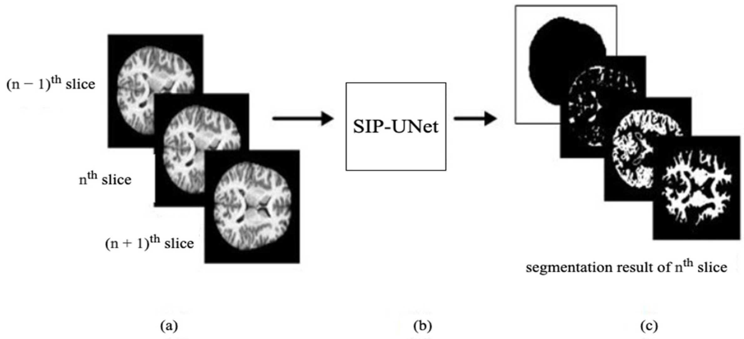
• We propose to use multiple slices as input that include neighboring slices, to extract correlated information from them.
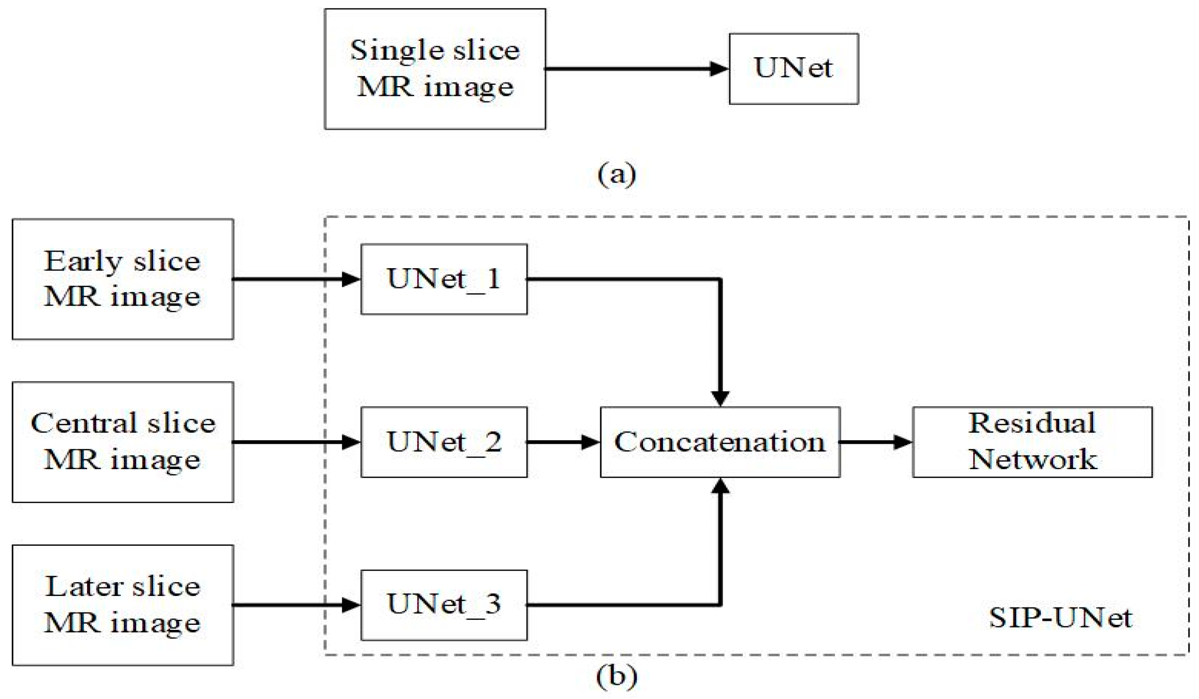
• We introduce a novel parallel UNet to preserve individual spatial information of each input slice.
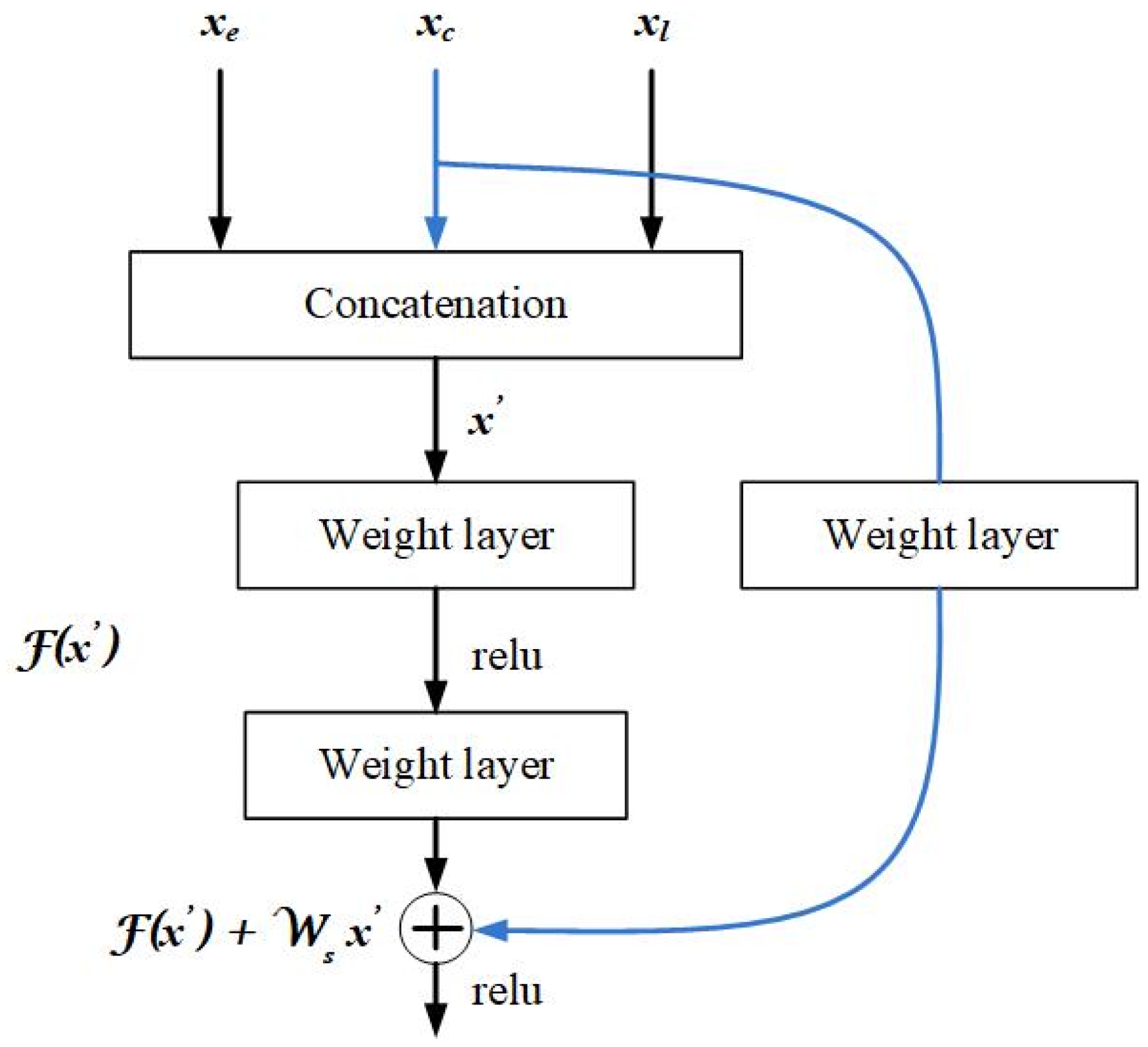
• We propose integration of the outputs of parallel Unets using a residual network with late fusion to improve the performance.
• We experiment with resizing images from OASIS data. Apart from resizing the 2D images, the proposed method does not use any augmentation, patch-wise method, pre- or post-processing of skull-stripped images.
• We also experiment with the latest state-of-the-art methods, typical UNet, and modified Unet that takes three slices. The proposed method outperforms rest of these methods.

The rest of the paper is organized as follows: Section 2.1 presents the dataset, and the evaluation criteria are shown. The proposed parallel Unet architecture is presented in detail in Section 2.2. The evaluation and the results of our novel architecture are presented in Section 3. Finally, we present discussion points, and then draw a conclusion for this work in Section 4.

2. Materials and Methods

2.1. Data

We evaluated our proposed model using the Open Access Series of Imaging Studios (OASIS) dataset [35]. There were 413 subjects and 20 non-demented subjects included in OASIS. Of the 436 subjects, we randomly selected 50 subjects for training and the remaining 386 subjects for testing the model. Each subject’s MRI scan and its segmented 3D image had dimensions of 176 × 208 × 176. We extracted 2D images for three different planes: axial, coronal, and sagittal. When converting each image to the 2D data, there were some empty images that did not contain information about the brain in all planes. We selected only slices from 15 to 145 for the axial plane, 30 to 180 slices for the coronal plane, and 25 to 145 slices for the sagittal plane to exclude empty 2D images. Because these 2D slices varied in size across different dimensions and different planes, we resized all images to the dimensions of 256 × 256. To create an input for our model, we concatenated three consecutive images after resizing them. After concatenation, the size was 256 × 256 × 3. The third dimension represented different slices instead of channels because we were using colorless images. The first slice represented the ‘early’ slice, the second slice represented the ‘central’ slice, and finally, the third slice represented the ‘late’ slice.

We used 50 subjects from the OASIS dataset for training. The same subjects were used to train the models for the different planes. From each subject, 130 2D slices (from 15 to 145) were extracted in the axial plane. Similarly, 150 2D slices (from 30 to 180) and 120 2D slices (from 25 to 145) in the coronal and sagittal planes, respectively, were extracted from each individual subject. Overall, we obtained 6500, 7500, and 6000 images from axial, coronal, and sagittal plane, respectively. While training, we used 20% of data for the validation, which gave us 1300, 1500, and 1200 images from axial, coronal, and sagittal plane, respectively, for the validation. The models were trained and tested separately for each individual plane. For testing, we used the remaining 386 subjects and extracted the images in the same way as for the training. In total, we obtained 50,180, 57,900, and 46,320 images from the axial, coronal, and sagittal planes, respectively, as test data.

2.2. Method

The ability to utilize and extract features from neighboring slices or images distinguishes SIP-UNet from typical UNet. In a typical UNet, only a single corresponding image is used as input in a typical UNet. However, in SIP-UNet two neighboring slices (‘early’ and ‘later’) are also used to obtain the segmentation result of the central slice. We visualized and compared the sequential slices. We found that the slices next to the central slice have common regions or similar structure. While comparing with the neighboring slices, the regions seemed like regions that were projected from or to the central slice. But when we considered more than three slices (5 or more), the slices that were far from the central slice by two or more slices had no common regions or structures. In some cases, they were totally different if we took slices from the lower end or upper end of the brain. Therefore, we concluded that considering more slices only increases the computational time and reduces the performance of the model. Hence, we considered only three slices, where two of them were neighboring slices. For each subject, MRI images were sliced for input data containing three consecutive slices and then jointly fed into SIP-UNet. Figure 3 shows the difference between the input for typical UNet and the proposed SIP-UNet. Figure 4 shows the architecture of conventional UNet and the one of the UNet structure used in the SIP-UNet. The proposed SIP-UNet consisted of two main parts: the parallel UNet and the late fusion using a residual network. The model was trained and tested individually for axial, sagittal, and coronal views of brain MRI.

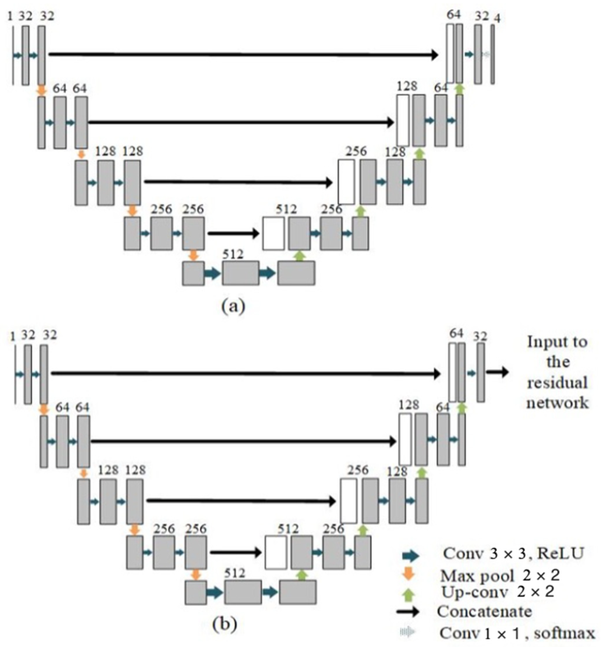
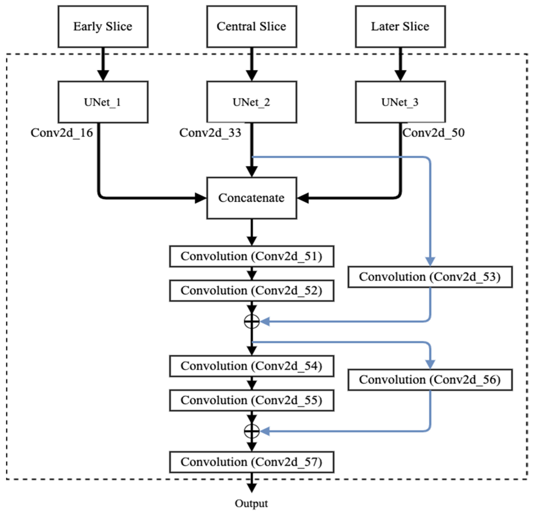
2.2.1. Parallel UNet

The parallel UNet consisted of three typical UNet that were identical to each other. Each of the slices from the input data was forwarded to a different individual UNet. The architecture of an each individual UNet that built the parallel structure in Figure 3b is shown in Figure 4b. The UNet architecture consisted of an encoder path and a decoder path. Both the encoder and decoder followed a fully convolutional network architecture. In the encoder path, a 3 × 3 convolution was repeated twice and was followed by a 2 × 2 max pooling operation that doubles the number of feature channels at each down-sampling step. Alternatively, the decoder path consisted of a 2 × 2 up-convolution that resulted in halving the number of the feature channels, followed by concatenation with the corresponding encoder path feature map and then performing two 3 × 3 convolutions. In the end, a feature map with 32 layers was obtained. Each convolutional operation in both the encoder and decoder sections was followed by a ReLU [36] activation. The structural details of typical UNet are shown in Table 1. The last convolution block which was followed by softmax function was removed in the building block of the parallel UNet. Later, the feature maps from the different UNet paths were fused using a proposed residual network.

2.2.2. Proposed Fusion Using Residual Network

In this paper, we propose a new method to combine the features of parallel UNet architectures using a residual network. First, 32 feature maps from each UNet were concatenated as shown in Figure 5. As shown in Figure 5, two 3 × 3 convolutions were performed on the concatenated feature maps as shown in Figure 5. The output of the stacked layers was then added to the central slice’s feature maps. The skip connection was used only for the feature maps of the central slice. We hypothesize that using the skip connection only for the ‘central’ slice feature maps will preserve and strengthen the information and will not let the model learn unnecessary features from the neighboring slices.

Table 1. Architecture of the single UNet.

Layer Name	Output Shape	Connected to
Input_1	256 × 256 × 1
Conv2d	256 × 256 × 32	Input_1
Conv2d_1	256 × 256 × 32	Conv2d
Max_pooling2d	128 × 128 × 32	Conv2d_1
Conv2d_2	128 × 128 × 64	Max_pooling2d
Conv2d_3	128 × 128 × 64	Conv2d_2
Max_pooling2d_1	64 × 64 × 64	Conv2d_3
Conv2d_4	64 × 64 × 128	Max_pooling2d_1
Conv2d_5	64 × 64 × 128	Conv2d_4
Max_pooling2d_2	32 × 32 × 128	Conv2d_5
Conv2d_6	32 × 32 × 256	Max_pooling2d_2
Conv2d_7	32 × 32 × 256	Conv2d_6
Max_pooling2d_3	16 × 16 × 256	Conv2d_7
Conv2d_8	16 × 16 × 512	Max_pooling2d_3
Conv2d_9	16 × 16 × 512	Conv2d_8
Conv2d_transpose	32 × 32 × 256	Conv2d_9
Concatenate	32 × 32 × 512	Conv2d_transpose, Conv2d_7
Conv2d_10	32 × 32 × 256	Concatenate
Conv2d_11	32 × 32 × 256	Conv2d_10
Conv2d_transpose_1	64 × 64 × 128	Conv2d_11
Concatenate_1	64 × 64 × 256	Conv2d_transpose_1, Conv2d_5
Conv2d_12	64 × 64 × 128	Concatenate_1
Conv2d_13	64 × 64 × 128	Conv2d_12
Conv2d_transpose_2	128 × 128 × 64	Conv2d_13
Concatenate_2	128 × 128 × 128	Conv2d_transpose_2, Conv2d_3
Conv2d_14	128 × 128 × 64	Concatenate_2
Conv2d_15	128 × 128 × 64	Conv2d_14
Conv2d_transpose_3	256 × 256 × 32	Conv2d_15
Concatenate_3	256 × 256 × 64	Conv2d_transpose_3, Conv2d_1
Conv2d_16	256 × 256 × 32	Concatenate_3
Conv2d_17	256 × 256 × 32	Conv2d_16
Conv2d_18	256 × 256 × 4	Conv2d_17

All “conv2d” corresponds to a 3 × 3 convolution block followed by ReLU activation function except for the last convolution block, which is followed by the softmax function. In case of SIP-UNet, the final convolution block is removed. Output of “Conv2d_16” is concatenated with features from same convolution layer of other two Unets; namely “Conv2d_33” and “Conv2d_50” as shown in Figure 6.

Table 1. Architecture of the single UNet.

Layer Name	Output Shape	Connected to
Input_1	256 × 256 × 1
Conv2d	256 × 256 × 32	Input_1
Conv2d_1	256 × 256 × 32	Conv2d
Max_pooling2d	128 × 128 × 32	Conv2d_1
Conv2d_2	128 × 128 × 64	Max_pooling2d
Conv2d_3	128 × 128 × 64	Conv2d_2
Max_pooling2d_1	64 × 64 × 64	Conv2d_3
Conv2d_4	64 × 64 × 128	Max_pooling2d_1
Conv2d_5	64 × 64 × 128	Conv2d_4
Max_pooling2d_2	32 × 32 × 128	Conv2d_5
Conv2d_6	32 × 32 × 256	Max_pooling2d_2
Conv2d_7	32 × 32 × 256	Conv2d_6
Max_pooling2d_3	16 × 16 × 256	Conv2d_7
Conv2d_8	16 × 16 × 512	Max_pooling2d_3
Conv2d_9	16 × 16 × 512	Conv2d_8
Conv2d_transpose	32 × 32 × 256	Conv2d_9
Concatenate	32 × 32 × 512	Conv2d_transpose, Conv2d_7
Conv2d_10	32 × 32 × 256	Concatenate
Conv2d_11	32 × 32 × 256	Conv2d_10
Conv2d_transpose_1	64 × 64 × 128	Conv2d_11
Concatenate_1	64 × 64 × 256	Conv2d_transpose_1, Conv2d_5
Conv2d_12	64 × 64 × 128	Concatenate_1
Conv2d_13	64 × 64 × 128	Conv2d_12
Conv2d_transpose_2	128 × 128 × 64	Conv2d_13
Concatenate_2	128 × 128 × 128	Conv2d_transpose_2, Conv2d_3
Conv2d_14	128 × 128 × 64	Concatenate_2
Conv2d_15	128 × 128 × 64	Conv2d_14
Conv2d_transpose_3	256 × 256 × 32	Conv2d_15
Concatenate_3	256 × 256 × 64	Conv2d_transpose_3, Conv2d_1
Conv2d_16	256 × 256 × 32	Concatenate_3
Conv2d_17	256 × 256 × 32	Conv2d_16
Conv2d_18	256 × 256 × 4	Conv2d_17

All “conv2d” corresponds to a 3 × 3 convolution block followed by ReLU activation function except for the last convolution block, which is followed by the softmax function. In case of SIP-UNet, the final convolution block is removed. Output of “Conv2d_16” is concatenated with features from same convolution layer of other two Unets; namely “Conv2d_33” and “Conv2d_50” as shown in Figure 6.

Table 2. Architecture of the proposed residual network for merging the parallel Unets.

Layer Name	Output Shape	Connected to
Concatenate_12	256 × 256 × 96	Conv2d_16, Conv2d_33, Conv2d_50
Conv2d_51	256 × 256 × 64	Concatenate_12
Conv2d_52	256 × 256 × 64	Conv2d_51
Conv2d_53	256 × 256 × 64	Conv2d_33
Add	256 × 256 × 64	Conv2d_52, Conv2d_53
Conv2d_54	256 × 256 × 32	Add
Conv2d_55	256 × 256 × 32	Conv2d_54
Conv2d_56	256 × 256 × 32	Add
Add_1	256 × 256 × 32	Conv2d_55, Conv2d_56
Conv2d_57	256 × 256 × 4	Add_1

Two convolution blocks: conv2d_51 and conv2d_54 are followed by ReLU activation function. Similarly, two addition blocks: add and add_1 are also followed by ReLU activation function. The final convolution block “conv2d_57” is followed by softmax function and generates segmented output.

Table 2. Architecture of the proposed residual network for merging the parallel Unets.

Layer Name	Output Shape	Connected to
Concatenate_12	256 × 256 × 96	Conv2d_16, Conv2d_33, Conv2d_50
Conv2d_51	256 × 256 × 64	Concatenate_12
Conv2d_52	256 × 256 × 64	Conv2d_51
Conv2d_53	256 × 256 × 64	Conv2d_33
Add	256 × 256 × 64	Conv2d_52, Conv2d_53
Conv2d_54	256 × 256 × 32	Add
Conv2d_55	256 × 256 × 32	Conv2d_54
Conv2d_56	256 × 256 × 32	Add
Add_1	256 × 256 × 32	Conv2d_55, Conv2d_56
Conv2d_57	256 × 256 × 4	Add_1

Two convolution blocks: conv2d_51 and conv2d_54 are followed by ReLU activation function. Similarly, two addition blocks: add and add_1 are also followed by ReLU activation function. The final convolution block “conv2d_57” is followed by softmax function and generates segmented output.

Formally, we denote the feature maps from ‘early’, ‘central’, and ‘later’ slices as $x_e$, $x_c$, and $x_l$ respectively, and concatenated layers as $x^{\prime }$, and let the concatenated layers fit another mapping of F$(x^{\prime })$. The underlying mapping H$\left(x^{\prime }\right)$ is defined as:

$$\mathrm{H}\left(x^{\prime }\right)=\mathrm{F}\left(x^{\prime }\right)+x_c$$

(1)

As the dimension of $x_c$ and F must be equal, a linear projection $W_s$ is performed during skip connections. The building block considered in this paper is defined as:

$$y=\mathrm{F}\left(x^{\prime },\left\{W_i\right\}\right)+W_s{x}_c$$

(2)

Here, $x^{\prime }$ and $y$ are the input and output vectors of the considered building block, respectively. The residual mapping to be learned is represented as a function F$\left(x^{\prime },\left\{W_i\right\}\right).$ In Figure 5, to omit biases for simplification of notations, we get F $=W_2\sigma \left(W_1{x}^{\prime }\right)$, where σ denotes the ReLU [36]. In this paper, the flexible residual function F has two layers. Even more layers are possible, but while using a single layer, it will be similar to a linear layer. For the linear layer: $y=W_1{x}^{\prime }+W_s{x}_c$ there are no observed advantages in the residual network [29]. Even though the notations used are generally about fully connected layers, convolutional layers can also be represented using these notations [29]. The function F$\left(x^{\prime },\left\{W_i\right\}\right)$ in Equation (2) represents convolutional layers. The structure detail of the proposed residual block is shown in Table 2. There are two skip connections in this block. The final convolution block is followed by a softmax activation function.

2.3. Loss Function

The objective of this study is to classify of brain MRI images at the pixel level. We trained our model to predict each pixel to be a member of one of the four classes. For the multi-class prediction model, we used the softmax activation function after the final convolution layer. The truth labels in our ground truth were integer encoded: 0 for background, 1 for CSF, 2 for GM, and 3 for WM. For this kind of multi-class segmentation task, the most commonly used loss function is the sparse categorical cross-entropy loss function. This cross-entropy is defined as:

$$\mathrm{L}=-\frac{1}{\left|P\right|} {{\displaystyle \sum }}_{p \in P}{y}_{i}log\left({\sigma }_i\right)$$

(3)

where ${\sigma }_i$ is the softmax probability for $i^{th}$ class for all pixels P and $y_i$ is the actual distribution. The above pixel-wise categorical cross-entropy is the total loss term. For each class, it will compute the average difference between the actual and expected probability distributions [37].

2.4. Training and Testing Schemes

Our model is for the 2D segmentation task. In our 3D medical image data, we have different views/planes: (i) axial, (ii) sagittal, and (iii) coronal. We trained the model individually for each plane and used it to make predictions and tested with it. From 3D data, we extracted 2D slices first and then concatenated three consecutive slices. From these three slices, the ‘central’ slice was predicted. Hence, we used the ground truth of the ‘central’ slice as the output for training. The input dimension for our model is 255 × 255 × 3.

We trained our SIP-UNet using the early stopping method. In the early stopping method, we used a patience value of 20. Validation data which is 20% of the training data were used to monitor the validation loss during the early stopping process. The early stopping method determines the epochs and best weight during the training. Epochs determined by the early stopping method are listed in

Table 3. Segmentation result comparison between the Multiresnet, SegNet, single-slice input UNet, multi-slice UNet, and the proposed SIP-UNet.

Axial Plane
Methods	Input Slices	Epochs	WM		GM		CSF
			DSC	JI	DSC	JI	DSC	JI
Multiresnet [21]	1	38	0.679 ± 0.180	0.538 ± 0.172	0.750 ± 0.073	0.605 ± 0.084	0.725 ± 0.079	0.574 ± 0.090
SegNet [20]	1	72	0.857 ± 0.087	0.758 ± 0.110	0.873 ± 0.050	0.778 ± 0.076	0.848 ± 0.041	0.738 ± 0.060
Unet	1	82	0.948 ± 0.075	0.908 ± 0.090	0.954 ± 0.027	0.914 ± 0.068	0.942 ± 0.032	0.893 ± 0.052
Unet (modified)	3	69	0.948 ± 0.075	0.908 ± 0.091	0.956 ± 0.027	0.917 ± 0.042	0.947 ± 0.030	0.900 ± 0.050
Proposed method	3	67	0.951 ± 0.074	0.912 ± 0.089	0.954 ± 0.026	0.923 ± 0.041	0.951 ± 0.074	0.912 ± 0.089
Coronal plane
Multiresnet [21]	1	50	0.737 ± 0.090	0.590 ± 0.101	0.762 ± 0.050	0.617 ± 0.063	0.736 ± 0.056	0.585 ± 0.068
SegNet [20]	1	70	0.889 ± 0.048	0.803 ± 0.073	0.886 ± 0.032	0.796 ± 0.049	0.861 ± 0.039	0.758 ± 0.058
Unet	1	64	0.959 ± 0.027	0.924 ± 0.044	0.954 ± 0.022	0.912 ± 0.035	0.941 ± 0.031	0.881 ± 0.049
Unet (modified)	3	101	0.962 ± 0.028	0.928 ± 0.046	0.958 ± 0.022	0.919 ± 0.036	0.948 ± 0.030	0.902 ± 0.048
Proposed method	3	82	0.962 ± 0.027	0.928 ± 0.044	0.959 ± 0.022	0.921 ± 0.035	0.951 ± 0.028	0.907 ± 0.046
Sagittal plane
Multiresnet [21]	1	42	0.720 ± 0.127	0.576 ± 0.134	0.761 ± 0.041	0.616 ± 0.050	0.738 ± 0.049	0.587 ± 0.060
SegNet [20]	1	73	0.830 ± 0.086	0.748 ± 0.118	0.868 ± 0.035	0.769 ± 0.053	0.845 ± 0.037	0.733 ± 0.054
Unet	1	78	0.951 ± 0.038	0.909 ± 0.060	0.954 ± 0.022	0.912 ± 0.035	0.944 ± 0.027	0.894 ± 0.043
Unet (modified)	3	102	0.954 ± 0.040	0.915 ± 0.062	0.957 ± 0.022	0.919 ± 0.036	0.949 ± 0.028	0.903 ± 0.044
Proposed method	3	75	0.955 ± 0.038	0.916 ± 0.060	0.959 ± 0.021	0.921 ± 0.034	0.953 ± 0.026	0.911 ± 0.041

The training epochs mentioned in the table are not defined manually. We used early stopping features of the Keras library to determine the eochs.

for all training processes. We want our model to predict all the slices of the brain. We fed all slices of each training subject into the model, except for the slices that did not contain any brain parts. The selection of these concatenated slices for training was random. First, all the valid slices (containing brain information/parts) of the training subject were converted into the desired shape and stored in a training folder in NumPy array format. A random selection from this data, with batch size of five, was used for training purposes.

During testing, the plane corresponding to the training plane was extracted and predicted. For example, if we trained a model using an axial plane, the data related to the axial plane were tested. Similar to the training data, the test input consisted of three consecutive 2D slices and was fed to the model. The ground truth of the ‘central’ slice was also stored, which was later used to evaluate the model by comparing it with the result.

2.5. Evaluation Metrices

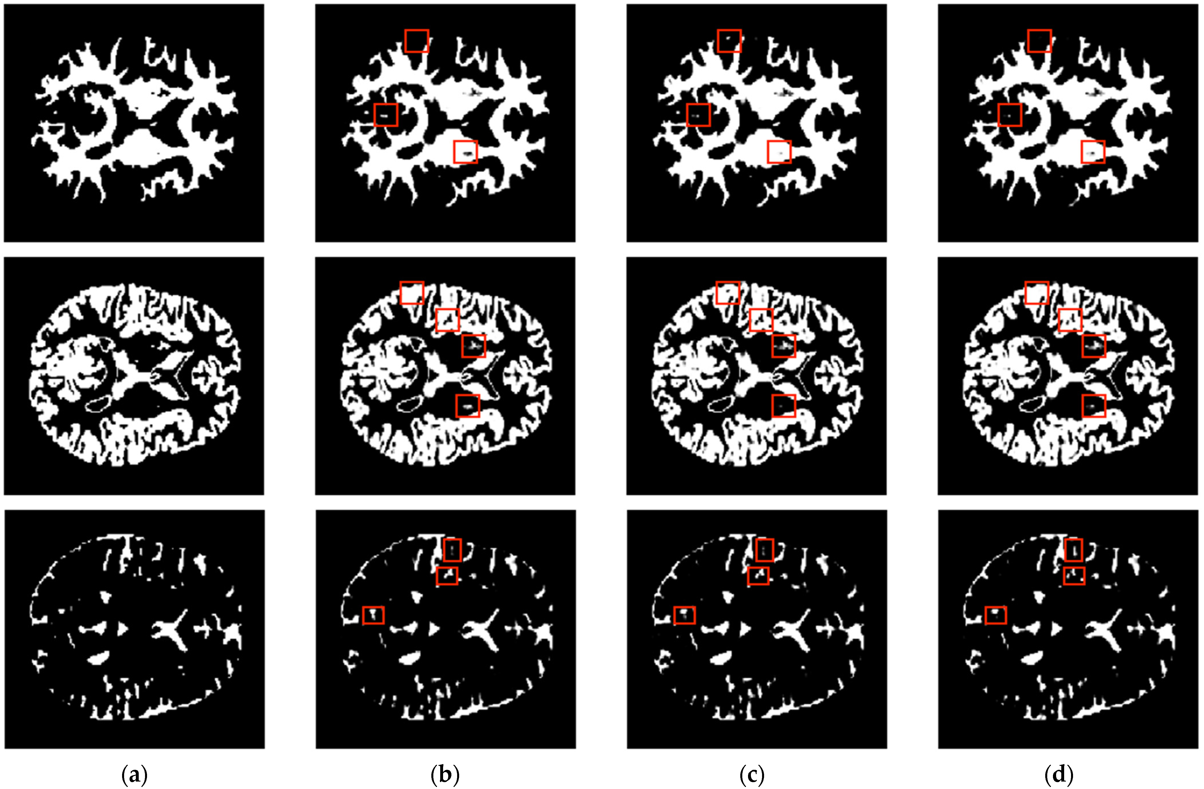
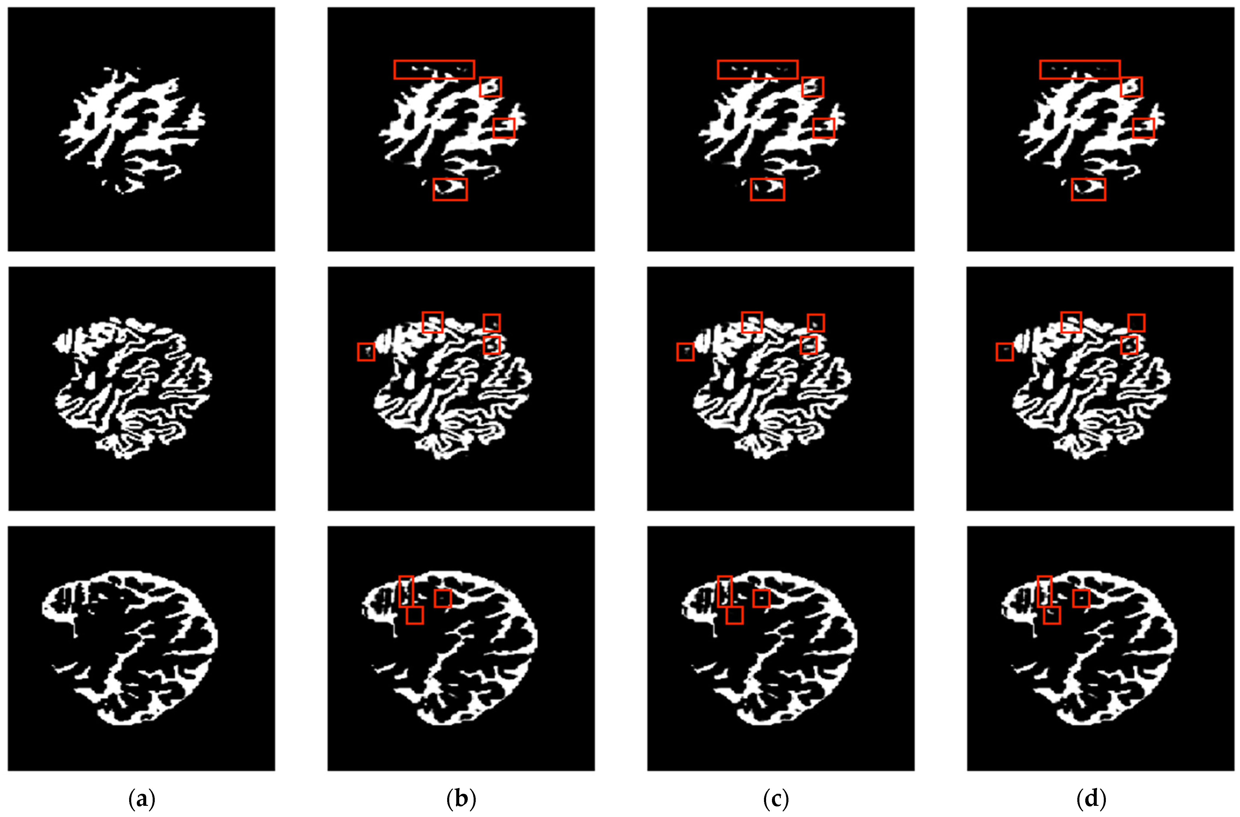
For the performance evaluation, we used the Dice Similarity Coefficient (DSC), the Jaccard Index (JI), Volumetric Overlap Error (VOE) [38], and Relative Volume Difference (RVD) [39]. The JI is the ratio of the overlapping area between the predicted and the ground-truth images to the union area between them. Another metric, the DSC is the ratio of two times the overlapping area between ground truth and the predicted images to the total number of pixels. The VOE is the ratio between intersection and union of the predicted and the ground truth images. Similarly, the RVD gives us the absolute size difference of the images, as a fraction of the size of the reference.

For the ground truth segmentation map $I$ and the predicted segmentation map $I^{\prime }$, the JI and the DSC are defined in Equations (4) and (5), respectively.

$$JI=\frac{\left|I\cap I^{\prime }\right|}{\left|I\cup I^{\prime }\right|}$$

(4)

$$DSC=\frac{2\left|I\cap I^{\prime }\right|}{\left|I\right|+\left|I^{\prime }\right|}$$

(5)

$$VOE=1-\frac{\left|I\cap I^{\prime }\right|}{\left|I\cup I^{\prime }\right|}$$

(6)

$$RVD=\pm \frac{\left|I\right|-\left|I^{\prime }\right|}{\left|I\right|}$$

(7)

Because there are four classes in our segmentation, the JI and the DSC were calculated for each class separately. Among the four classes, performance on the background segmentation was not evaluated. The background segmentation can also be performed with simpler models. We compared the performance of the models for the remaining three classes: CSF, GM, and WM. In multi-class segmentation, the evaluation metrics were calculated for each class separately. For example, if we wanted to calculate the JI for CSF, then pixels related to CSF were assigned to the value of 1, and the value of 0 was assigned to the rest of the pixels. The same procedure was followed for GM and WM.

3. Results

In Section 3.1, we perform a study based on the input of a single slice and multiple slices in a simple UNet model and show the improvement by using SIP-UNet in segmentation. We then evaluate and compare the segmentation performance with various current models in Section 3.2.

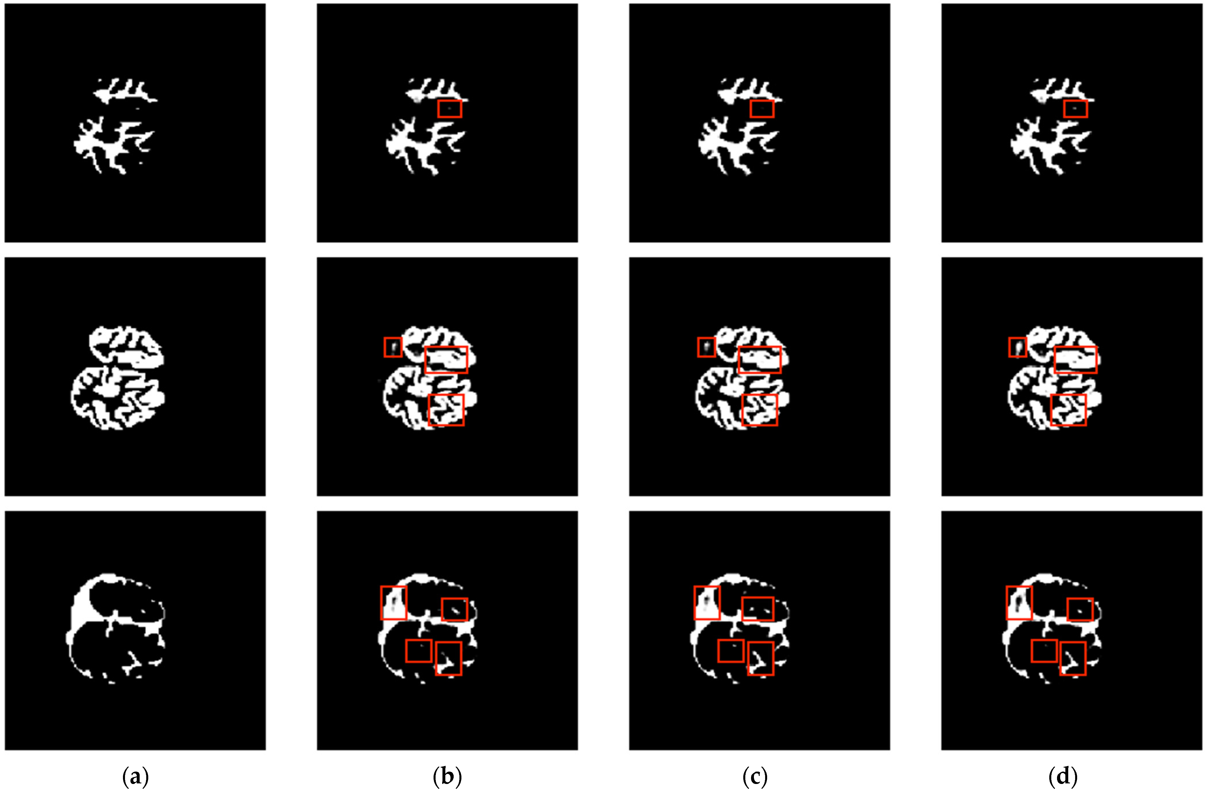
3.1. Analysis and Comparison with Single-Slice and Multiple-Slice Input UNet

UNet has better performance in segmenting biomedical images. We first tested the UNet with a single-slice input for segmentation. The investigation purpose of testing with a single-slice input was to compare it with the multi-slices input to see whether the results are better with or without the neighboring slice’s features. Later the same UNet was modified in the input layer to make it suitable for processing inputs containing neighboring slices. The input in this UNet contained three 2D planes. The planes comprised the neighboring slices.

Most of the previous studies [10,14,40] used only a certain number of slices. In [14,40], the slices were selected alternately or only one slice was selected from a few slices. The purpose of predicting and training only a selected number of slices was to avoid repeating information from the neighboring slices since the 2D slices are similar to each other. However, these methods are insufficient to quantify changes in the brain because they do not consider the entire set of brain. In this study, we have included all of the slices that comprise parts of the brain. This helps in quantifying changes in each layer and will later lead to matching results in the 3D quantification.

The evaluation of UNet with single and multiple slices with the proposed SIP-UNet is shown in Table 3 based on the DSC and the JI scores. The scores are average scores from the test images of the corresponding plane. From the table, it can be observed that the DSC score in the SIP-UNet is slightly improved for the single-slice and multi-slice UNet. Considering only the axial plane, the DSC score using simple UNet is 0.948, 0.954, and 0.942 for WM, GM, and CSF, respectively, whereas the DSC scores obtained using the SIP-UNet are 0.951, 0.954, and 0.951 for WM, GM, and CSF, respectively. The UNet with single input has an almost identical DSC score as the UNet with multi-slices input. From the Table 3, we can see that the DSC score of WM and CSF in axial plane is higher than the UNet and multi-slice UNet. Moreover, the JI score for all tissues in the axial plane is higher than the other two UNets. In the coronal plane, the JI score of the GM and the DSC score of the CSF are higher than other two models. Moreover, in sagittal plane, the JI score of both GM and CSF along with the DSC score of the CSF is higher than the UNet and multi-slice input UNet. Our proposed model has higher scores in the case of CSF than the other UNets. CSF is a colorless liquid. It is very difficult to segment. But our proposed model performed better in case of CSF. With higher scores for CSF in all three planes, higher DSC and JI scores for WM in axial plane, and finally higher JI scores for GM in all three planes, our model outperformed typical UNet and the multi-slice input UNet.

To investigate the improvement in the result of the SIP-UNet result, we visually compared the results of specific slices of a random subject. The comparison of the specific tissue segmentation was easier with the binary mapping of the corresponding tissue. We created a binary map of WM, GM, and CSF separately and then compared it with the results of the different models and the ground truth. Figure 7 shows the result for the axial plane. The column represents the ground truth and the results of the following: the one slice input UNet, the multi-slice input UNet, and the proposed SIP-UNet respectively. The row represents a binary map of the different tissues: WM, GM, and CSF from top to bottom. The binary map shown in Figure 7 is a 70th slice in the axial plane from the randomly selected subject. The difference observed in the pattern of the binary map of the different models is highlighted with a red box in the figures. In the first row of WM, the binary map of the multi- slice UNet output has a false prediction in a region highlighted by the red box at the top of the image. However, there is no such false prediction in the other two models. In the same row, the box in the middle shows the false prediction in all of the three models’ outputs. In this case, in the ground truth, there is no such tissue in the area covered by the middle red box, but we can see the false prediction in all of the outputs. However, if we analyze it and take a clear look at it, we can see that the area of the false predicted tissue in the middlebox in the SIP-UNet result is much smaller. Thus, even in the region of the false prediction, the result of the proposed SIP-UNet is closer to the ground truth than the other two models. The last red box from the top in the first row shows the region where the single-slice UNet failed to predict the presence of tissue in that region, whereas the other two models were successful. Among the three highlighted regions in the first row, the proposed SIP-UNet gives a result closer to the ground truth.

The second row of Figure 7 compares the binary map of GM. The first highlighted area shows the region where the multi-slices input UNet has predicted false. In the remaining three highlighted regions, all of the three models were successful but the shape and edge of the predicted result in these regions differ in the single-slice and multi-slice input UNet. The proper edge and area of the tissues in these regions are correct with the proposed SIP-UNet model. The third row contains the results for the CSF. Similar to GM in the second row, the single-slice and multi-slice UNet models predicted the tissues in the highlighted regions but could not provide the result with the same area and edge as in the ground truth. In contrast, the SIP-UNet predicted the tissues in this region with an edge and shape similar to the ground truth.

Figure 8 shows the segmentation results for the coronal plane. The subject was randomly chosen and the 30th slice in the coronal plane of this subject segmented with different models is presented in columns. The first row contains the WM binary map, where we can see that the result of SIP-UNet (last column) is able to predict a very small region consisting of WM, whereas the rest of the other two UNets with a single-slice and multi-slice are unable to predict this part. From the lower two rows of GM and CSF, a region is highlighted in the top left corner that was incorrectly predicted. This misprediction in GM resulted in no CSF in that region as shown in the last row. However, this misclassification appeared in all three models. Although the proposed model is not perfect, we can see the improvement in the remaining highlighted regions. In the remaining highlighted regions, the single-slice and multi-slice UNets are unable to predict the presence of smaller tissues. The two highlighted regions to the right of the GM predicted results (second row) show that the classical UNet cannot detect smaller details. However, the SIP-UNet performed well in these smaller regions and also maintained the edges of the tissues close to the ground truth.

Similar to the axial and coronal planes, the SIP-UNet also performed better in the sagittal plane. In Figure 9, the segmented results of the different models are arranged in different columns and the rows represent the different tissues as before. We can see the miss prediction of tissue segmentation in the top highlighted region in the first row (WM binary map). All models have the wrong segmented output in this region, but if we look closely, the segmented WM in this region is comparatively lower in the result of SIP-UNet, so it is close to the ground truth. The bottom highlighted region in the first row shows how well the edge is predicted in the SIP-UNet. The same region in the multi-slice input UNet has disconnected tissue, while the SIP-UNet has a region that is close to the ground truth. Similarly, in the top left highlighted region in the last row (CSF binary map) of Figure 9, both the single-slice and multi-slice input UNet has disconnected tissue, whereas the SIP-UNet result has a connected tissue that matches the ground truth. In the rest of the highlighted regions in the second and third rows in Figure 9, we can see how well the SIP-UNet performs in the regions where the typical UNet fails. In summary, the proposed architecture can extract smaller details and edges of the tissue than the other implemented models and the typical UNets. Although the DSC scores of the typical UNets are almost identical to those of the proposed methods, the JI score of the proposed method is increased, indicating better performance.

3.2. Comparisons with Other Methods

Table 3 compares the performance of Multiresnet (Available online: https://github.com/nibtehaz/MultiResUNet/blob/master/MultiResUNet.py, accessed on 14 December 2021), SegNet (Available online: https://github.com/divamgupta/image-segmentation-keras/blob/master/keras_segmentation/models/segnet.py, accessed on 20 December 2021), the typical UNet, and the proposed UNet on the same dataset. We implemented all the models listed in Table 1 and trained and tested them on the same data. In this table, we implement Multiresnet and SegNet using the code available on GitHub. The multi-slice input UNet is the modification of the single-slice input UNet, where the input layer of the model is changed from one 2D input at a time to three 2D inputs simultaneously.

In terms of the DSC score, the proposed model has the highest mean score compared to Multiresnet and SegNet. The DSC score of the proposed method is between 95% and 96% for all three classes in all planes. Our goal is to extract information from the neighboring slices without data augmentations and without any additional pre- or post-processing other than resizing the image to fit in the model. Without any additional processing, the Multiresnet only achieved a DSC score between 67% and 76%, and SegNet achieved an average DSC value between 83% and 88%. All the models listed in Table 3 have a lower DSC value than the proposed method. Additionally, the JI score of the proposed method is the highest among the implemented Multiresnet and SegNet. The average JI score of the proposed method is in the range of 90% to 92% whereas the average JI score of Multiresnet is in the range of 53% to 61% and that of SegNet is in the range of 73% to 80%. In the implemented models, the output for all slices of the brain and all three planes has a lower performance for both evaluation matrices. This indicates that the proposed model is significantly better.

In

Table 4. RVD and VOE comparison between the Multiresnet, SegNet, single-slice input UNet, multi-slice UNet, and the proposed SIP-UNet.

Axial Plane
Methods	Input Slices	Epochs	WM		GM		CSF
			RVD(%)	VOE	RVD(%)	VOE	RVD(%)	VOE
Multiresnet [21]	1	38	−14.362	0.462	−4.692	0.395	−5.935	0.426
SegNet [20]	1	72	2.468	0.242	−2.618	0.222	3.129	0.262
Unet	1	82	2.261	0.092	−0.4114	0.086	0.4507	0.107
Unet (modified)	3	69	2.214	0.092	0.3998	0.083	−1.073	0.100
Proposed method	3	67	0.4833	0.088	−0.2854	0.077	0.9819	0.088
Coronal plane
Multiresnet [21]	1	50	−8.48	0.41	−3.429	0.383	−1.648	0.415
SegNet [20]	1	70	−0.0132	0.197	−1.647	0.204	4.21	0.242
Unet	1	64	−0.0583	0.076	−1.148	0.088	2.149	0.119
Unet (modified)	3	101	0.544	0.072	−1.072	0.081	1.49	0.098
Proposed method	3	82	−0.009	0.072	−0.548	0.079	0.881	0.093
Sagittal plane
Multiresnet [21]	1	42	−10.46	0.424	−0.724	0.384	−4.511	0.413
SegNet [20]	1	73	−0.665	0.252	−1.132	0.231	1.297	0.267
Unet	1	78	1.978	0.091	−0.669	0.088	−0.337	0.106
Unet (modified)	3	102	−0.779	0.085	−0.4686	0.081	1.547	0.097
Proposed method	3	75	−1.228	0.084	0.5545	0.079	−0.3729	0.089

, we compared the VOE and RVD scores of the models for the different planes. The RVD scores are given in percentage, which means the scores are multiplied by 100 because the scores were too small to be shown in the table. From the table, the VOE of the proposed method is less than the other methods for tissues in all planes, which means the error is less in the proposed method. In case of the RVD scores, the scores in percentage are also smaller with respect to the rest of the model. This helps to interpret that the output of the proposed model has relatively less difference volume than the ground truth. Hence, from the VOE and the RVD scores, we can conclude that the result of the proposed method is close to the ground truth and performs better than the other models.

We would like to mention that all the results used for comparison in

Table 5. Comparison of different approaches for brain structure segmentation.

Authors	Methods	DSC Score
		WM	GM	CSF
Zhang et al. [43]	CNN	86.4%	85.2%	83.5%
Nie et al. [34]	FCN	88.7%	87.3%	85.5%
Khagi et al. [10]	SegNet	81.9%	74.6%	72.2%
Lee et al. [41]	Patch-wise UNet	94.33%	93.33%	92.67%
Yamanakkanavar et al. [42]	Patch-wise Mnet	95.17%	94.32%	93.60%
Proposed method	SIP-UNet	95.6%	95.73%	95.2%

for comparison are directly used from the published papers. We have not implemented four of the methods in this table. In Table 5, three of the methods (CNN, FCN, and SegNet) are obtained from Khagi et al. [10]. The result of patch-wise UNet is obtained from Lee et al. [41]. The DSC score for each tissue is in Lee et al. [41] and the proposed method is calculated using the average score of the three different planes for the corresponding tissue. The scores for the patch-wise Mnet are taken directly from Yamanakkanavar et al. [42].

From Table 5, it can be seen that the UNet-based deep learning architectures outperform other segmentation models. In terms of the DSC score, the proposed SIP-UNet has the highest mean score of 95.6%, 95.73%, and 95.2% for the WM, GM, and CSF, respectively. The performance of patch-wise UNet is higher than other methods and is close to the proposed method. But according to Lee et al. [41], only slices with an interval of three are used, which includes 48 slices per subject. The result for all of the slices using the patch-wise method is unknown, and although only 48 slices per subject were used in that paper, the DSC score is lower than the proposed method. Similar to the patch-wise UNet method, another method using patch-wise Mnet also uses 48 slices per subjects. All the deep learning-based methods have relatively lower DSC scores than the UNet-based deep learning architectures. In summary, the proposed strategy can achieve significantly higher segmentation performance for all three planes regardless of the number of slices and the selected plane.

4. Discussion and Conclusions

Brain tissue segmentation plays a crucial role in quantifying changes in the brain. In this work, we presented a fully automated brain tissue segmentation method that uses the neighboring slices to extract correlated information.

In contrast to typical deep learning models where only one slice serves as the input, the proposed SIP-UNet benefits from neighboring slices by extracting additional information from them. SIP-UNet can achieve a better segmentation result for axial, coronal, and sagittal 2D planes. Both qualitative analysis by visual comparison and quantitative analysis indicate that our segmentations are reliable. The proposed method can significantly improve the performance in all three planes, and the average DSC and JI scores outperform the existing deep learning-based segmentation models. The average DSC scores for the testing OASIS dataset was 95.6%, 95.73%, and 95.2% for the WM, GM, and CSF respectively. Similarly, the average JI scores for the testing OASIS dataset were 91.87%, 92.16%, and 91.00% for WM, GM, and CSF respectively. The proposed method achieved a comparatively better JI score than the typical UNets. The CSF is a colorless liquid, and it is very difficult to segment it in medical imaging. Most of the methods and models perform poor in the case of CSF. But the proposed model is better than the typical UNet in the case of segmenting CSF. However, in terms of the DSC score, the proposed method is comparable to others and there is still room for improvement.

To prepare 2D data for training and testing, we extracted 2D slices for each plane separately and then stacked the neighboring slices on the top and at the bottom of the middle slice that was to be predicted. The evaluation matrix was computed from the average of the scores since we wanted to compare the performance of the model regardless of the subject and the number of slices.

Our goal was to extract information from the neighboring slices for improvement. Our model consisted of parallel UNets that were later merged with a residual network. The purpose of this approach was to extract features from each slice separately without mixing or suppressing the features of the middle/current slice. From the scores of the evaluation matrix and visual comparison of the results, we can conclude that the model has succeeded in extracting features from neighboring slices, which leads to an improvement in the segmentation result. The proposed method was comparatively successful in extracting minute details about the edges and detecting smaller tissue regions.

Since most MRI brain data is in 3D and includes multiple slices, this method can be extended to other tasks related to segmentation. In the case of videos, a 2D frame also has neighboring slices. If the video data has a high number of frames per second, then the successive frames have similar information that can improve results. The proposed method can also be useful for other segmentation works such as in video data.

A potential limitation of this work is that the proposed model requires more memory and computation time than the typical UNet. But the proposed method has shown promising segmentation performance. In our future work, we will modify the UNet used in parallel to improve the computational efficiency of the proposed SIP-UNet architecture. In addition, we aim to further improve the segmentation performance by using a different approach to merge the features from the parallel UNets. A possible solution is to increase the skip connections and create a deeper residual network for merging the features from the parallel UNets.

References

1. Badrinarayanan, V.; Kendall, A.; Cipolla, R. SegNet: A Deep Convolutional Encoder-Decoder Architecture for Image Segmentation. IEEE Trans. Pattern Anal. Mach. Intell. 2017, 39, 2481–2495. [Google Scholar] [CrossRef] [PubMed]
2. Bauer, S.; Wiest, R.; Nolte, L.; Reyes, M. A survey of MRI-based medical image analysis for brain tumor studies. Phys. Med. Biol. 2013, 58, R97–R129. [Google Scholar] [CrossRef] [Green Version]
3. Hsiao, C.J.; Hing, E.; Ashman, J. Trends in Electronic Health Record System Use Among Office-based Physicians: United States, 2007–2012. Natl. Health Stat. Rep. 2014, 1, 1–18. [Google Scholar]
4. Despotović, I.; Goossens, B.; Philips, W. MRI segmentation of the human brain: Challenges, methods, and applications. Comput. Math. Methods Med. 2015, 2015, 450341. [Google Scholar] [CrossRef] [Green Version]
5. Ulku, I.; Akagunduz, E. A Survey on Deep Learning-based Architectures for Semantic Segmentation on 2D images. arXiv 2019, arXiv:1912.10230. [Google Scholar] [CrossRef]
6. Lafferty, J.; McCalium, A.; Pereira, F.C. Conditional Random Fields: Probabilistic Models for Segmenting and Labeling Sequence Data. In Proceedings of the Eighteenth International Conference on Machine Learning, Williamstown, MA, USA, 28 June–1 July 2001; pp. 282–289. [Google Scholar]
7. Ganin, Y.; Lempitsky, V. N4-Fields: Neural Network Nearest Neighbor Fields for Image Transforms. arXiv 2014, arXiv:1406.6558. [Google Scholar]
8. Ning, F.; Delhomme, D.; LeCun, Y.; Piano, F.; Bottou, L.; Barbano, P.E. Toward automatic phenotyping of developing embryos from videos. IEEE Trans. Image Process. 2005, 14, 1360–1371. [Google Scholar] [CrossRef] [PubMed] [Green Version]
9. Ibtehaz, N.; Sohel Rahman, M. MultiResUNet: Rethinking the U-Net Architecture for Multimodal Biomedical Image Segmentation. arXiv 2019, arXiv:1902.04049. [Google Scholar] [CrossRef]
10. Khagi, B.; Kwon, G.R. Pixel-Label-Based Segmentation of Cross-Sectional Brain MRI Using Simplified SegNet Architecture-Based CNN. J. Healthc. Eng. 2018, 2018, 3640705. [Google Scholar] [CrossRef] [PubMed] [Green Version]
11. Gu, Z.; Cheng, J.; Fu, H.; Zhou, K.; Hao, H.; Zhao, Y.; Zhang, T.; Gao, S.; Liu, J. CE-Net: Context Encoder Network for 2D Medical Image Segmentation. IEEE Trans. Med. Imaging 2019, 38, 2281–2292. [Google Scholar] [CrossRef] [Green Version]
12. Long, J.; Shelhamer, E.; Darrell, T. Fully Convolutional Networks for Semantic Segmentation. arXiv 2014, arXiv:1411.4038. [Google Scholar]
13. Ronneberger, O.; Fischer, P.; Brox, T. U-Net: Convolutional Networks for Biomedical Image Segmentation. arXiv 2015, arXiv:1505.04597. [Google Scholar]
14. Yamanakkanavar, N.; Choi, J.; Lee, B. MRI Segmentation and Classification of Human Brain Using Deep Learning for Diagnosis of Alzheimer’s Disease: A Survey. Sensors 2020, 20, 3243. [Google Scholar] [CrossRef] [PubMed]
15. Punn, S.N.; Agarwal, S. Modality specific U-Net variants for biomedical image segmentation: A survey. arXiv 2021, arXiv:2107.04537. [Google Scholar] [CrossRef] [PubMed]
16. Zhang, B.; Mu, H.; Gao, M.; Ni, H.; Chen, J.; Yang, H.; Qi, D. A Novel Multi-Scale Attention PFE-UNet for Forest Image Segmentation. Forests 2021, 12, 937. [Google Scholar] [CrossRef]
17. Rehman, M.U.; Cho, S.; Kim, J.H.; Chong, K.T. BU-Net: Brain Tumor Segmentation Using Modified U-Net Architecture. Electronics 2020, 9, 2203. [Google Scholar] [CrossRef]
18. Comelli, A.; Dahiya, N.; Stefano, A.; Vernuccio, F.; Portoghese, M.; Cutaia, G.; Bruno, A.; Salvaggio, G.; Yezzi, A. Deep Learning-Based Methods for Prostate Segmentation in Magnetic Resonance Imaging. Appl. Sci. 2021, 11, 782. [Google Scholar] [CrossRef] [PubMed]
19. Gadosey, P.K.; Li, Y.; Agyekum, E.A.; Zhang, T.; Liu, Z.; Yamak, P.T.; Essaf, F. SD-UNet: Stripping down U-Net for Segmentation of Biomedical Images on Platforms with Low Computational Budgets. Diagnostics 2020, 10, 110. [Google Scholar] [CrossRef] [PubMed] [Green Version]
20. Isensee, F.; Petersen, J.; Klein, A.; Zimmerer, D.; Jaeger, P.F.; Kohl, S.; Wasserthal, J.; Koehler, G.; Norajitra, T.; Wirkert, S.; et al. nnU-Net: Self-adapting Framework for U-Net-Based Medical Image Segmentation. arXiv 2018, arXiv:1809.10486. [Google Scholar]
21. Blanc-Durand, P.; Gucht, A.V.D.; Schaefer, N.; Itti, E.; Prior, J.O. Automatic lesion detection and segmentation of 18F-FET PET in gliomas: A full 3D U-Net convolutional neural network study. PLoS ONE 2018, 13, e0195798. [Google Scholar] [CrossRef] [PubMed]
22. Tong, G.; Li, Y.; Chen, H.; Zhang, Q.; Jiang, H. Improved U-NET network for pulmonary nodules segmentation. Optik 2018, 174, 460–469. [Google Scholar] [CrossRef]
23. Dong, H.; Yang, G.; Liu, F.; Mo, Y.; Guo, Y. Automatic Brain Tumor Detection and Segmentation Using U-Net Based Fully Convolutional Networks. arXiv 2017, arXiv:1705.03820. [Google Scholar]
24. Que, Q.; Tang, Z.; Wang, R.; Zeng, Z.; Wang, J.; Chua, M.; Sin Gee, T.; Yang, X.; Veeravalli, B. CardioXNet: Automated Detection for Cardiomegaly Based on Deep Learning. In Proceedings of the 2018 40th Annual International Conference of the IEEE Engineering in Medicine and Biology Society (EMBC), Honolulu, HI, USA, 18–21 July 2018; pp. 612–615. [Google Scholar]
25. Zhang, Y.; Wu, J.; Liu, Y.; Chen, Y.; Wu, E.X.; Tang, X. MI-UNet: Multi-Inputs UNet Incorporating Brain Parcellation for Stroke Lesion Segmentation From T1-Weighted Magnetic Resonance Images. IEEE J. Biomed. Health Inform. 2021, 25, 526–535. [Google Scholar] [CrossRef]
26. Kong, Y.; Li, H.; Ren, Y.; Genchev, G.Z.; Wang, X.; Zhao, H.; Xie, Z.; Lu, H. Automated yeast cells segmentation and counting using a parallel U-Net based two-stage framework. OSA Continuum 2020, 3, 982–992. [Google Scholar] [CrossRef]
27. Dolz, J.; Ben Ayed, I.; Desrosiers, C. Dense Multi-path U-Net for Ischemic Stroke Lesion Segmentation in Multiple Image Modalities. arXiv 2018, arXiv:1810.07003. [Google Scholar]
28. Tran, S.T.; Cheng, C.H.; Nguyen, T.T.; Le, M.H.; Liu, D.G. TMD-Unet: Triple-Unet with Multi-Scale Input Features and Dense Skip Connection for Medical Image Segmentation. Healthcare 2021, 9, 54. [Google Scholar] [CrossRef]
29. He, K.; Zhang, X.; Ren, S.; Sun, J. Deep Residual Learning for Image Recognition. In Proceedings of the 2016 IEEE Conference on Computer Vision and Pattern Recognition (CVPR), Las Vegas, NV, USA, 27–30 June 2016; pp. 770–778. [Google Scholar]
30. Diakogiannis, F.I.; Waldner, F.; Caccetta, P.; Wu, C. ResUNet-a: A deep learning framework for semantic segmentation of remotely sensed data. ISPRS J. Photogramm. Remote Sens. 2020, 162, 94–114. [Google Scholar] [CrossRef] [Green Version]
31. Liu, H.; Jiang, J. U-Net Based Multi-instance Video Object Segmentation. arXiv 2019, arXiv:1905.07826. [Google Scholar]
32. Perazzi, F.; Khoreva, A.; Benenson, R.; Schiele, B.; Sorkine-Hornung, A. Learning Video Object Segmentation from Static Images. In Proceedings of the 2017 IEEE Conference on Computer Vision and Pattern Recognition (CVPR), Honolulu, HI, USA, 21–26 July 2017; pp. 3491–3500. [Google Scholar]
33. Vu, M.; Grimbergen, G.; Nyholm, T.; Löfstedt, T. Evaluation of multislice inputs to convolutional neural networks for medical image segmentation. Med. Phys. 2020, 47, 6216–6231. [Google Scholar] [CrossRef] [PubMed]
34. Nie, D.; Wang, L.; Gao, Y.; Shen, D. Fully convolutional networks for multi-modality isointense infant brain image segmentation. In Proceedings of the 2016 IEEE 13th International Symposium on Biomedical Imaging (ISBI), Prague, Czech Republic, 13–16 April 2016; pp. 1342–1345. [Google Scholar]
35. Marcus, D.S.; Wang, T.H.; Parker, J.; Csernansky, J.G.; Morris, J.C.; Buckner, R.L. Open Access Series of Imaging Studies (OASIS): Cross-sectional MRI data in young, middle aged, nondemented, and demented older adults. J. Cogn. Neurosci. 2007, 19, 1498–1507. [Google Scholar] [CrossRef] [Green Version]
36. Nair, V.; Hinton, G. Rectified Linear Units Improve Restricted Boltzmann Machines. ICML 2010, 27, 807–814. [Google Scholar]
37. Rohlfing, T. Image Similarity and Tissue Overlaps as Surrogates for Image Registration Accuracy: Widely Used but Unreliable. IEEE Trans. Med. Imaging 2021, 31, 153–163. [Google Scholar] [CrossRef] [PubMed] [Green Version]
38. Powers, D.M. Evaluation: From precision, recall and F-measure to ROC, informedness, markedness and correlation. arXiv 2020, arXiv:2010.16061. [Google Scholar]
39. Yeghiazaryan, V.; Voiculescu, I.D. Family of boundary overlap metrics for the evaluation of medical image segmentation. J. Med. Imaging 2018, 5, 015006. [Google Scholar] [CrossRef] [PubMed]
40. Yamanakkanavar, N.; Lee, B. A novel M-SegNet with global attention CNN architecture for automatic segmentation of brain MRI. Comput. Biol. Med. 2021, 136, 104761. [Google Scholar] [CrossRef] [PubMed]
41. Lee, B.; Yamanakkanavar, N.; Choi, J. Automatic segmentation of brain MRI using a novel patch-wise U-net deep architecture. PLoS ONE 2020, 15, e0236493. [Google Scholar] [CrossRef] [PubMed]
42. Yamanakkanavar, N.; Lee, B. Brain Tissue Segmentation using Patch-wise M-net Convolutional Neural Network. In Proceedings of the 2020 IEEE International Conference on Consumer Electronics—Asia (ICCE-Asia), Seoul, Korea, 1–3 November 2020; pp. 1–4. [Google Scholar]
43. Zhang, W.; Li, R.; Deng, H.; Wang, L.; Lin, W.; Ji, S.; Shen, D. Deep convolutional neural networks for multi-modality isointense infant brain image segmentation. NeuroImage 2015, 108, 214–224. [Google Scholar] [CrossRef] [Green Version]
Figure 1. Binary map of four different classes generated from ground truth.
Mathematics 10 02755 g001
Figure 2. Illustration of SIP-UNet (a) input comprises three consecutive slices where (n – 1)th slice represents the early slice, nth slice represents the central slice, and (n + 1)th slice represents the later slice, (b) the proposed SIP-UNet model, and (c) output of the proposed model which generates the segmented result of nth slice.
Mathematics 10 02755 g002
Figure 3. Illustration of procedure for: (a) typical UNet and (b) proposed SIP-UNet.
Mathematics 10 02755 g003
Figure 4. Architecture of single UNet for: (a) typical conventional segmentation and (b) one of the three parallel Unets which encodes and decodes one of the three slices in SIP-UNet.
Mathematics 10 02755 g004
Figure 5. The proposed building block of residual learning for merging the three parallel Unets. x e denotes output features from the UNet for the early slice, x l denotes output features from the UNet for the later slice, and x c denotes output from UNet for the central slice, which is used in the skip connection for residual learning.
Mathematics 10 02755 g005
Figure 6. Illustration of the proposed network for the fusion of the filters from parallel Unets. The corresponding layer names that are input for the concatenation are from the Table 2. The output features of Conv2d_16, Conv2d_33, and Conv2d_50 are the input for the concatenation before the residual network as shown in the figure.
Mathematics 10 02755 g006
Figure 7. Illustration of segmentation results for axial plane for existing methods and SIP-UNet for WM, GM, and CSF (top to bottom): (a) ground truth (binary map), segmented binary maps generated by (b) single-slice input UNet, (c) multi-slice input UNet, and (d) proposed SIP-UNet.
Mathematics 10 02755 g007
Figure 8. Architecture Illustration of segmentation results for coronal plane for existing methods and SIP-UNet for WM, GM, and CSF (top to bottom): (a) ground truth (binary map), segmented binary maps generated by (b) single-slice input UNet, (c) multi-slice input UNet, and (d) proposed SIP-UNet.
Mathematics 10 02755 g008
Figure 9. Illustration of segmentation results for sagittal plane for existing methods and SIP-UNet for WM, GM, and CSF (top to bottom): (a) ground truth (binary map), segmented binary maps generated by (b) single-slice input UNet, (c) multi-slice input UNet, and (d) proposed SIP-UNet.
Mathematics 10 02755 g009