Abstract
Clinical studies often collect longitudinal and time-to-event data for each subject. Joint modeling is a powerful methodology for evaluating the association between these data. The existing models, however, have not sufficiently addressed the problem of missing data, which are commonly encountered in longitudinal studies. In this paper, we introduce a novel joint model with shared random effects for incomplete longitudinal data and time-to-event data. Our proposed joint model consists of three submodels: a linear mixed model for the longitudinal data, a Cox proportional hazard model for the time-to-event data, and a Cox proportional hazard model for the time-to-dropout from the study. By simultaneously estimating the parameters included in these submodels, the biases of estimators are expected to decrease under two missing scenarios. We estimated the proposed model by Bayesian approach, and the performance of our method was evaluated through Monte Carlo simulation studies.
Keywords:
missing data; joint model; missing at random; missing not at random; shared parameter model; longitudinal data MSC:
62D10
1. Introduction
In clinical studies, it is common for each subject to provide longitudinal data and time-to-event data. Longitudinal data, such as blood pressure or laboratory test data, are often taken to assess the subject’s condition. The longitudinal trajectory in the data may show some clinical symptoms as hazards of some events of interest. To evaluate the association between the longitudinal data and time-to-event data, a joint modeling approach of these two types of data was developed in the framework of a shared parameter model [1,2]. The joint models have potential for application in many situations of clinical study settings since the models can estimate the parameters for the association between the longitudinal data and time-to-event data more efficiently than other methods.
The missing data challenge is often an unavoidable issue in clinical studies. Under the assumption of missing completely at random (MCAR), the missing data are independent of observed data and unobserved data; therefore, it seems appropriate to perform an analysis while ignoring missing data. However, there could potentially be bias if observed data are not collected randomly, and it is not realistic to assume that all missing data are independent of observed data and unobserved data. When the probability of the missing covariate is dependent only on observed values, then the missing mechanism is considered missing at random (MAR). Under the mechanism of missing not at random (MNAR), missing data are conditioned not only as observed values but also as unobserved values. The MAR mechanism is known as the ignorable mechanism only in the case that we estimate parameters using the maximum likelihood estimation (MLE) method. With this ignorability, analysis methods under MAR were well-developed and used in real clinical study analysis. However, if an analysis is performed ignoring missing data under MAR, it could be biased. Moreover, analysis performed under the MNAR assumption could also be biased. The biases might be caused because the exact missing mechanism is usually almost impossible to distinguish between MAR and MNAR [3]. In a clinical study analysis, it is common to conduct an analysis under MAR and then perform a sensitivity analysis under MNAR, and it is necessary to confirm the validity of each analysis result. Therefore, there may be cases where the inappropriate missing assumption leads to incorrect analysis results.
So far, three frameworks to address the missing issues have been proposed. In a selection model (SeM) framework, the joint distribution of the measurement and the missingness process models are factored as the marginal measurement model and the conditional distribution of the missingness process given the measurement process model [4,5]. A pattern mixture model (PMM) framework is a reverse factorization of the SeM and is defined as the marginal distribution of the missingness process model and the conditional distribution of the measurement process given the missingness process [6,7,8]. In a shared parameter model (SPM) framework, a set of latent variables (random effects) is assumed to be shared between the measurement and the missingness process models by [9,10,11]. The MAR is clearly defined in the SeM and PMM [12,13], whereas, in the SPM, it is difficult to express the MAR with the latent variable. Therefore, the SeM and PMM are commonly used in a clinical study analysis. The SPM framework, meanwhile, is not well-developed and is not often used in clinical studies. However, Creemers et al. [14,15] and Njagi et al. [16] characterized the MAR in the SPM framework using the extended SPM framework. Furthermore, Papageorgiou et al. [17] assumed an additional random effect for the missing data, and, thus, it was possible to consider each subject’s censoring distribution. By embodying each subject’s MAR scenario to the framework in the MNAR analysis, SPM could show advantages over SeM or PMM, which require that we decide a strict missing mechanism assumption, MAR or MNAR, by the subject group. By not assuming these strict assumptions, a miss-lead conclusion might be avoided.
In this paper, we propose a novel joint model for the longitudinal data and time-to-event data, which involves the SPM-based approach proposed by [18]. The approach that indicates nearly unbiased estimation under the MAR mechanism and approximately unbiased estimation under the MNAR mechanism. Our proposed model consists of three submodels: a linear mixed model (LMM) for the longitudinal data, a Cox proportional hazard model for the time-to-event data, and a Cox proportional hazard model for the time-to-dropout from the study. The model is expected to have less bias when estimating the association between the longitudinal data and time-to-event data, where longitudinal data are missing because of the unobserved value and an observed value that cannot be distinguished. Therefore, our assumed longitudinal data is assumed to be not only MNAR but also MAR, which are indistinguishable.
2. Proposed Model and Estimation
2.1. Proposed Model
Let denote the longitudinal response for subject at time , where 1, ∙∙∙, and 1, ∙∙∙, with as the total number of subjects. Let be the observed failure time for a subject where and where denotes the time-to-event and represents the censoring time. Let show an indicator where if the event is not observed or censored, , and if the event is observed, then . We also assume the dropout time in the observed time. Regardless of whether the event is observed or not, dropout time is assumed as . In our setting, we assume that the dropout data have a monotone missing pattern. The existing joint model consists of two submodels: a LMM for the longitudinal data and a Cox hazard model for the time-to-event data. We propose to add a Cox hazard model for dropout as another submodel following [18].
The submodel for longitudinal data is written as:
where is a vector of time-dependent covariate vector with length p, is a vector of regression parameters with length p, is a random effects vector with length q, is a covariate vector with length q, and represents measurement errors for each subject and each timepoint. We assume the normal distribution with mean and q q variance-covariance matrix D for the random effect and also the normal distribution with mean and scalar variance for . and are independent. The superscript ‘T’ is expressed for the transpose of a vector.
The submodel for time-to-event data with hazard is written as:
where is a baseline hazard, is a baseline covariate vector, associated with a parameter , and is an association parameter.
The submodel for time-to-dropout with hazard is written as:
where is a baseline hazard, is a baseline covariate vector, associated with a parameter , and is an association parameter. is the last observed longitudinal values before dropout, associated with a parameter . The three submodels are linked by their common random effects . The parameter vector characterizes the strength of the association between the longitudinal data and time-to-event data, and the parameter vector characterizes the strength of the association between the longitudinal data and time-to-dropout data. Figure 1 indicates the causal diagram for the proposed model. The effect of the trajectory of longitudinal data on the relative risk is assessed by the estimate , and the effect on the dropout is assessed by the estimate . The dropout of the longitudinal data is also caused by the most recent observation of the longitudinal data, with the parameter and the baseline covariate with the parameter . The relative risk is also caused by the baseline covariate with the parameter . The fixed effect in the LMM is modeled with the baseline covariate and observed time with the parameter . If is not zero, the parameter of longitudinal trajectory indicates any prediction about relative risk, and if is not zero, the parameter of longitudinal trajectory indicates that dropout relates to random effects.
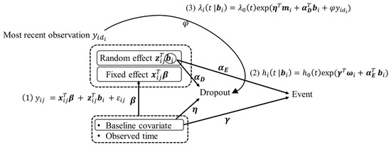
Figure 1.
Causal diagram for the proposed model that contains the three submodels.
2.2. Estimation
The unknown parameters included in the proposed model defined in Equations (1)–(3) are estimated by the Bayesian approach. The estimation procedure can be simplified under the assumption that random effects are normally distributed. The log-likelihood is given by:
where and are survival functions about event time and dropout time , respectively. is an indicator variable about dropout. is the full parameter. is the conditional probability density function for given and , and is the joint prior distribution for and . We developed a Bayesian inferential procedure based on the procedure proposed in [18]. A normal prior distribution was used for β, a Gamma distribution for , a normal distribution for the event part parameter vector and . For the variance–covariance matrix of the random effects D, we assumed inverse Wishart distribution. Prior independent gamma distributions were assumed for the baseline hazard parameters. Based on the likelihood and the prior distributions, the conditional posterior distributions were obtained. The detailed estimating procedure is referred to [18].
3. Numerical Results
In this section, our proposed model is evaluated through a simulation study and real data analysis by both using the dataset pbc2 included in R package JMbayes [19]. The pbc2 data are from the randomized placebo-controlled study of the drug D-penicillamine in primary biliary cirrhosis (PBC) of the liver conducted in the Mayo Clinic between 1974 and 1984. The data contains the longitudinal data of levels of serum bilirubin and time-to-death data with 312 patients. We used the data for the simulation study and real data analysis since much of the missing data was contained in the dataset.
3.1. Simulation
A simulation study was carried out to evaluate the performance of the proposed model relative to the performance of existing joint model using the JMbayes package and LMM using the nlme package [20] under the specific missing mechanism. Simulation data were produced by 300 subjects with a maximum follow-up time of 5 years, with 1000 replications. Longitudinal serum bilirubin levels were measured every 3 months. Using the R code provided by [18], we obtained the longitudinal data with the LMM as follows:
where fixed covariates from subject are represented by with parameter , and covariates for random effects are denoted with with random effect True values of each parameter are , and . For time-to-event data, we assumed the relative risk model as follows:
Under both scenarios, the longitudinal serum bilirubin level was missing after the event that depends on the random effect . In such a case, the missing mechanism is considered MNAR. Since the models for time-to-drop were different under these two scenarios, the simulation data under scenario 1 contains more parts conditioned on observed longitudinal value than the data under scenario 2 because of the difference of models for time-to-dropout.
The results of this simulation study are shown in Table 1. We observed that the association parameter estimates were less biased in our proposed model compared to the existing joint model in scenarios 1 and 2. About the slope estimate, it showed nearly the same bias in our proposed model compared to the LMM, whereas the empirical coverage probability showed better compared to the LMM and worse compared to the existing joint model. With each model, it was not indicated that there were differences between each estimate under these missing scenarios.

Table 1.
Performance of the different models under scenario 1 and scenario 2: results from 1000 replications with each dataset containing 300 subjects.
3.2. PBC2 Data Analysis
We applied the same models that we used in the above simulation study and evaluated the serum bilirubin’s trajectory and how it relates to relative risk of death. The results of this analysis are presented in Table 2. There was a difference between the slope estimate of LMM (2.50) and the slope estimate of the joint model (2.77), and the slope estimate of the proposed model was in the middle (2.65). The estimates of the association slope parameters were different between the joint model (0.48) and the proposed model (0.37). This difference might be caused by each assumption of missing mechanism. With the LMM, it is assumed that missing data are under MAR, whereas with the joint model it is assumed that missing data are under MNAR. The reasons for missing data might be the change in the longitudinal data and the risk of the event; therefore, it is indispensable to consider the latent variable’s influence on the missing data, and MNAR data contain MAR parts as noted [3]. Even if all missing reasons are known, it is still impossible to distinguish these missing mechanisms as MAR or MNAR. This is why there is a difference in the estimates between our proposed model and the existing model. Therefore, our model that does not need a strict assumption showed the middle value of the estimates in this gap. When the true missing mechanism is unknown, the models for which an extreme assumption of MAR or MNAR is needed might show some difference in their estimations. On the other hand, our proposed model, which does not need a strict assumption, might show an appropriate estimation.
Table 2.
Results from the pbc2 data with the proposed model, the existing JMbayes package, and the linear mixed model.
4. Discussion
In this paper, we proposed a novel joint model with which it is possible to assume a flexible assumption of missing data. We evaluated its performance through a simulation study. In this simulation study, we prepared two missing scenarios that are MNAR, but one scenario has the MAR counterpart more than the other scenario. Under both of these scenarios, our proposed model performed well in estimating the association parameters compared with the existing models. Under both scenarios, if we analyze them with a MAR assumption ignoring the latent variable, the results could lead to some biases, as shown in the slope estimates with the LMM. On the other hand, when we analyze them with MNAR assumption, not considering that the missing data depends on only observed values, the association parameter estimates were led to become seriously biased, as shown in the existing joint model result. These serious biases could be caused by strict MNAR assumption under the existing model. Otherwise, the slope estimates of the existing joint model were showed better than our proposed model. The reason why it is less biased in the association parameter estimates and more biased in slope estimates is that there might still be an undetectable missing mechanism in the data. Our simulation setting might still be a restrictive example, and it will be needed that a further simulation study should be performed in a more generated situation. With the results of the pbc2 data, it is shown that the extreme assumption can cause some biases. Under the assumptions of MAR and MNAR with the LMM and the joint model, there is a gap between these estimates, whereas the estimates of the proposed model showed a middle value of the gap. As it has already been pointed out, the missing data under MNAR might contain the counterpart fitting the observed data [3]. Therefore, even if our simulation study were performed under a restricted setting, we still support our conclusion that the analysis should be performed with no strict assumptions. In addition, our pbc2 results demonstrated the simulation study’s findings.
It is common to assume a strict missing mechanism in clinical study analysis. Even if we can assess the appropriateness of the assumption about the missing mechanism of obtained data, it might be impossible to distinguish the MAR counterpart in the MNAR data. Ideally, the statistical model should not be influenced by the strict proportion of missing mechanisms. When we desire to know the relation between the longitudinal data and some relative risk, the existing joint model is used as an analysis method or as a sensitive analysis method. We have showed the biased result of ignoring MAR under MNAR assumption. Our proposed model indicated that it could analyze data without a strict missing mechanism assumption of MAR or MNAR; we expect that our proposed model gives an appropriate and robust estimation that is not influenced by incorrect missing assumptions.
Author Contributions
Conceptualization, Y.T. and T.M.; methodology, Y.T. and T.M.; investigation, Y.T.; writing—original draft preparation, Y.T.; writing—review and editing, T.M. and K.Y.; visualization, Y.T.; supervision, T.M. and K.Y. All authors have read and agreed to the published version of the manuscript.
Funding
This research received no external funding.
Data Availability Statement
The data presented in this study are available in [19].
Conflicts of Interest
The authors declare no conflict of interest.
References
- Wulfsohn, M.S.; Tsiatis, A.A. A joint model for survival and longitudinal data measured with error. Biometrics 1997, 53, 330–339. [Google Scholar] [CrossRef]
- Tsiatis, A.; Davidian, M. An overview of joint modeling of longitudinal and time-to-event data. Stat. Sin. 2004, 14, 793–818. [Google Scholar]
- Molenberghs, G.; Beunckens, C.; Sotto, C.; Kenward, M.G. Every missingness not at random model has a missingness at random counterpart with equal fit. J. R. Stat. Soc. Ser. B Stat. Methodol. 2008, 70, 371–388. [Google Scholar] [CrossRef]
- Rubin, D.B. Inference and missing data. Biometrika 1976, 63, 581–592. [Google Scholar] [CrossRef]
- Little, R.J.A.; Rubin, D.B. Statistical Analysis with Missing Data, 2nd ed.; John Wiley and Sons: New York, NY, USA, 2002. [Google Scholar]
- Little, R.J. Pattern-mixture models for multivariate incomplete data. J. Am. Stat. Assoc. 1993, 88, 125–134. [Google Scholar]
- Little, R.J. A class of pattern-mixture models for normal incomplete data. Biometrika 1994, 81, 471–483. [Google Scholar] [CrossRef]
- Little, R.J. Modeling the drop-out mechanism in repeated-measures studies. J. Am. Stat. Assoc. 1995, 90, 1112–1121. [Google Scholar] [CrossRef]
- Wu, M.C.; Carroll, R.J. Estimation and comparison of changes in the presence of informative right censoring by modeling the censoring process. Biometrics 1988, 44, 175–188. [Google Scholar] [CrossRef]
- Wu, M.C.; Bailey, K.R. Estimation and comparison of changes in the presence of informative right censoring: Conditional linear model. Biometrics 1989, 45, 939–955. [Google Scholar] [CrossRef]
- Follmann, D.; Wu, M. An approximate generalized linear model with random effects for informative missing data. Biometrics 1995, 51, 151–168. [Google Scholar] [CrossRef] [PubMed]
- Molenberghs, G.; Vereke, G. Models for Discrete Longitudinal Data; Springer: New York, NY, USA, 2005. [Google Scholar]
- Molenberghs, G.; Kenward, M.G. Missing Data in Clinical Studies; Wiley: Chichester, UK, 2007. [Google Scholar]
- Creemers, A.; Hens, N.; Aerts, M.; Molenberghs, G.; Verbeke, G.; Kenward, M.G. A sensitivity analysis for shared-parameter models for incomplete longitudinal outcomes. Biom. J. 2010, 52, 111–125. [Google Scholar] [CrossRef]
- Creemers, A.; Hens, N.; Aerts, M.; Molenberghs, G.; Verbeke, G.; Kenward, M.G. Generalized shared-parameter models and missingness at random. Stat. Model. 2011, 11, 279–310. [Google Scholar] [CrossRef]
- Njagi, E.N.; Molenberghs, G.; Kenward, M.G.; Verbeke, G.; Rizopoulos, D. A characterization of missingness at random in a generalized shared-parameter joint modeling framework for longitudinal and time-to-event data, and sensitivity analysis. Biom. J. 2014, 56, 1001–1015. [Google Scholar] [CrossRef] [PubMed]
- Papageorgiou, G.; Rizopoulos, D. An alternative characterization of MAR in shared parameter models for incomplete longitudinal data and its utilization for sensitivity analysis. Stat. Model. 2021, 21, 95–114. [Google Scholar] [CrossRef]
- Thomadakis, C.; Meligkotsidou, L.; Pantazis, N.; Touloumi, G. Longitudinal and time-to-drop-out joint models can lead to seriously biased estimates when the drop-out mechanism is at random. Biometrics 2019, 75, 58–68. [Google Scholar] [CrossRef] [PubMed]
- Rizopoulos, D. The R Package JMbayes for Fitting Joint Models for Longitudinal and Time-to-Event Data Using MCMC. J. Stat. Softw. 2016, 72, 1–46. [Google Scholar] [CrossRef]
- Pinheiro, J.C.; Bates, D.M. Mixed-Effects Models in S and S-PLUS; Springer: New York, NY, USA, 2000. [Google Scholar]
Publisher’s Note: MDPI stays neutral with regard to jurisdictional claims in published maps and institutional affiliations. |
© 2022 by the authors. Licensee MDPI, Basel, Switzerland. This article is an open access article distributed under the terms and conditions of the Creative Commons Attribution (CC BY) license (https://creativecommons.org/licenses/by/4.0/).