1. Introduction
The rapid development of information technology not only brings great convenience to network users but also brings many security threats. Network traffic is an important carrier for network information exchange and transmission. Many network attacks and threats also exist in network traffic, so malicious traffic classification is one of the research focuses of cyberspace security. Due to the wide application of application-layer encryption technology, traditional port matching [
1], deep packet inspection (DPI) [
2,
3,
4], and other technologies cannot accurately identify malicious traffic. Therefore, researchers try to classify malicious traffic using various machine learning algorithms such as SVM, decision tree, naive Bayes, etc. However, machine learning-based methods involve two problems. First, machine learning models always rely on the knowledge and experience of professional security personnel to extract and select traffic features. Second, machine learning models have low accuracy and poor generalization ability in multi-classification tasks. Compared with machine learning, deep learning is a more popular method. As an end-to-end learning method, it can automatically extract data features without human intervention. Although the deep learning network enhances the expressive power, the performance of this classification algorithm decreases in the case of an imbalanced class distribution of the dataset, especially for few samples.
Therefore, overcoming imbalanced class distribution is of great significance for the classification of malicious traffic. To solve the problem of poor generalization of the classification model and the feature representation in the case of a class imbalance dataset, a representation method based on the Markov transition matrix and Adversarial Generative Networks with Filters (Filter-GAN) is proposed in this paper.
The original input to the feature representation method is the traffic session. The method embeds the relevant features into the feature image through the feature image extraction algorithm. The feature images are then used to train a Generative Adversarial Network (GAN) model and data filter based on machine learning algorithms. Finally, the GAN model generates enough new samples to filter out more effective samples through the data filter. These more effective samples serve as a supplement to the original dataset to address the problem of sample imbalance.
Compared with traditional malicious traffic characterization methods and data enhancement methods, this method has a better feature representation effect and stronger data enhancement effect, which can make the classification model have a better generalization and higher classification accuracy. There are two main contributions of this paper:
A new traffic feature representation method is proposed. The method embeds the header feature and payload feature of each data packet into a feature image, which realizes a unified representation method for traffic files. The method avoids information loss and redundancy during preprocessing because the traffic session file is not sliced or populated. Compared with the traditional grayscale image method, the feature image generated by this method is more friendly to the model.
A generative adversarial network model with a sample filter is designed. The filter is trained and tested with real samples to screen the generated samples so that the generated samples that pass the screening are closer to the distribution of real samples.
The rest of the paper is organized as follows. The second part introduces the related work of malicious traffic classification. The third part elaborates the whole model framework and training process, including data preprocessing, feature image extraction, model structure, and algorithm.
Section 4 describes the experimental details and result evaluation.
Section 5 concludes and proposes future work.
2. Related Work
2.1. Classification of Malicious Traffic Based on Deep Learning
Deep learning has been widely used [
5,
6,
7,
8,
9,
10] in the field of traffic detection and classification. Wang et al. [
11] combined deep learning with traffic analysis for the first time, pointing out the similarities between images and TCP traffic. Jia et al. [
12] further studied the application of deep learning in traffic analysis, unifying the length of the data packets, so that the length of each data packet reaches 784 bytes. The flow vector is converted into a 28 × 28 byte matrix and fed into a convolutional neural network for malicious traffic classification. Wang et al. [
13] converts the data packets of the same five-tuple into fixed-length byte vectors in sequence according to time and then forms feature vectors through data compression. The feature vector is classified using the convolutional neural network with the Gabor function to achieve the purpose of intrusion detection. The two methods inevitably fill or intercept bytes, resulting in loss of information.
Jiarui Man et al. [
14] directly used 196 statistical features of malicious traffic to form images, and then used a residual network for intrusion detection. Although the use of a residual network has good advantages in multi-classification, this method does not consider that there is no spatial position information between statistical features. Simply converting a one-dimensional vector into a two-dimensional matrix causes redundancy of information. Huiwen Bai et al. [
15] convert network traffic into text, in which the words in the text consist of every byte of the payload. We use the n-gram semantic neural network model to generate continuous domain vectors, and then use the gated recurrent unit (GRU) to obtain feature vectors for final classification. However, with the use of more encryption protocols, the packet payload is randomly encrypted and no longer has specific semantics. This makes semantic-based malicious traffic detection difficult. Marín [
16] takes the network traffic byte stream directly as the input of the convolutional neural network and the recurrent neural network, and evaluates the feature representation effect at the packet and flow level. There are also many related works [
17,
18,
19,
20] that demonstrate the superiority of deep learning (DL) methods for malicious traffic analysis. We conclude that the DL method application technique consists of three steps: First, converting the data packet or pcap file into the standard input format of DL, then selecting a deep learning model according to the characteristics of the input data, and finally training the DL classifier to automatically extract and classify the characteristics of the traffic.
2.2. Common Methods for Dealing with Sample Imbalances
In the field of network traffic classification, the class imbalance problem can be expressed as an order of magnitude difference in the number of samples of traffic data in each application category, resulting in the classifier being overwhelmed by the majority class and ignoring the minority class. Misidentifying small categories is often costly. For example, in intrusion detection, the attack class is a small class relative to normal traffic, and misclassifying the attack class may cause network paralysis. There are generally three ways to deal with data imbalance: modify the objective cost function, change the sampling strategy, and generate artificial data as shown in
Table 1. The method of modifying the loss function can alleviate the problem of quantity imbalance through different weighting processes according to different sample sizes. This approach gives higher scores to small classes and penalizes large classes for updating the parameters of the classification model.
Methods to address sample imbalance also include random undersampling (RUS) and random oversampling (ROS) strategies [
21,
22,
23]. Undersampling increases the number of samples in the secondary class by discarding some sample data, thereby reducing the sample size in the main class. Oversampling increases the amount of data for samples with fewer classes by reusing data from classes with fewer classes. However, if the sample size of the minority class is very small, then discarding a large number of samples from the majority class will result in a loss of sample distribution information. While the oversampling method repeats samples leading to severe overfitting problems, which has been the main disadvantage of oversampling.
As a method of oversampling, SMOTE (Adaptive Synthetic Sampling) [
24] is also widely used in the literature to solve the class imbalance problem. However, it relies on interpolation for oversampling, resulting in poor representation of synthetic samples. SVM-SMOTE method [
26] use support vector machine (SVM) classifiers to train the support vectors on the original training set. Based on the majority sample density of the nearest neighbors, interpolation or extrapolation techniques are used to combine each minority class support vector with its nearest neighbors to generate new samples. Chen et al. [
25] proposed the ADASYN (Adaptive Synthetic Sampling) method for data generation based on the SMOTE method. However, the experimental results show that the distribution of the generated data is quite different from the real data. Last et al. [
27] applied the Kmeans algorithm to the SMOTE method, taking inter- and intra-class relationships into account in the generated data.
The classic approach to generating artificial data is based on Generative Adversarial Networks (GAN), which are trained using a few samples as training data, rather than simply replicating it. Related research [
28] shows that GANs can efficiently generate high-quality synthetic samples. Vu et al. [
29] used the GAN model to generate data to supplement a small number of categories. The SVM, decision tree, and random forest models were trained on mixed data and achieved high classification accuracy. Wang et al. [
30] generated multiple minority class data simultaneously through a conditional GAN model. The generated data are then supplemented by the minority class, which effectively improved the accuracy compared to the original dataset. Wang et al. [
31] used a GAN model for data generation on an unbalanced encrypted traffic dataset in units of network flows. Although perceptrons have been widely used to solve class imbalance problems, instability problems such as vanishing gradients, mode collapse, etc. have always been shortcomings of multilayer perceptrons. Furthermore, they do not evaluate the data distribution of the generated samples versus the real samples. Therefore, in this paper, we propose to use filters trained on real samples to filter the generated samples, directly avoiding crashes and instability problems in the model. At the same time, the generated samples are evaluated using mathematical statistical methods.
3. The Proposed Method
This section discusses the framework for malicious traffic classification based on the Filter-GAN model, shown in
Figure 1. It is divided into three stages: the data processing stage, data enhancement stage, and classification stage. In particular, the difference between the Filter-GAN model-based framework and the general method framework is the data processing stage and the data augmentation stage.
In the data processing stage, the original traffic file is divided into network session files according to the network quintuple. The network session file is used as the input of the feature image algorithm. The algorithm generates data matrices of uniform size without filling or intercepting valid fields. Then, these data matrices are converted into feature images to form feature image datasets.
The data augmentation stage is mainly used to generate data to supplement the minority class. Due to the imbalanced distribution of categories in the original traffic dataset, the feature image set still suffers from imbalanced problem. Therefore, firstly, through the adversarial generative network (GAN), enough new feature images are generated and sent to the filter to screen more effective samples as a supplement to the original feature image set to enhance the diversity of the original feature images. It is worth mentioning that here, the generator generates feature images instead of the original raw traffic files.
In the classification stage, a convolutional neural network model is used as the classification model. The training set and the test set are the mixed feature image dataset and the original feature image dataset, respectively. Finally, the classification effect is evaluated.
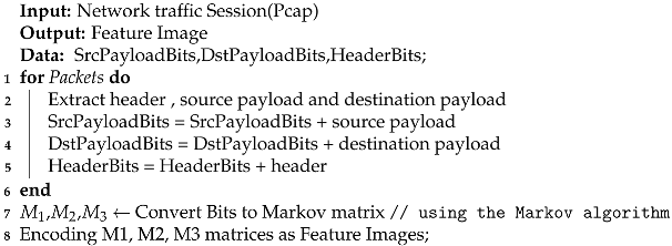
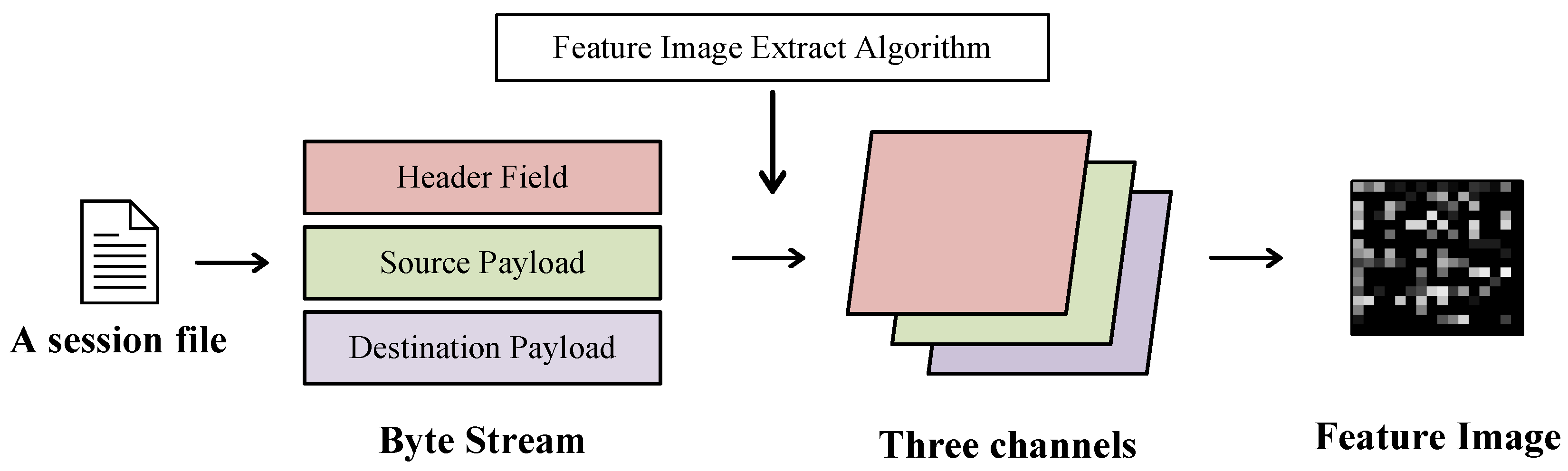
3.1. Feature Image Extraction Algorithm
Traffic sessions have statistical, timing, and payload-related features. To compress all the features into one image as much as possible and improve the representation ability of the feature image, the feature image extraction algorithm converts the header field, source payload, and destination payload into three matrices, which are compressed into three channels of a picture to form a complete feature image. The specific process is shown in
Figure 2.
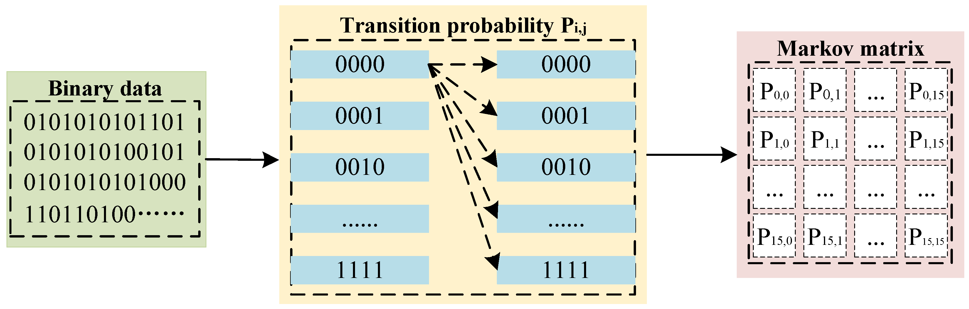
There are data packets in two directions in a network session and the header fields of the information about the data packets themselves. The header field of each data packet needs to remove noise and useless information, such as data link layer information (mac address, frame type, etc.), and truncates the IP address. These data can usually be regarded as a bit stream, and each bit string has different state transition probabilities. This transmission process has the characteristics of a Markov chain. Therefore, the use of Markov models can effectively characterize the spatiotemporal features of session payloads.
We read the header field and payload of each data packet in the session file in binary mode, and then divide the payload into source payload and destination payload. Then, we take every four bits as a value. It can be expressed as:
where
N is the byte length and the vector
v is the encoded state vector. Consider
v as a Markov chain, calculate the probability that two adjacent states
appear after
, denoted by
:
where
. All can form a Markov probability transition matrix:
Figure 3 is the process of converting binary data into a Markov matrix. Each value of the Markov matrix of malicious traffic is the transmission probability of a fixed-length bit string, not the actual value of the bit string. They represent the distribution characteristics of network session fields. After converting the payload and the header fields into Markov matrices, they are used as three channels of the feature image, respectively. Each value in the matrix is used as a pixel point of the feature image to form a feature image as in feature image extraction Algorithm 1.
| Algorithm 1: Feature Image Extract |
![Mathematics 10 03482 i001]() |
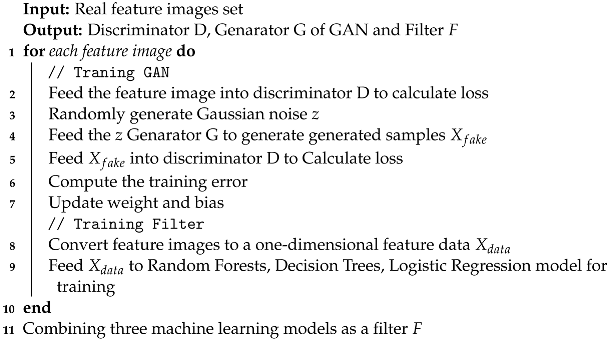
3.2. Filter-Gan Model Based on Gan with Machine Learning Filter
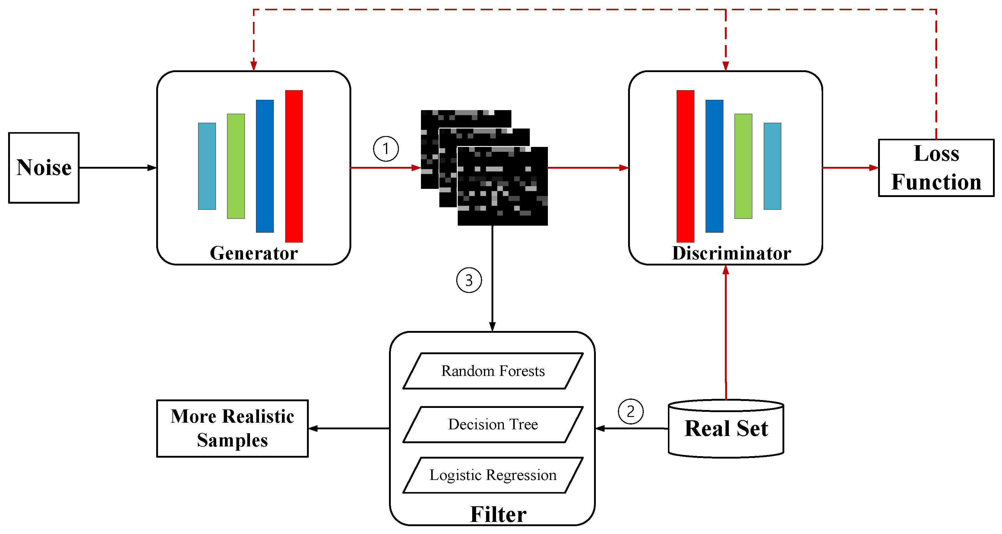
The structure of Filter-GAN is shown in
Figure 4, including generator, discriminator, and sample filter. The first step is GAN network training. Random noise is sent to the generator to generate enough samples, then the generated samples and real samples are sent to the discriminator for backward propagation of the loss function so that the entire model can generate a generated sample that is closer to the real sample image. In the second step, the filter consisting of a machine learning model uses real data for training and testing. When the best classification effect is achieved, it is used to screen the samples generated in the first step. In step 3, the samples generated by the GAN model are fed into the filter to screen more effective samples.
3.2.1. Gan Model and Loss Function
GAN [
32] includes a generator (
G) and a discriminator (
D). The structure of the GAN network model constructed in this paper is shown in
Table 2 and
Table 3. In the original imbalanced data, for the minority attack class, the real sample
is randomly selected as the input of
D.
is the output of
D, representing the probability that the data distribution of
belongs to the real data distribution
. A noise vector
is randomly generated in the normal distribution
as the input to
G.
G generates synthetic samples
. This generated sample is then used as the input of the discriminator, which is used to predict the probability
of
in the generated data distribution
.
The objective function of GAN is given as follows:
The purpose of GAN is to maximize the discriminator D and minimize the generator G. and are the probability distributions of the real data and latent vectors, respectively.
Accordingly, the loss functions of
D and
G are:
3.2.2. Sample Filter Based on Machine Learning
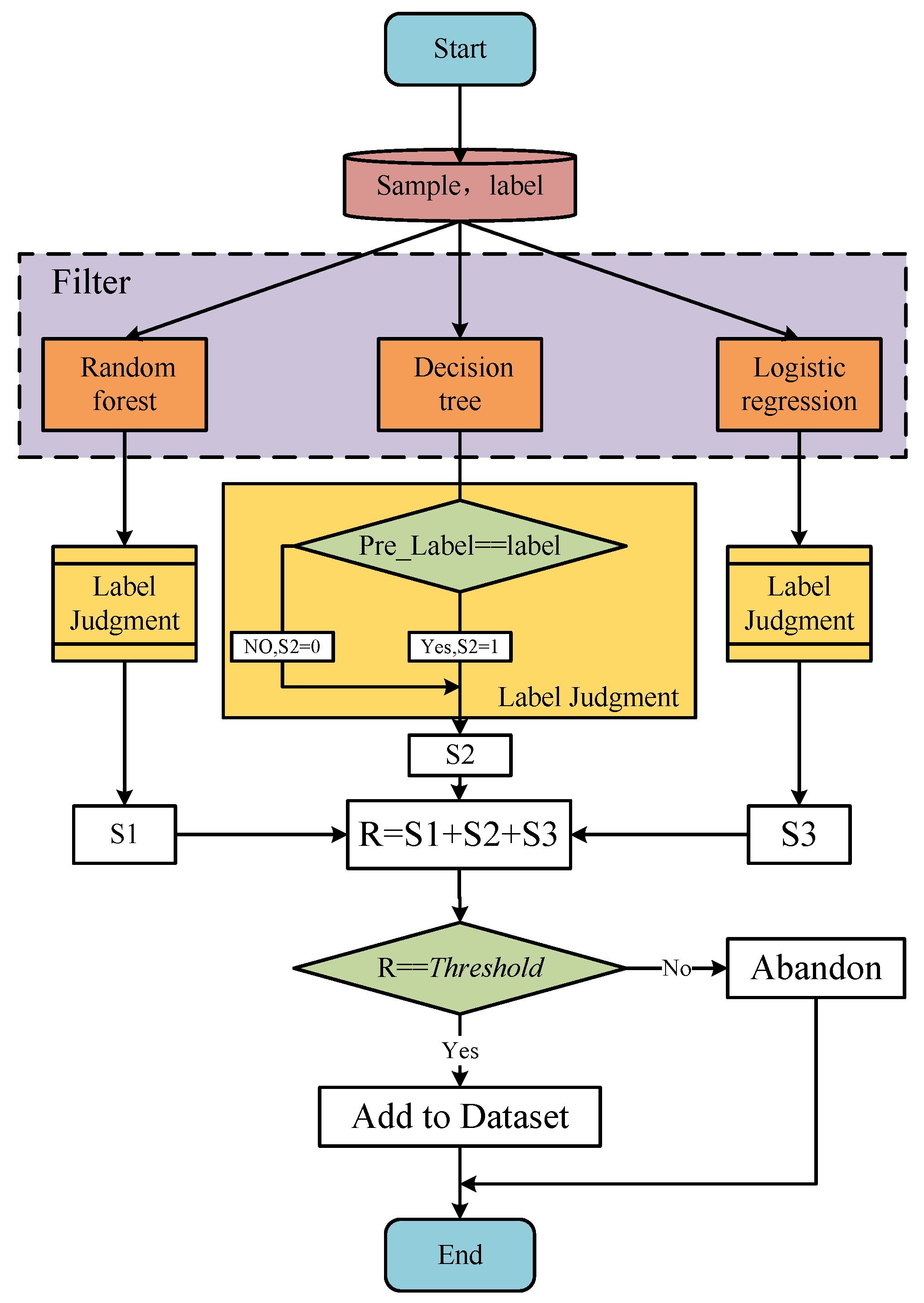
GAN uses the maximum similarity to measure the loss of the entire model training. When the data are distributed in high dimensions, the similarity of the data is difficult to define, which can cause the generated samples to not be close to the real samples. However, since GAN models can generate infinite samples, we use decision trees, random forests, and logistic regression models to compose a sample filter to filter the generated samples. The screening process is shown in
Figure 5.
Each generated sample with a label is sent to three machine learning models to obtain predicted labels. The value is 1 if the predicted label is the same as the label of the generated sample, and 0 otherwise. Finally, we add the results of the three models to obtain R, . For example, when a sample obtains through the filter, meaning that the sample is judged to be of this class by the two machine learning models in the filter.
To limit the filtering granularity of the filter, a
is set. If
R is greater than or equal to the
, the generated sample is added to the dataset, otherwise, it is discarded. Algorithm 2 is the training process of Filter-GAN.
| Algorithm 2: Filter-GAN Training process. |
![Mathematics 10 03482 i002]() |
4. Experimental Evaluation
4.1. The Datasets and Evaluation Metrics
4.1.1. Malicious Traffic Dataset
The dataset in the experiments comes from the Malware Capture Facility project [
33], which collects malicious traffic over a long period. The datasets released by this project contain malicious traffic generated by various malicious attack methods, such as ransomware, DDoS attacks, and Trojan horse attacks. Many of these malicious programs cannot generate enough network traffic during the attack or propagation process, resulting in an imbalanced number of malicious traffic samples.
Twelve types of malicious traffic were selected. The SplitCap.exe tool [
34] was used to split the original traffic file PCAP into network sessions, which were converted to feature images using the feature image extraction algorithm.
In
Table 4, it can be seen that there is an extreme imbalance between the samples. For example, MinerTrojan’s samples only accounted for 1.23% of the entire dataset, and PUA only accounted for 0.69% of the entire dataset. Therefore, there was a distribution imbalance problem between the categories of this dataset, which can be used to verify the method and model proposed in this paper.
4.1.2. Evaluation Metrics
To evaluate the performance of our method on imbalanced datasets from multiple perspectives, we used accuracy, precision, recall, and
F1:
4.1.3. Experimental Platform and Configuration
The training and testing of the model have been carried out under the Windows 10 operating system. The deep learning model was implemented using the Python language based on the Torch framework. The parameters are listed in
Table 5.
4.2. Experimental Results and Analysis
The experiment was carried out from two aspects, the first is to prove whether the feature extraction algorithm can effectively characterize malicious traffic. The second is to prove the data generation model and data filter proposed in this paper, which can effectively supplement the samples with an unbalanced number of samples.
4.2.1. Feature Image Representation Ability Experiment
To verify that the feature extraction algorithm proposed in this paper can effectively characterize malicious network traffic, the feature image sets obtained after data processing are respectively sent to the machine learning model and the neural network model for multi-classification experiments. Machine learning models include random forest (rf), decision trees (dt), and logistic regression (lr) models.
In the machine learning model, each pixel of the three-dimensional feature image (dimension (3, 16, 16)) is regarded as a feature, converted into a one-dimensional vector with a feature number of 768, and normalized as a machine input to the learning model. The neural network model includes the residual convolutional neural network (res, ResNet), which directly uses the three-dimensional feature image as the input of the model. The training parameters are shown in
Table 6.
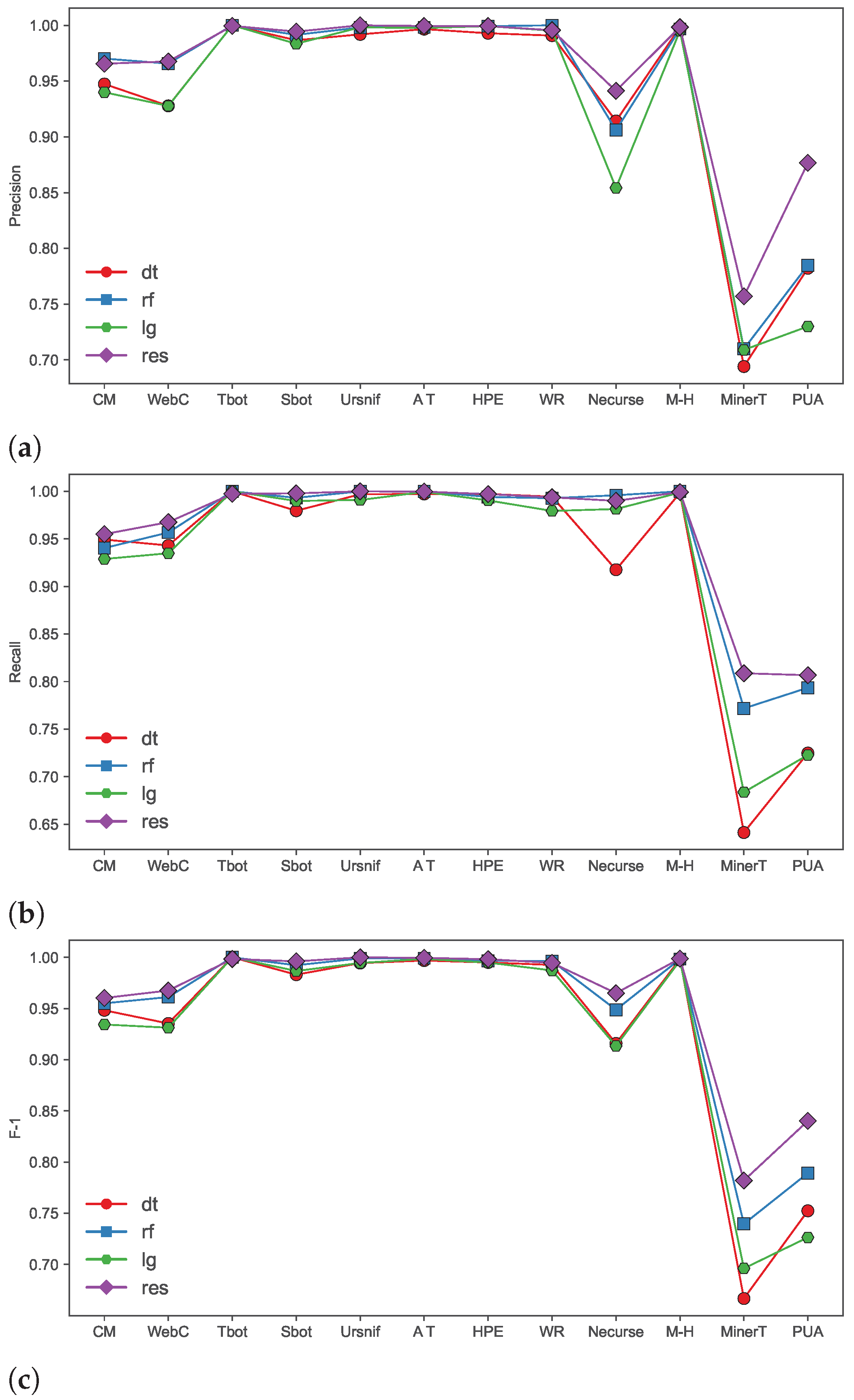
The results of Precision, Recall, and F1 for each category in the classification results are shown in
Figure 6. the classification effects of various categories are the ResNet model, Random Forest, Decision Tree, and Logistic Regression. The ResNet model performs significantly better than the machine learning model, because the feature images generated by the feature image extraction algorithm are essentially three-channel images. Each pixel on the image is the transition probability of a fixed-length bit string in the traffic field, which represents the feature distribution of the field. In the field of image classification, ResNet has a very large advantage, so the results of the ResNet model are better than the classification results of the machine learning model. At the same time, it also shows that the feature image extraction algorithm proposed can effectively extract malicious traffic session features when there are enough samples in the dataset.
In an addition,
Figure 6 shows the detection accuracy of each category using the ResNet model, which shows results above 0.95 for most classes, except Necurse, MinerTrojan, and PUA. In particular, the number of samples in these three categories accounts for less than 2% of the total number of samples, and the number of training samples is less than 1000, which is very small as the amount of pre-training data for deep learning models. Therefore, the reason for the low classification accuracy of these three categories is largely due to the insufficient number of samples, resulting in the imbalance of sample classes.
To solve this problem, in the following experiments, according to the distribution of the sample size of the original dataset, Filter-GAN was used to perform data enhancement for the categories with less than 10,000 samples.
4.2.2. Data Generation and Dataset Balancing
The network session was transformed into feature images through feature extraction algorithms to form feature image datasets. The number of various feature images in the feature image set also inherits this shortcoming due to the unbalanced number of web sessions per class. According to the results of the above experiments, it can be seen that the imbalance in the amount of data between samples leads to poor classification results.
Therefore, for categories with less than 10,000 feature images in the dataset, including WebCompanion, Necurse, MinerTrojan, and PUA, the Filter-GAN model was used for data augmentation. These feature image datasets were trained as input to the GAN model in Filter-GAN. The featured image was then converted into a 1D vector (one feature per pixel) and fed to the filter for training. Finally, the trained GAN model was used for sample generation, and the generated samples were screened by the filter. The samples generated by screening were closer to the data distribution of the real samples.
Samples that can pass the filter were selected and those that did not pass were discarded directly. Because a GAN model can use random noise as input, it can keep generating samples until enough valid samples are generated.
Figure 7 shows the comparison of the amount of data before and after the four small sample balances in the dataset so that the entire dataset achieves class balance.
To highlight the effect of the filter, we use the following statistical methods to compare the effectiveness of generated samples and real data. Considering the real data samples , and the generated data samples , where . The average of the real and generated data samples is computed as and , respectively.
Euclidean distance: Euclidean distance (
) is used to evaluate the distance of two samples in Euclidean space. As shown in Equation (
12), the lower ED indicates that the real sample and the generated sample are more similar.
Correlation Coefficient: The Pearson correlation coefficient (
) assesses the correlation between two samples, as shown in Equation (
13). The higher the correlation between the two samples, the closer the
is to 1.
Fréchet distance: The Fréchet distance (
) is given by Equation (
14). Evaluating the distance of two samples in metric space is a robust measure relative to Euclidean distance. A lower FD indicates that the two samples are more similar.
In order to evaluate the effect of the filter, we set different
, including 1, 2, and 3, to generate sample screening. For example, a threshold of 2 indicates that the generated samples pass both machine learning models in the filter. The generated samples of each class are screened, and the similarity estimates are calculated with the real samples, including ED, CC, and FD. The results are shown in
Table 7.
For the result of each class of samples and each threhold, the result that generated samples pass the three machine learning models in the filter is the best; that is, the ED and FD are the smallest, and the CC value is the largest. This shows that the filter built by machine learning is able to filter out generated samples that are more similar to the real samples. In other words, compared with the general GAN model, the samples that Filter-GAN generate are closer to the real samples.
4.2.3. Experimental Results on Balanced Datasets
To compare the filtering effect of Filter on the generated samples. Experiments are carried out on imbalanced datasets and balanced datasets with different filter thresholds. As can be seen in
Section 3.2.2, when the threshold = 1 is set, the sample passes only one machine learning model in the filter. As can be seen from
Table 8, when only the imbalance feature image set is used as the training set for classification, the accuracy of the small sample categories such as Necurse, MinerTrojan, and PUA is very low.
When using a balanced dataset with the filter, . We use generated feature image samples as a complement to the few-shot class training set. Compared with using only the imbalanced dataset, the classification accuracy of this case is not significantly improved, which is large because the data distribution of the samples generated by the GAN network is not close to the real samples. That is to say, the sample size of these four types of samples used to train the GAN network model is too small so that the GAN network model cannot fully learn the data distribution of the small sample category so that the generated samples of effective data distribution cannot be accurately generated. Therefore, it is necessary to use filters to screen the generated samples.
When the or 3, the generated samples as supplementary four-type small samples pass the classification of at least one machine learning model in the filter. The results show that the classification results of MinerTrojan, WebCompanion, and Necurse are improved. The F-1 indicators all rose above 0.97. Necurse’s Precision and F-1 metrics improved by 1%. In particular, the MinerTrojan category achieved an accuracy of 0.8187, an improvement of 6%. This shows that through the filtering of the filter, the data distribution of the generated samples is closer to the real samples, which effectively solves the problem of class imbalance in the real dataset. Filter-GAN considers the diversity and accuracy of the generated samples, making the classification effect of the samples more significant.
4.2.4. Comparative Experiment
We implement the commonly used methods for dealing with data imbalance as a comparative experiment for Filter-GAN. The first method is
the Random Oversampling (ROS) [
22], which aims to improve the sampling rate of small classes. ROS generates some copies of the secondary class examples. The method is simple to implement and requires little computation. The second way is the
synthetic minority over-sampling technique (SMOTE) [
24]. The SMOTE method generates samples by evaluating the feature space of the sample and its k-nearest neighbors, where
k is determined by the number of minority samples. Specifically, first let the
vector be different from the feature vector of the minority sample
, that is, the
k nearest neighbors, let
where
. Then, the new sample
. Further, some derivatives of SMOTE are also implemented, such as SVM-SMOTE [
26], ADASYN [
25].
Table 9 shows the results of the comparison experiments. The table shows the overall accuracy for the classification task and the classification accuracy for the four minority classes. The overall accuracy of our method is higher than other methods. Secondly, the accuracy rates of CM, WebC, MinerT, and PUA are also higher than other research methods. Therefore, the Filter-GAN method outperforms other compared methods, which shows that our method has advantages in malicious traffic characterization and data augmentation.
5. Conclusions
The class imbalance of malicious traffic datasets leads to the low classification accuracy of deep learning and weak generalization ability. It is solved by two aspects in this paper: on the one hand, the features of the network session are mapped to the feature image, which makes the low-rank feature space of the image represent the diversity of the original traffic session. This method can generate images of uniform size and realize the uniform expression of features in different sessions. On the other hand, to balance the original traffic session dataset, the Filter-GAN model continuously generates new feature images through the GAN model and uses filter to filter the generated samples, so that the generated samples are closer to the distribution of real data. Experimental results show that the feature image representation method can effectively classify malicious traffic families. When there are enough class samples, the detection accuracy of the samples can reach 99%. In the case of unbalanced samples of malicious traffic families, after using the Filter-GAN model to enhance the small sample data, the detection and classification accuracy is also significantly improved up to 6%.
Author Contributions
Conceptualization, X.C. and Q.L.; methodology, X.C.; software, P.W.; resources, X.C.; data curation, X.C.; writing—original draft preparation, X.C.; writing—review and editing, X.C.; visualization, P.W.; supervision, Q.L.; project administration, P.W.; funding acquisition, Q.L. All authors have read and agreed to the published version of the manuscript.
Funding
This research was funded by the National Natural Science Foundation of China under Grant 61902328 and Key R&D projects of Sichuan Science and technology plan (2022YFG0323).
Data Availability Statement
The data presented in this study are available on request from the corresponding author. The data are not publicly available due to lab privacy.
Acknowledgments
The authors wish to thank the editor and the anonymous reviewers for their valuable suggestions on improving this paper.
Conflicts of Interest
The authors declare no conflict of interest.
References
- Cotton, M.; Eggert, L.; Touch, D.J.D.; Westerlund, M.; Cheshire, S. Internet Assigned Numbers Authority (IANA) Procedures for the Management of the Service Name and Transport Protocol Port Number Registry. RFC 6335. 2011. Available online: https://www.rfc-editor.org/info/rfc6335 (accessed on 24 October 2020).
- Khalife, J.; Hajjar, A.; Diaz-Verdejo, J. A multilevel taxonomy and requirements for an optimal traffic-classification model. Int. J. Netw. Manag. 2014, 24, 101–120. [Google Scholar] [CrossRef]
- Park, B.C.; Won, Y.J.; Kim, M.S.; Hong, J.W. Towards automated application signature generation for traffic identification. In Proceedings of the NOMS 2008—2008 IEEE Network Operations and Management Symposium, Bahia, Brazil, 7–11 April 2008; pp. 160–167. [Google Scholar]
- Sherry, J.; Lan, C.; Popa, R.A.; Ratnasamy, S. Blindbox: Deep packet inspection over encrypted traffic. In Proceedings of the 2015 ACM Conference on Special Interest Group on Data Communication, London, UK, 17–21 August 2015; pp. 213–226. [Google Scholar]
- Zhang, K.; Wang, Z.; Chen, G.; Zhang, L.; Yang, Y.; Yao, C.; Wang, J.; Yao, J. Training effective deep reinforcement learning agents for real-time life-cycle production optimization. J. Pet. Sci. Eng. 2022, 208, 109766. [Google Scholar] [CrossRef]
- Yin, F.; Xue, X.; Zhang, C.; Zhang, K.; Han, J.; Liu, B.; Wang, J.; Yao, J. Multifidelity genetic transfer: An efficient framework for production optimization. SPE J. 2021, 26, 1614–1635. [Google Scholar] [CrossRef]
- Zhang, K.; Zhang, J.; Ma, X.; Yao, C.; Zhang, L.; Yang, Y.; Wang, J.; Yao, J.; Zhao, H. History matching of naturally fractured reservoirs using a deep sparse autoencoder. SPE J. 2021, 26, 1700–1721. [Google Scholar] [CrossRef]
- Ma, X.; Zhang, K.; Zhang, L.; Yao, C.; Yao, J.; Wang, H.; Jian, W.; Yan, Y. Data-driven niching differential evolution with adaptive parameters control for history matching and uncertainty quantification. SPE J. 2021, 26, 993–1010. [Google Scholar] [CrossRef]
- Xu, X.; Wang, C.; Zhou, P. GVRP considered oil-gas recovery in refined oil distribution: From an environmental perspective. Int. J. Prod. Econ. 2021, 235, 108078. [Google Scholar] [CrossRef]
- Xu, X.; Hao, J.; Zheng, Y. Multi-objective artificial bee colony algorithm for multi-stage resource leveling problem in sharing logistics network. Comput. Ind. Eng. 2020, 142, 106338. [Google Scholar] [CrossRef]
- Wang, Z. The applications of deep learning on traffic identification. BlackHat USA 2015, 24, 1–10. [Google Scholar]
- Jia, W.; Liu, Y.; Liu, Y.; Wang, J. Detection Mechanism Against DDoS Attacks based on Convolutional Neural Network in SINET. In Proceedings of the 2020 IEEE 4th Information Technology, Networking, Electronic and Automation Control Conference (ITNEC), Chongqing, China, 12–14 June 2020; Volume 1, pp. 1144–1148. [Google Scholar]
- Wang, Y.; Jiang, Y.; Lan, J. Fcnn: An efficient intrusion detection method based on raw network traffic. Secur. Commun. Netw. 2021, 2021, 5533269. [Google Scholar] [CrossRef]
- Man, J.; Sun, G. A residual learning-based network intrusion detection system. Secur. Commun. Netw. 2021, 2021, 5593435. [Google Scholar] [CrossRef]
- Bai, H.; Liu, G.; Liu, W.; Quan, Y.; Huang, S. N-gram, semantic-based neural network for mobile malware network traffic detection. Secur. Commun. Netw. 2021, 2021, 5599556. [Google Scholar] [CrossRef]
- Marín, G.; Caasas, P.; Capdehourat, G. Deepmal-deep learning models for malware traffic detection and classification. In Data Science–Analytics and Applications; Springer: Berlin/Heidelberg, Germany, 2021; pp. 105–112. [Google Scholar]
- Hwang, R.H.; Peng, M.C.; Huang, C.W.; Lin, P.C.; Nguyen, V.L. An unsupervised deep learning model for early network traffic anomaly detection. IEEE Access 2020, 8, 30387–30399. [Google Scholar] [CrossRef]
- Wang, W.; Zhu, M.; Wang, J.; Zeng, X.; Yang, Z. End-to-end encrypted traffic classification with one-dimensional convolution neural networks. In Proceedings of the 2017 IEEE International Conference on Intelligence and Security Informatics (ISI), Beijing, China, 22–24 July 2017; pp. 43–48. [Google Scholar]
- Zhang, W.; Wang, J.; Chen, S.; Qi, H.; Li, K. A framework for resource-aware online traffic classification using cnn. In Proceedings of the 14th International Conference on Future Internet Technologies, Phuket, Thailand, 7–9 August 2019; pp. 1–6. [Google Scholar]
- Lotfollahi, M.; Jafari Siavoshani, M.; Shirali Hossein Zade, R.; Saberian, M. Deep packet: A novel approach for encrypted traffic classification using deep learning. Soft Comput. 2020, 24, 1999–2012. [Google Scholar] [CrossRef]
- Wang, P.; Chen, X. SAE-based encrypted traffic identification method. Comput. Eng. 2018, 44, 140–147. [Google Scholar]
- Vu, L.; Van Tra, D.; Nguyen, Q.U. Learning from imbalanced data for encrypted traffic identification problem. In Proceedings of the Seventh Symposium on Information and Communication Technology, Ho Chi Minh, Vietnam, 8–9 December 2016; pp. 147–152. [Google Scholar]
- Cieslak, D.A.; Chawla, N.V.; Striegel, A. Combating imbalance in network intrusion datasets. In Proceedings of the GrC. Citeseer, Atlanta, GA, USA, 10–12 May 2006; pp. 732–737. [Google Scholar]
- Chawla, N.V.; Bowyer, K.W.; Hall, L.O.; Kegelmeyer, W.P. SMOTE: Synthetic minority over-sampling technique. J. Artif. Intell. Res. 2002, 16, 321–357. [Google Scholar] [CrossRef]
- Chen, Z.; Zhou, L.; Yu, W. ADASYN- Random Forest Based Intrusion Detection Model. In Proceedings of the 2021 4th International Conference on Signal Processing and Machine Learning, Beijing, China, 18–20 August 2021; pp. 152–159. [Google Scholar]
- Nguyen, H.M.; Cooper, E.W.; Kamei, K. Borderline over-sampling for imbalanced data classification. In Proceedings of the Proceedings: Fifth International Workshop on Computational Intelligence & Applications, IEEE SMC Hiroshima Chapter, Hiroshima City, Japan, 10–12 November 2009; Volume 2009, pp. 24–29. [Google Scholar]
- Last, F.; Douzas, G.; Bacao, F. Oversampling for imbalanced learning based on k-means and smote. arXiv 2017, arXiv:1711.00837. [Google Scholar]
- Hu, W.; Tan, Y. Generating adversarial malware examples for black-box attacks based on GAN. arXiv 2017, arXiv:1702.05983. [Google Scholar]
- Vu, L.; Bui, C.T.; Nguyen, Q.U. A deep learning based method for handling imbalanced problem in network traffic classification. In Proceedings of the Eighth International Symposium on Information and Communication Technology, Nha Trang, Vietnam, 7–8 December 2017; pp. 333–339. [Google Scholar]
- Wang, P.; Li, S.; Ye, F.; Wang, Z.; Zhang, M. PacketCGAN: Exploratory study of class imbalance for encrypted traffic classification using CGAN. In Proceedings of the ICC 2020—2020 IEEE International Conference on Communications (ICC), Dublin, Ireland, 7–11 June 2020; pp. 1–7. [Google Scholar]
- Wang, Z.; Wang, P.; Zhou, X.; Li, S.; Zhang, M. FLOWGAN: Unbalanced network encrypted traffic identification method based on GAN. In Proceedings of the 2019 IEEE Intl Conf on Parallel & Distributed Processing with Applications, Big Data & Cloud Computing, Sustainable Computing & Communications, Social Computing & Networking (ISPA/BDCloud/SocialCom/SustainCom), Xiamen, China, 16–18 December 2019; pp. 975–983. [Google Scholar]
- Goodfellow, I.; Pouget-Abadie, J.; Mirza, M.; Xu, B.; Warde-Farley, D.; Ozair, S.; Courville, A.; Bengio, Y. Generative adversarial nets. Commun. ACM 2014, 27, 139–144. [Google Scholar]
- The CTU Dataset from Malware Capture Facility Project. Available online: https://www.stratosphereips.org/datasets-malware (accessed on 15 March 2021).
- SplitCap.exe Tool. Available online: https://www.netresec.com/?page=SplitCap (accessed on 24 October 2020).
| Publisher’s Note: MDPI stays neutral with regard to jurisdictional claims in published maps and institutional affiliations. |
© 2022 by the authors. Licensee MDPI, Basel, Switzerland. This article is an open access article distributed under the terms and conditions of the Creative Commons Attribution (CC BY) license (https://creativecommons.org/licenses/by/4.0/).


