Dynamic Model Selection Based on Demand Pattern Classification in Retail Sales Forecasting

Abstract

Many forecasting techniques have been applied to sales forecasts in the retail industry. However, no one prediction model is applicable to all cases. For demand forecasting of the same item, the different results of prediction models often confuse retailers. For large retail companies with a wide variety of products, it is difficult to find a suitable prediction model for each item. This study aims to propose a dynamic model selection approach that combines individual selection and combination forecasts based on both the demand patterns and the out-of-sample performance for each item. Firstly, based on both metrics of the squared coefficient of variation (CV²) and the average inter-demand interval (ADI), we divide the demand patterns of items into four types: smooth, intermittent, erratic, and lumpy. Secondly, we select nine classical forecasting methods in the M-Competitions to build a pool of models. Thirdly, we design two dynamic weighting strategies to determine the final prediction, namely DWS-A and DWS-B. Finally, we verify the effectiveness of this approach by using two large datasets from an offline retailer and an online retailer in China. The empirical results show that these two strategies can effectively improve the accuracy of demand forecasting. The DWS-A method is suitable for items with the demand patterns of intermittent and lumpy, while the DWS-B method is suitable for items with the demand patterns of smooth and erratic.

1. Introduction

Retailers are under enormous pressure to grow their sales, profit, and market share [1]. Sales forecasts play a crucial role in the operation of the retail industry. Reliable sales forecasts can significantly enhance the effectiveness of business strategy quality, reduce operating expenses, and improve customer satisfaction. However, sales forecasting is not an easy task due to a variety of factors affecting demand and supply. For example, numerous factors, including weather, promotions, and pricing, have an impact on product sales [2]. Thus, for those retailers who supply a wide range of stock-keeping units (SKUs), accurately predicting the sales of each product will be a complex task.

Currently, many forecasting techniques have been applied to sales forecasts in the retail industry. Simple moving averages and sophisticated machine learning algorithms are among the techniques used. The amount of data and computing complexity required for these models varies greatly. Many academics have attempted to assess and contrast the effectiveness of various forecasting techniques, such as M-Competitions. However, some scholars have found that some models perform well in a specific scene but perform poorly in another scene [3,4]. No single prediction model is ever universally applicable in all cases [5]. Moreover, for demand forecasting of the same item, the different results of prediction models often confuse retailers. In practice, a key issue is how managers choose the right predictive model for each product in a variety of forecasting techniques. The sales volume and data length of each product widely vary. For example, Haolingju, a large chain of convenience stores in Beijing, stocks more than 5000 different items in its distribution center and has more than 800 stores. The best-selling products can sell tens of thousands a day, such as Nongfu Spring Mineral Water. In addition, managers need to remove low-volume products from the shelves and launch new products to meet consumer demand. Some products are sold for a short period of time or have high volatility and skewness. New product forecasts are ranked by forecasters as one of the most complex forecasting tasks they encounter, as little or no historical data are available for reference [6,7].

This study proposes a dynamic model selection approach that combines individual selection and combination forecasts based on both the demand patterns and the out-of-sample performance for each item. Firstly, we selected nine classical forecasting methods in the M-Competitions to build a model pool. The M-Competitions aim to learn how to improve prediction accuracy and how to apply this learning to promote prediction theory and practice [8]. Secondly, based on both indicators of the squared coefficient of variation (CV²) and the average inter-demand interval (ADI), we divided the demand patterns of items into four types: smooth, intermittent, erratic, and lumpy. For instance, the smooth pattern is characterized by low CV² and short ADI, while the intermittent pattern is characterized by low CV² and long ADI. The erratic pattern is characterized by high CV² and short ADI, while the lumpy pattern is characterized by high CV² and long ADI. Thirdly, we designed two dynamic weighting strategies to determine the final prediction, namely DWS-A and DWS-B. Finally, we demonstrated the effectiveness of this approach by using two large datasets from a large offline retailer (Haolinju) and a large online retailer (JD) in China. We implemented multi-round rolling forecast with different horizons. The results show that the proposed dynamic weighting strategies outperformed the benchmark and winner prediction models in M-Competitions, including Naïve, Comb S-H-D, and simple combination of univariate models (SCUM). Further, we investigated the optimal weighting strategy for each demand pattern. The analysis results suggest that the DWS-A method is applicable to the items of intermittent and lumpy patterns, and the DWS-B method is applicable to the items of smooth and erratic patterns.

The rest of the paper is organized as follows. Section 2 presents a literature review of the forecasting methods and model selection. Section 3 describes the methodology of sales forecasting. Section 4 presents the results of a sales forecasting system for two real-world problems. Lastly, Section 5 provides a summary of the results and concludes the study.

2. Literature Review

2.1. Demand Forecasting Method in Retailing

Over the past few decades, many researchers have proposed a new prediction or revised existing models based on application requirements. Traditional quantitative prediction methods include times series, econometric models, and machine learning. At present, scholars increasingly pay attention to the integration of mixed and combined models of two or more models.

2.1.1. Individual Methods

(a) Time series method. Some prediction methods, such as Naïve, seasonal Naïve, and moving averages, are very simple and effective [9]. These methods are often used as a benchmark for new demand forecasting methods. However, the performance of the Naïve model will drop in the long-term predictions or predicting the series of structural mutations. Exponential smoothing is a simple and practical point prediction method in which predictions are constructed from exponentially weighted averages of past observations. Simple exponential smoothing is suitable for forecasts without significant trends or seasonal patterns. In contrast, double exponential smoothing models, such as Brown’s DES and Holt’s DES, were developed to deal with time series of linear trends [10,11]. Holt–Winter’s model was developed to handle time series with trends or seasonal patterns [11,12], whereas the ARMA model, proposed by Box and Jenkins in 1976 [13], is one of the most widely used to predict various time series. For instance, Ali et al. [14] found that simple time series techniques perform very well for periods without promotions.

(b) Econometric model. An econometric model is a useful tool for economic forecasting and causality analysis. As a typical example of econometric models, the traditional regression method can be used to analyze the causal relationship between product sales and the factors affecting it [15]. For example, Divakar et al. [16] proposed a sales forecasting model by using a dynamic regression model to capture the effects of such variables as past sales, trend, temperature, significant holidays, etc.

(c) Machine learning method. The artificial neural network (ANN) models are widely used in retail sales forecasts. Kong and Martin [17] found that the backpropagation neural network (BPN) is a useful tool to generate sales forecasts and outperform statistical methods. Meanwhile, Lee et al. [18] used the BPN method to establish a convenience store sales forecasting model. Furthermore, Chen and Ou [19] proposed a model that integrates grey correlation analysis and a multi-layer functional link network to predict the actual sales data in the retail industry.

2.1.2. Hybrid Methods

No general predictive model is applicable to different types of problems. Some researchers argued that hybrid models integrate two or more models with different capabilities, which are more accurate than a single specific model with limited capabilities [2]. Aburto and Weber [20] proposed a hybrid system of combing ARIMA and neural networks to predict the daily demand of a Chilean supermarket. They showed an increase in predictive accuracy and proposed a replenishment system that reduces sales failures and inventory levels compared with previous solutions. Meanwhile, Arunraj and Ahrens [2] developed seasonal autoregressive combined moving averages using external variable models to predict the daily sales of banana in a retail store in Germany. Furthermore, Liu et al. [21] combined time series and hidden Markov models to improve the reliability of the prediction. Rubio and Alba [22] proposed a hybrid model combing ARIMA and support vector machine to predict Colombian shares. Wang et al. [23] proposed an error compensation mechanism to address the user’s ability to correct the model in practice and designed a hybrid LSTM-ARMA model for demand forecasting.

2.1.3. Combination Methods

Combining forecast refers to the averaging forecasts of component methods to reduce forecast error [24]. Makridakis and Hibon [25] proposed a combination method in the M3 competition, namely, Comb S-H-D. This method is a simple arithmetic mean of single exponential smoothing (SES), Holt exponential smoothing, and exponential smoothing with the damped trend. This combination method is more accurate than the above three methods. Makridakis, Spiliotis, and Assimakopoulos [8] found that of the 17 most accurate methods of the M4 competition, 12 are ‘combinations’ of statistical methods. Meanwhile, Aye et al. [26] found that the combined forecasting models perform better in forecasting aggregate retail sales than the single models and are not affected by the business cycle and time horizon.

2.2. Model Selection

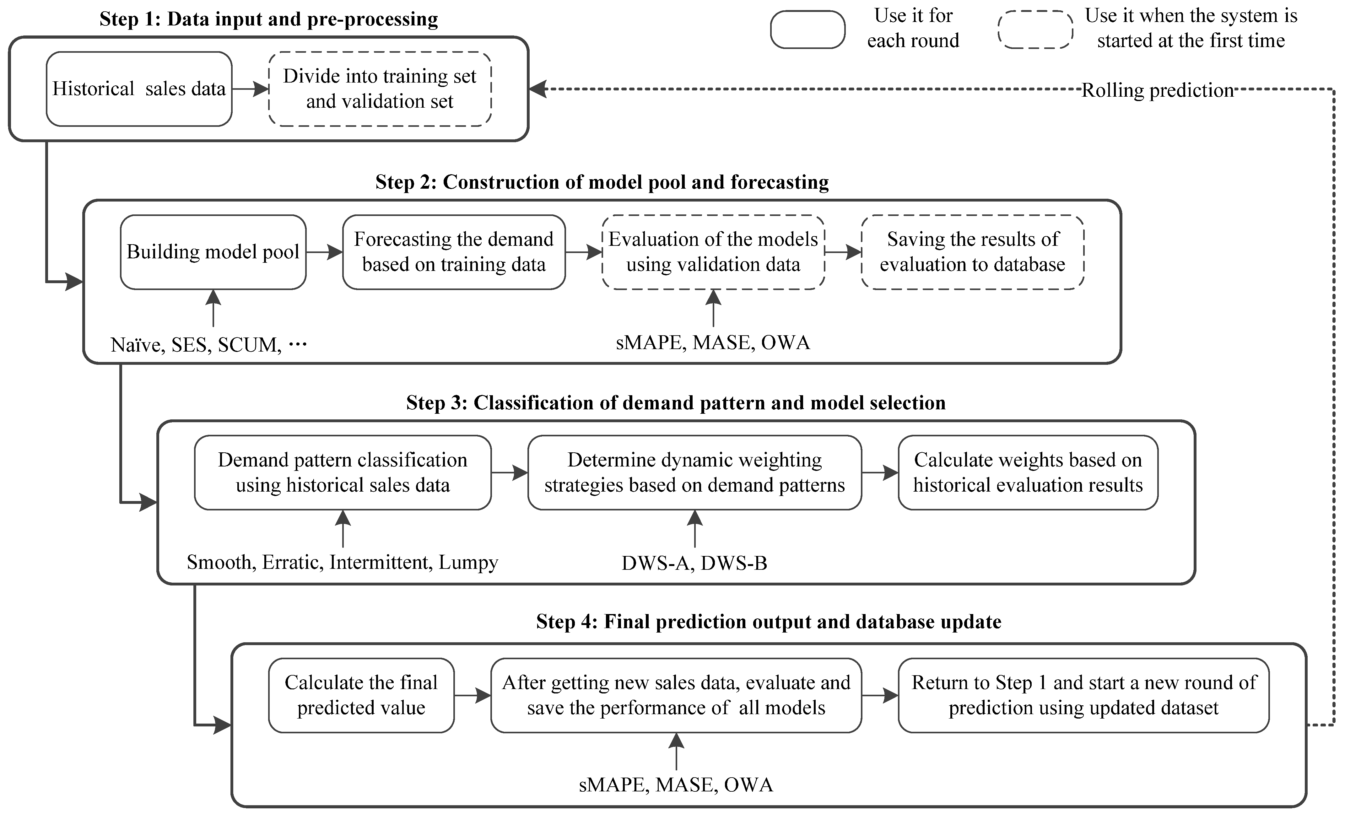
The existing literature indicates that the performance of forecasting models largely depends on the choice of error measures, the model used for comparison, the forecasting horizon, and the type of data. Zhang [27] argued that no single prediction model is applicable to all cases. For instance, Aburto and Weber [20] found that neural networks are superior to ARIMA models, and the proposed additive hybrid approach yields the best results. Lee, Chen, Chen, Chen, and Liu [18] found that logistic regression performed better than BPNN and moving average, and Kuo [28] found that the fuzzy neural network has better performance than conventional statistical methods. Thus, which forecasting techniques should be chosen when retailers face complex environments in production operations and management?

Since no single model always outperforms other candidate models in all cases, it is necessary to find a model selection method for any given SKU or item. Recently, some scholars have paid more attention to the topic of forecasting model selection.

Table 1. Review of published literature for forecasting model selection.

Article	Model Selection Strategy	Model Selection Criteria	Candidate Model
Fildes [29]	Aggregate selection	Out-of-sample performance	Filter model; Robust Trend Estimation
Taghiyeh, Lengacher, and Handfield [30]	Individual selection	In-sample performance. Out-of-sample performance	Naïve; Exponential Smoothing Models; ARIMA; Theta
Villegas, Pedregal, and Trapero [31]	Individual selection	Information criteria. In-sample performance	White Noise; Moving Average; Simple Exponential Smoothing; Mean; Median
Ulrich, Jahnke, Langrock, Pesch, and Senge [4]	Individual selection	Feature-based	Linear Regression; Generalized Additive Models; Quantile Regression; ARIMAX
Our study	Individual selection. Combination forecasts	Feature-based. Out-of-sample performance	Benchmark and winning models in M-Competitions

shows typical papers that have investigated forecasting model selection and presents the contribution of our study to the literature. The strategies for selecting the best prediction model according to the historical performance of candidate models can be classified into three types: individual selection, aggregate selection, and combination forecasts. Individual selection refers to finding the most suitable prediction model for each SKU or item. Instead, aggregate selection refers to when a single forecasting model is used for all SKUs or items [29]. Combined forecasts combine a set of forecasting models by building a weight coefficient vector. Individual model selection is more effective than most aggregation model selection methods, but the former has the disadvantage of higher complexity and computational costs [30]. In the individual selection procedure, information criteria (such as Akaike information), time series features, in-sample performance, and out-of-sample performance are usually used as model selection criteria. For instance, Villegas et al. [31] proposed a model selection method that combines information criteria and in-sample performance using a support vector machine. Taghiyeh, Lengacher, and Handfield [30] developed an approach that combines both in-sample and out-of-sample performance. Ulrich, Jahnke, Langrock, Pesch, and Senge [4] considered model selection as a classification problem and proposed a model selection framework via classification based on the labeled training data. Combining different models is another effective way to improve the performance of prediction [27]. However, Claeskens, Magnus, Vasnev, and Wang [3] showed that simple weighting schemes, such as arithmetic mean, usually produce equally good or better predictions than more complex weighting schemes.

The contribution of our study is to determine the corresponding model selection strategies that combine individual selection and combination forecasts based on both the demand patterns and the out-of-sample performance for each item. Further, we selected the benchmark and winning models in M-Competitions as the candidate models.

3. Methodology

In this section, we designed an automatic forecasting system to address model selection of sales forecasting in the retail industry. Figure 1 shows the flowchart of the system framework, which was designed to include four steps: data input and pre-processing, construction of model pool and forecasting, classification of demand pattern and model selection, and final prediction output and database update.

3.1. Design of Forecasting Model Pool

According to Figure 1, we know that the sales characteristics of different items vary greatly. Moreover, the sales characteristics of each item will also change over time. Therefore, no single forecasting method can maintain the advantage in the demand forecasting of all items. In this study, the idea of dynamic optimization is introduced into the task of forecasting. Firstly, a model pool composed of multiple prediction methods was constructed. Secondly, a vector of dynamic weight coefficients was determined based on the performance of the prediction methods in practice. Finally, the prediction of each item was determined according to the corresponding demand pattern and weight vector of the item.

Based on M-Competitions, this study selected the nine most popular forecasting models to build a pool of models for predicting sales of retail products.

Sub-Model 1: Naïve. The value of the last sales is simply used for all forecasts.

Sub-Model 2: Seasonal Naïve. Considering the sales characteristics of retail products, the model uses daily sales for the previous week as the forecast for the same day of the week.

Sub-Model 3: Single exponential smoothing (SES). The SES model weights the sum of the predicted and actual values of historical sales through the smoothing coefficient.

Sub-Model 4: Holt’s linear exponential smoothing. The Holt model considers the linear trend of the sequence on the basis of the SES model [11].

Sub-Model 5: Dampened trend exponential smoothing. The damped model considers the damping trend on the basis of the Holt model [32].

Sub-Model 6: Comb S-H-D. The ‘Comb S-H-D’ method is the simple arithmetic average of Models 3, 4, and 5. The Comb S-H-D model is more accurate than the three individual methods in M3 competition [25].

Sub-Model 7: Theta. The theta model decomposes the time series into two or more curves, which are combined by theta coefficients [33].

Sub-Model 8: 4Theta. The 4Theta model takes into account the nonlinear pattern of trend and the strength of adjustment trend on the basis of the theta model, and introduces a multiplication term into the model [34].

Sub-Model 9: Simple combination of univariate model. The SCUM model combines four methods: exponential smoothing, complex exponential smoothing, ARIMA, and dynamic optimization theta, and takes the median of the predicted values of the four models as the final predicted value [35]. The SCUM model outperformed most models and improved by 5.6% compared with the benchmark model in M4 competition [8].

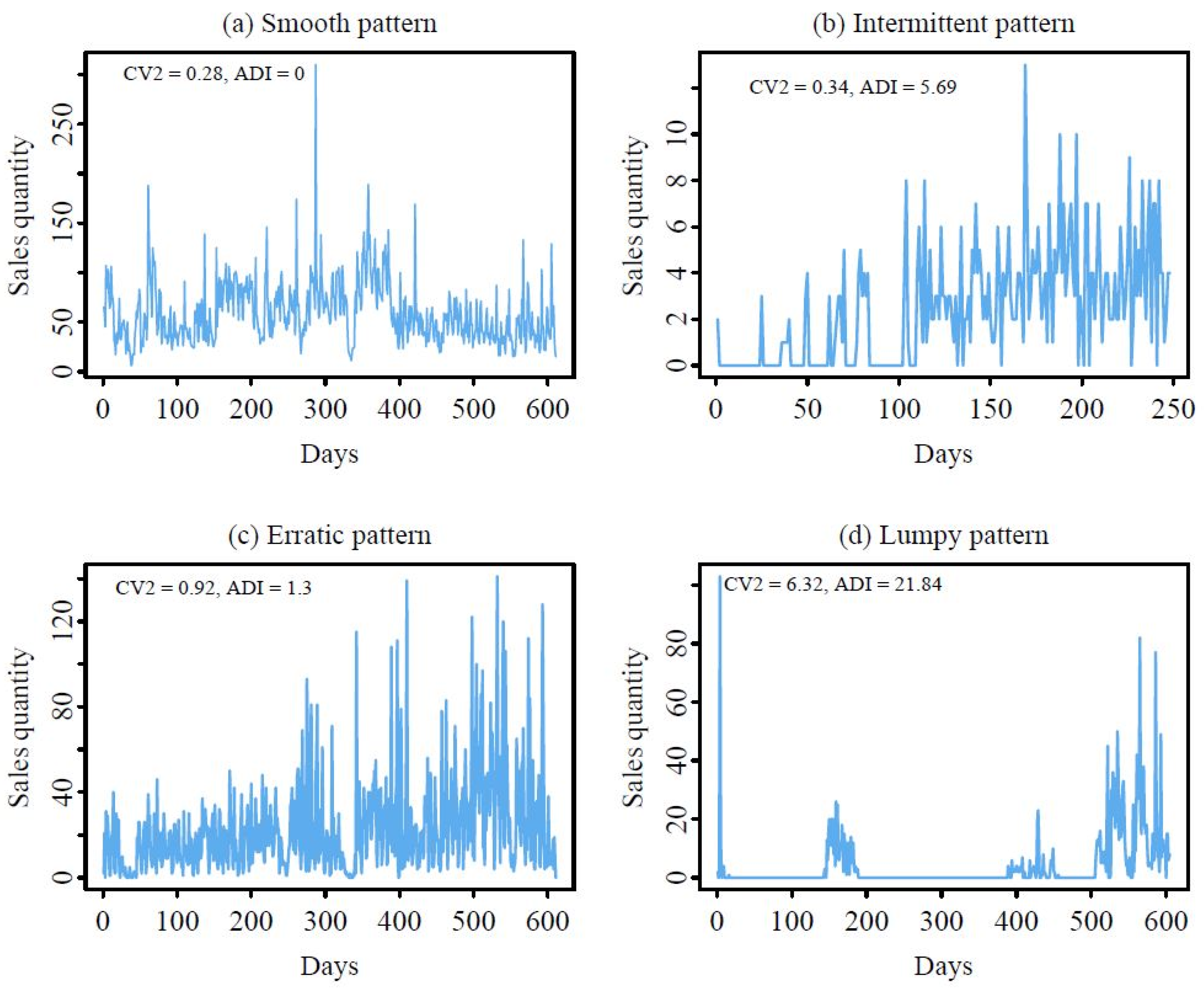
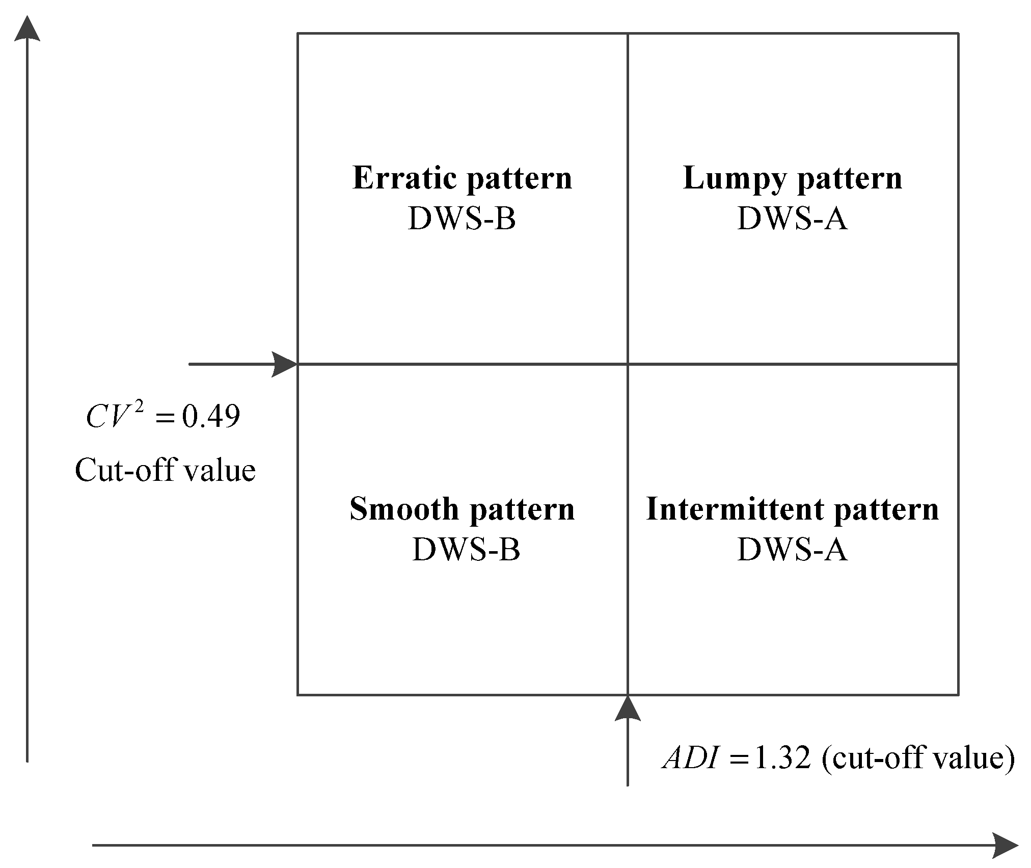
3.2. Demand Pattern Classification

For retail stores, the sales characteristics of different items vary greatly. The coefficient of variation is an effective index to measure the volatility of an item’s demand, which is defined by the ratio of the standard deviation to the mean demand. The squared coefficient of variation (CV²) of the demand sizes is given by:

$$\begin{array}{l}{\mathrm{CV}}^2=\frac{{\sigma }^2}{{\mu }^2}\\ \end{array}$$

(1)

The demand for some products may be zero in some time periods. The average inter-demand interval (ADI) is another important indicator to describe the demand characteristics of items. The ADI is calculated as follows:

$$\mathrm{ADI}=\frac{Z}{I}$$

(2)

where $Z$ is the number of zero demand, and $I$ is the number of intervals. For example, the daily demand of an item is [3,0,2,0,0,3,0,1,0,4], and then the average inter-demand interval is 5/4.

Based on the series’ average inter-demand interval and the squared coefficient of variation of the demand sizes, Syntetos et al. [36] proposes a rule to classify demand patterns into four categories: smooth (CV² < 0.49 and ADI < 1.32), intermittent (CV² < 0.49 and ADI ≥ 1.32), erratic (CV² ≥ 0.49 and ADI < 1.32), and lumpy (CV² ≥ 0.49 and ADI ≥ 1.32).

Figure 2 shows an example of four items selling on JD, a large B2C online retailer in China. According to CV² and ADI, these four items represent the sales characteristics of the four demand patterns, respectively. The smooth pattern is characterized by relatively stable demand volatility and a short average inter-demand interval. The lumpy pattern is characterized by high demand volatility and a long average inter-demand interval. Obviously, the demand prediction of the lumpy pattern will be more difficult than that of the smooth pattern.

3.3. Design of Dynamic Weighting Strategy

Suppose that the model pool $M$ has $m$ sub-models. The sub-model $i$ predicts the demand ${\widehat{y}}_{i,T+1}$ at $T+1$ based on the historical observations $y=\{y_1,\dots ,y_T\}$.

$${\widehat{y}}_{i,T+1}=f_i(y|y_1,\dots ,y_T), i\in M$$

(3)

Let $w=[w_1,\dots ,w_m]$ present a weight vector. The objective of the ensemble model is to determine the weight coefficient of each sub-model ($w_i$) and to obtain the final prediction value by weighted summation of the output of the sub-model.

$${\widehat{Y}}_{T+1}={\displaystyle \sum _{i=1}^m{w}_{i,T+1}}{\widehat{y}}_{i,T+1},w_{i,T+1}=[0,1],{\displaystyle \sum w_{i,T+1}}=1$$

(4)

The weight coefficient will change with the performance of the model in multi-round rolling prediction. $e_{i,t}$ denotes the error metric of model $i$ at $t$, such as the root mean square error or symmetric mean absolute percentage error, and $E_{i,k}$ represents the performance of model $i$ over a period of time:

$$E_{i,k}=\frac{1}{k}{\displaystyle \sum _{t=T+1}^{T+k}{e}_{i,t}},t=\{T+1,T+2,\dots ,T+k\}$$

(5)

Based on the performance of the sub-models in reality, this study proposes two dynamic weighting strategies.

Dynamic weighting strategy A (DWS-A): The final predictions of DWS-A are the forecasts of that model, which outperforms other models on historical data. The weight coefficient of sub-model $i$ under the DWS-A is as follows:

$$w_{i,k}^A=\left\{\begin{array}{l}1,if E_{i,k}=\min \left\{E_k\right\},\\ 0, \mathrm{otherwise}.\end{array}\right.$$

(6)

where $E_k=\{E_{1,k},\dots ,E_{i,k},\dots ,E_{m,k}\}$ is the set of error metrics of all sub-models.

Dynamic weighting strategy B (DWS-B): The final predictions of DWS-A utilize all the sub-models, which are weighted according to their performance on historical data. The weight coefficient of sub-model $i$ under the DWS-B is given by the formula:

$$w_{i,k}^B=\frac{\max \left\{E_k\right\}-E_{i,k}}{{\displaystyle {\sum }_{i=1}^m(\max \{E_k\}-E_{i,k})}}$$

(7)

In the real world, the value of error metrics will change dynamically as the models roll forward. Thus, the weight coefficients ($w_{i,k}^A$ and $w_{i,k}^B$) will also change with $k$. The final predictions of DWS-A and DWS-B at $T+k+1$ are given by the formula:

$${\widehat{Y}}_{T+k+1}^j={\displaystyle \sum _{i=1}^m{w}_{i,k}^j}{\widehat{y}}_{i,T+k+1},j\in \{A,B\}$$

(8)

3.4. Model Evaluation

Cross-validation is a primary method of measuring the predictive performance of a model. In this study, symmetric mean absolute percentage error (sMAPE), mean absolute scaled error (MASE), and overall weighted average (OWA) were used to evaluate the performance of the forecasting methods [8,25,37]. The sMAPE is defined as:

$$\mathrm{sMAPE}=\frac{1}{h}{\displaystyle {\sum }_{t=1}^h\frac{2|y_t-{\widehat{y}}_t|}{\left|y_t\right|+\left|{\widehat{y}}_t\right|}}.$$

(9)

where $y_t$ is the real sales at point $t$, ${\widehat{y}}_t$ is the forecasting sales, and $h$ is the forecasting horizon. Items with intermittent demand and lumpy demand are very common in retailing. The problem of large error can be avoided by using symmetric MAPE when the actual values, $y_t$, are close to zero.

The MASE is defined as:

$$\mathrm{MASE}=\frac{1}{h}\frac{{\displaystyle {\sum }_{t=1}^h|y_t-{\widehat{y}}_t|}}{\frac{1}{n-r}{\displaystyle {\sum }_{t=r+1}^n|y_t-y_{t-r}|}}$$

(10)

where $r$ is the frequency of the data and $n$ is the number of historical observations. The MASE is a scale-free error metric. It never yields undefined or infinite values and therefore is a good choice for intermittent demand and lumpy demand.

The OWA is computed by averaging the relative MASE and the relative sMAPE for all samples. The OWA is defined as:

$${\mathrm{OWA}}_i=\frac{1}{2}\left(\frac{{\displaystyle {\sum }_1^s{\mathrm{sMAPE}}_i}}{{\displaystyle {\sum }_1^s{\mathrm{sMAPE}}_1}}+\frac{{\displaystyle {\sum }_1^s{\mathrm{MASE}}_i}}{{\displaystyle {\sum }_1^s{\mathrm{MASE}}_1}}\right),i\in M$$

(11)

where ${\mathrm{OWA}}_i$ is the OWA of method $i$, $s$ is the number of series, and ${\mathrm{sMAPE}}_1$ and ${\mathrm{MASE}}_1$ are the performance measures of Naïve. The OWA is an effective metric to compare the performance difference between proposed models and the benchmark model. If the OWA of the proposed model is lower than 1, it means that the proposed model outperformed the benchmark model, and vice versa.

4. Empirical Analysis

4.1. Empirical Data

We demonstrate the applicability of the sales forecasting methods using two real-world problems. The first dataset was taken from Haolinju, a large chain of a convenience store in Beijing, China. Haolinju has more than 800 stores and typically stocks more than 5000 different items in its distribution center. Haolinju’s sales data ranges from 9 July 2016 to 8 July 2018 and contains 5383 items of different categories and various time horizons. The second dataset was taken from JD, also known as Jingdong, a large B2C online retailer in China. JD’s sales data ranges from 1 January 2016 to 31 December 2017 and contains 1000 items of different categories and various time horizons. It should be noted that JD’s data in June and November are excluded due to promotional activities. Since some forecasting methods require historical data for training, we removed items with sales records less than 40 days. Then, there were 4027 items in Haolinju’s data and 936 items in JD’s data that met the requirements.

According to the indicators of CV² and ADI, those items in both retailers were divided into four demand patterns: smooth, intermittent, erratic, and lumpy.

Table 2. Characteristics of the sales of the offline retailer (Haolinju) and the online retailer (JD).

Characteristics	Haolinju	JD
Total items
No. of series	4027	936
Mean obs./series	535.0	209.4
Smooth pattern
No. of series	1336 (33.2%)	34 (3.6%)
% Zero values	0.3 (2.2)	2.1 (4.5)
Average of nonzero demand	471.4 (1155.5)	49.8 (50.9)
CV2 of nonzero demand	0.223 (0.128)	0.376 (0.084)
ADI	0.096 (0.302)	0.607 (0.554)
Intermittent pattern
No. of series	713 (17.7%)	40 (4.3%)
% Zero values	56.8 (25.5)	12.4 (14.9)
Average of nonzero demand	38.7 (172.7)	45.6 (121.6)
CV2 of nonzero demand	0.315 (0.109)	0.403 (0.059)
ADI	6.949 (17.059)	3.739 (3.986)
Erratic pattern
No. of series	767 (19.0%)	162 (17.3%)
% Zero values	1.1 (3.4)	2.9 (4.7)
Average of nonzero demand	295.4 (667.4)	91.7 (171.1)
CV2 of nonzero demand	2.340 (4.124)	2.641 (6.377)
ADI	0.290 (0.476)	0.781 (0.518)
Lumpy pattern
No. of series	1211 (30.1%)	700 (74.8%)
% Zero values	45.8 (23.5)	21.9 (18.4)
Average of nonzero demand	34.0 (189.5)	42.3 (102.1)
CV2 of nonzero demand	1.586 (3.023)	3.408 (7.795)
ADI	7.096 (36.012)	3.862 (6.421)

ADI: average demand interval; CV: the coefficient of variation. Means (standard deviation) are presented in the table.

shows the detailed descriptive statistics of CV² and ADI on those four demand patterns. There were 1336 (33.2%) items in Haolinju’s data and 34 (3.6%) items in JD’s data that met the smooth demand pattern. The CV² of nonzero demand of Haolinju and JD was 0.223 and 0.376, respectively, and the ADI of both retailers was 0.096 and 0.607, respectively. There were 1211 (30.1%) items in Haolinju’s data and 700 (74.8%) items in JD’s data that met the lumpy demand pattern. The CV² of nonzero demand of Haolinju and JD was 1.586 and 3.408, respectively, and the ADI of Haolinju and JD was 7.096 and 3.862, respectively. In the lumpy pattern, the sales volatility of Haolinju was less than JD, but the former had a longer demand interval.

4.2. Empirical Results

Based on the two datasets drawn from an offline retailer and an online retailer, we examined the performance of two dynamic weighting strategies by comparing with benchmark models such as Naïve, Comb S-H-D, and SCUM. We implemented multi-round rolling forecast with different horizons. The last 10 days of each series were used to test the performance of the models. We conducted the experiment with ten rounds and one horizon for short-term forecasting, and the experiment with four rounds and seven horizons for long-term forecasting. For example, suppose 1 item has 40 days of sales data, and we set the forecasting horizon equal to 1. Before starting the forecasting system, we used the sales data from day 1 to day 29 to train the sub-models and forecast the demand on day 30. In round 1, based on the performance of each sub-model on day 30, the sales data of the first 30 days were used to predict the demand on day 31. In round 10, the sales data of the first 39 days were used to forecast the demand on day 40. In this study, we measured the performance of the proposed methods with Windows 10, Intel(R) Core(TM) i7-8550U CPU @ 1.80 GHz, 8.00 GB RAM. The forecasting process was performed by using R Studio Version 4.0.5. The performances of two dynamic weighting strategies in four demand patterns were analyzed, respectively.

4.2.1. Smooth Pattern

The forecast accuracy comparisons for different methods with different forecasting horizons in the smooth pattern are shown in

Table 3. The performance of the five methods for rolling forecast testing in the smooth pattern.

Model	sMAPE	MASE	OWA	% Improvement of Method over the Naïve
Haolinju: Horizon = 1 (Obs. = 1336 × 1 × 10) a
Naïve	19.948 (1.991)	0.801 (0.152)	1.000 (0.000)	-
Comb S-H-D	17.366 (1.812)	0.707 (0.126)	0.883 (0.076)	11.7%
SCUM	17.714 (1.966)	0.696 (0.128)	0.885 (0.070)	11.5%
DWS-A	18.594 (1.961)	0.763 (0.135)	0.942 (0.069)	5.8%
DWS-B	17.387 (1.972)	0.701 (0.133)	0.873 (0.071)	12.7%
Haolinju: Horizon = 7 (Obs. = 1336 × 7 × 4) b
Naïve	22.114 (0.967)	0.926 (0.054)	1.000 (0.000)	-
Comb S-H-D	18.749 (0.135)	0.811 (0.009)	0.863 (0.043)	13.7%
SCUM	18.947 (0.216)	0.796 (0.008)	0.861 (0.043)	13.9%
DWS-A	17.588 (0.158)	0.768 (0.020)	0.813 (0.036)	18.7%
DWS-B	17.797 (0.334)	0.764 (0.010)	0.816 (0.038)	18.4%
JD: Horizon = 1 (Obs. = 34 × 1 × 10) b
Naïve	49.071 (8.709)	0.975 (0.161)	1.000 (0.000)	-
Comb S-H-D	42.648 (9.694)	0.876 (0.158)	0.897 (0.129)	10.3%
SCUM	41.644 (9.287)	0.845 (0.144))	0.871 (0.119)	12.9%
DWS-A	45.632 (6.064)	0.933 (0.234)	0.975 (0.140)	2.5%
DWS-B	40.476 (8.104)	0.819 (0.160)	0.858 (0.118)	14.2%
JD: Horizon = 7 (Obs. = 34 × 7 × 4) b
Naïve	52.739 (3.593)	1.075 (0.121)	1.000 (0.000)	-
Comb S-H-D	41.531 (0.594)	0.903 (0.027)	0.841 (0.055)	25.9%
SCUM	40.942 (0.657)	0.877 (0.024)	0.821 (0.050)	27.9%
DWS-A	38.658 (1.515)	0.838 (0.009)	0.789 (0.033)	31.1%
DWS-B	38.707 (0.387)	0.823 (0.004)	0.782 (0.782)	31.8%

^a The Comb S-H-D outperformed the other sub-models in this dataset. ^b The SCUM outperformed the other sub-models in these datasets.

. The Comb S-H-D outperformed the other eight methods in the model pool for Haolinju’s data when the horizon was equal to one. In the remaining three datasets, the SCUM outperformed the other eight sub-models. Surprisingly, the DWS-B outperformed all sub-models on all datasets, and the DWS-A performed better than all sub-models for Haolinju’s data and JD’s data when the horizon was equal to seven. For instance, for Haolinju’s data when the horizon was equal to seven, the sMAPE of Naïve was 22.114%, that of Comb S-H-D was 18.749%, that of SCUM was 18.947%, while for DWS-A and DWS-B they were 17.588% and 17.387%, respectively. We also calculated the improvement in OWA of the Comb S-H-D, the SCUM, and the two proposed dynamic weighting strategies over the Naïve. According to OWA, for Haolinju’s data when the horizon was equal to seven, the DWS-B was 18.4% more accurate than the Naïve and 5.23% more than the SCUM. In general, the forecast results in the smooth pattern indicate that the proposed DWS-B performed better than the DWS-A method and the other three benchmark models.

4.2.2. Intermittent Pattern

The pattern of intermittent demand is characterized by a long average inter-demand interval and a low coefficient of variation. The results of

Table 4. The performance of the five methods for rolling forecast testing in the intermittent pattern.

Model	sMAPE	MASE	OWA	% Improvement of Method over the Naïve
Haolinju: Horizon = 1 (Obs. = 713 × 1 × 10) a
Naïve	78.516 (3.403)	1.401 (0.142)	1.000 (0.000)	-
Comb S-H-D	123.704 (2.298)	1.257 (0.088)	1.241 (0.068)	−24.1%
SCUM	125.214 (2.144)	1.249 (0.091)	1.248 (0.066)	−24.8%
DWS-A	79.247 (3.445)	1.349 (0.097)	0.989 (0.035)	1.1%
DWS-B	111.481 (13.306)	1.254 (0.090)	1.164 (0.127)	-16.4%
Haolinju: Horizon = 7 (Obs. = 713 × 7 × 4) b
Naïve	82.682 (3.055)	1.532 (0.127)	1.000 (0.000)	-
Comb S-H-D	124.918 (0.553)	1.315 (0.017)	1.175 (0.061)	−17.5%
SCUM	126.654 (0.344)	1.302 (0.016)	1.181 (0.063)	−18.1%
DWS-A	75.052 (1.303)	1.361 (0.071)	0.889 (0.029)	11.1%
DWS-B	120.953 (1.360)	1.295 (0.029)	1.146 (0.061)	−14.6%
JD: Horizon = 1 (Obs. = 40 × 1 × 10) a
Naïve	49.867 (7.385)	1.094 (0.139)	1.000 (0.000)	-
Comb S-H-D	52.398 (9.005)	1.057 (0.167)	1.025 (0.193)	−2.5%
SCUM	55.184 (8.113)	1.037 (0.162)	1.046 (0.171)	−4.6%
DWS-A	47.535 (7.858)	1.050 (0.157)	0.960 (0.106)	4.0%
DWS-B	48.858 (7.067)	0.994 (0.160)	0.949 (0.118)	5.1%
JD: Horizon = 7 (Obs. = 40 × 7 × 4) c
Naïve	56.265 (5.720)	1.251 (0.044)	1.000 (0.000)	-
Comb S-H-D	55.036 (1.417)	1.157 (0.037)	0.955 (0.083)	4.5%
SCUM	57.666 (0.224)	1.135 (0.038)	0.974 (0.077)	2.6%
DWS-A	47.379 (0.724)	1.058 (0.051)	0.857 (0.074)	14.3%
DWS-B	52.147 (1.313)	1.062 (0.020)	0.903 (0.084)	9.7%

^a The Naïve outperformed the other sub-models in these datasets. ^b The sNaïve outperformed the other sub-models in this dataset (OWA = 0.956). ^c The 4Theta outperformed the other sub-models in this dataset (OWA = 0.940).

show that the Naïve model provided more accuracy than all other sub-models for Haolinju’s data and JD’s data when the horizon was equal to one. This means that forecasting intermittent demand is not an easy task. However, the DWS-A outperformed all sub-models for Haolinju’s data and JD’s data. For instance, for Haolinju’s data when the horizon was equal to seven, the sMAPE of Naïve was 82.682%, that of Comb S-H-D was 124.918%, that of SCUM was 126.654%, while for DWS-A it was 75.052%. According to OWA for Haolinju’s data when the horizon was equal to seven, the DWS-A was 11.1% more accurate than the Naïve and 7% more than the best sub-model, sNaïve.

4.2.3. Erratic Pattern

The pattern of erratic demand is characterized by a short average inter-demand interval and a high coefficient of variation. The results of

Table 5. The performance of the five methods for rolling forecast testing in the erratic pattern.

Model	sMAPE	MASE	OWA	% Improvement of Method over the Naïve
Haolinju: Horizon = 1 (Obs. = 767 × 1 × 10) a
Naïve	32.220 (2.656)	0.978 (0.686)	1.000 (0.000)	-
Comb S-H-D	31.539 (1.565)	0.975 (0.670)	1.007 (0.127)	−0.7%
SCUM	29.752 (1.562)	0.934 (0.667)	0.956 (0.119)	4.4%
DWS-A	30.604 (2.485)	0.976 (0.713)	0.958 (0.116)	4.2%
DWS-B	28.731 (1.563)	0.945 (0.720)	0.915 (0.089)	8.5%
Haolinju: Horizon = 7 (Obs. = 767 × 7 × 4) a
Naïve	36.492 (1.616)	1.259 (0.293)	1.000 (0.000)	-
Comb S-H-D	35.613 (0.853)	1.332 (0.253)	1.025 (0.049)	−2.5%
SCUM	33.380 (0.660)	1.248 (0.208)	0.969 (0.093)	3.1%
DWS-A	30.258 (1.428)	1.058 (0.258)	0.841 (0.069)	15.9%
DWS-B	31.030 (0.656)	1.140 (0.326)	0.886 (0.048)	11.4%
JD: Horizon = 1 (Obs. = 162 × 1 × 10) b
Naïve	59.324 (8.485)	1.451 (0.597)	1.000 (0.000)	-
Comb S-H-D	63.360 (11.363)	1.407 (0.523)	1.046 (0.191)	−4.6%
SCUM	61.548 (10.980)	1.343 (0.511)	1.003 (0.171)	−0.3%
DWS-A	56.958 (6.653)	1.328 (0.482)	0.956 (0.093)	4.4%
DWS-B	56.821 (8.354)	1.298 (0.496)	0.942 (0.097)	5.8%
JD: Horizon = 7 (Obs. = 162 × 7 × 4) a
Naïve	63.030 (3.753)	1.431 (1.115)	1.000 (0.000)	-
Comb S-H-D	62.366 (1.894)	1.472 (0.070)	1.022 (0.027)	−2.2%
SCUM	60.903 (1.585)	1.409 (0.090)	0.983 (0.024)	1.7%
DWS-A	52.883 (2.642)	1.303 (0.889)	0.889 (0.020)	11.1%
DWS-B	54.516 (1.838)	1.294 (0.898)	0.898 (0.012)	10.2%

^a The SCUM outperformed the other sub-models in these datasets. ^b The Naïve outperformed the other sub-models in this dataset.

show that the DWS-B outperformed all sub-models for Haolinju’s data and JD’s data. For example, for Haolinju’s data when the horizon was equal to one, the sMAPE of Naïve was 32.220%, that of Comb S-H-D was 31.539%, that of SCUM was 29.752%, while for DWS-B it was 28.731%. According to OWA for Haolinju’s data, when the horizon was equal to one, the DWS-B was 8.5% more accurate than the Naïve and 4.29% than the best sub-model, SCUM.

4.2.4. Lumpy Pattern

The pattern of lumpy demand, which is characterized by a long average inter-demand interval and a high coefficient of variation, is a common phenomenon in online and offline retail. The results of

Table 6. The performance of the five methods for rolling forecast testing in the lumpy pattern.

Model	sMAPE	MASE	OWA	% Improvement of Method over the Naïve
Haolinju: Horizon = 1 (Obs. = 1211 × 1 × 10) a
Naïve	80.997 (3.429)	1.176 (0.158)	1.000 (0.000)	-
Comb S-H-D	108.250 (1.737)	1.072 (0.102)	1.127 (0.061)	−12.7%
SCUM	110.246 (1.581)	1.059 (0.103)	1.134 (0.062)	−13.4%
DWS-A	81.301 (3.306)	1.143 (0.141)	0.983 (0.014)	1.7%
DWS-B	98.551 (9.256)	1.078 (0.123)	1.065 (0.073)	−6.5%
Haolinju: Horizon = 1 (Obs. = 1211 × 7 × 4) a
Naïve	86.245 (0.944)	1.361 (0.112)	1.000 (0.000)	-
Comb S-H-D	110.943 (0.141)	1.207 (0.035)	1.078 (0.031)	−7.8%
SCUM	113.245 (0.468)	1.187 (0.034)	1.084 (0.031)	−8.4%
DWS-A	76.947 (0.515)	1.218 (0.026)	0.884 (0.033)	11.6%
DWS-B	106.015 (0.426)	1.178 (0.027)	1.038 (0.028)	−3.8%
JD: Horizon = 1 (Obs. = 700 × 1 × 10) b
Naïve	70.315 (4.558)	1.487 (0.368)	1.000 (0.000)	-
Comb S-H-D	72.850 (8.011)	1.384 (0.386)	0.987 (0.083)	1.3%
SCUM	73.208 (7.767)	1.352 (0.383)	0.980 (0.079)	2.0%
DWS-A	68.414 (4.737)	1.401 (0.348)	0.969 (0.042)	3.1%
DWS-B	68.991 (6.494)	1.316 (0.376)	0.941 (0.055)	5.9%
JD: Horizon = 7 (Obs. = 700 × 7 × 4) b
Naïve	75.817 (1.651)	1.549 (0.041)	1.000 (0.000)	-
Comb S-H-D	74.057 (0.600)	1.414 (0.079)	0.945 (0.031)	5.5%
SCUM	74.092 (0.707)	1.370 (0.075)	0.931 (0.030)	6.9%
DWS-A	64.56 (0.387)	1.341 (0.097)	0.853 (0.033)	14.7%
DWS-B	69.691 (0.719)	1.319 (0.085)	0.880 (0.029)	12.0%

^a The Naïve outperformed the other sub-models in these datasets. ^b The SCUM outperformed the other sub-models in these datasets.

show that the DWS-A provided more accuracy than all sub-models for Haolinju’s data and JD’s data. For example, for JD’s data when the horizon was equal to seven, the MASE of Naïve was 75.817%, that of Comb S-H-D was 74.057%, that of SCUM was 74.092%, while for DWS-A it was 64.560%. According to OWA for JD’s data, when the horizon was equal to seven, the DWS-A was 14.7% more accurate than the Naïve and 8.38% than the best sub-model, SCUM.

4.3. Optimal Dynamic Weighting Strategy for Each Demand Pattern

Based on the empirical analysis results, as shown in Figure 3, we can determine an optimal dynamic weighting strategy for each demand pattern. For items in the smooth or erratic pattern, it is recommended to use the DWS-B method to output the final predicted value. For items in the intermittent or lumpy pattern, it is recommended to use the DWS-A method to output the final predicted value. This means that for such items with intermittent or lumpy patterns, retailers only need to consider the output of the optimal sub-model as the final predictions.

5. Conclusions

In this paper, we proposed dynamic model selection based on demand pattern classification as a new approach in the retailing forecasting area. This approach offers a framework to address the challenge of model selection with complex demand patterns in retail practice. Based on a series’ average inter-demand interval and the squared coefficient of variation of the demand sizes, we divided the demand patterns of all items of retailers into four types: smooth, intermittent, erratic, and lumpy. Some studies have proposed specific prediction methods for certain demand patterns, such as Syntetos-Boylan Approximation and Croston methods for intermittent demand [38]. However, the demand pattern of items may change over time. Moreover, any single model for demand forecasting cannot be the most accurate in all periods of an item. It is necessary to monitor and update the demand pattern and switch appropriate forecasting methods. We first built a pool of models, including nine classical methods, in the M-Competitions. Then, we proposed two dynamic weighting strategies based on the historical performance of all candidate models, namely DWS-A and DWS-B. The DWS-A method only selects the best prediction model in the past as the final model. The DWS-B method sets different weights according to the historical performance of candidate models. The weights of both strategies change dynamically over time. This framework can provide automatic model selection for retail demand forecasting. Further, this approach has better interpretability and may be more acceptable to decision makers.

We verified the effectiveness of this approach by using two large datasets from an offline retailer and an online retailer in China. We implemented multi-round rolling forecast with different demand patterns and horizons to verify the generalization ability of this approach. The pattern of smooth demand, which is characterized by low volatility and short intervals, is easier to predict. For this pattern, the DWS-B delivered more accuracy at various forecast horizons. Additionally, the DWS-B in the pattern of erratic demand outperformed all models in the pool. This means that the combination forecast is more suitable for items with a short ADI. The demand patterns of intermittent and lumpy, which are characterized by a high proportion of zero values, are not easier to predict. However, the DWS-A still outperformed all models in the pool. This means that individual selection is more suitable for items with a long ADI. In general, the proposed dynamic weighting strategies dominated the benchmark and winning prediction models in M-Competitions, including Naïve, Comb S-H-D, and SCUM. We suggest that the DWS-A method is applicable to the items of intermittent and lumpy patterns, and the DWS-B method is applicable to the items of smooth and erratic patterns.

We did not consider additional prediction methods in the pool of models, such as deep learning methods, as several models take extra time in the calculation and have higher complexity, and their performance is not necessarily as good as statistical models [8]. However, the model pool and empirical results of this study are sufficient to prove the effectiveness of the proposed model selection approach. In future studies, additional models and factors that affect consumer demand should be included in this forecasting system to improve the forecast accuracy.

References

1. Simchi-Levi, D.; Wu, M.X. Powering retailers′ digitization through analytics and automation. Int. J. Prod. Res. 2018, 56, 809–816. [Google Scholar] [CrossRef]
2. Arunraj, N.S.; Ahrens, D. A hybrid seasonal autoregressive integrated moving average and quantile regression for daily food sales forecasting. Int. J. Prod. Econ. 2015, 170, 321–335. [Google Scholar] [CrossRef]
3. Claeskens, G.; Magnus, J.R.; Vasnev, A.L.; Wang, W. The forecast combination puzzle: A simple theoretical explanation. Int. J. Forecast. 2016, 32, 754–762. [Google Scholar] [CrossRef]
4. Ulrich, M.; Jahnke, H.; Langrock, R.; Pesch, R.; Senge, R. Classification-based model selection in retail demand forecasting. Int. J. Forecast. 2022, 38, 209–223. [Google Scholar] [CrossRef]
5. Makridakis, S.; Andersen, A.; Carbone, R.; Fildes, R.; Hibon, M.; Lewandowski, R.; Newton, J.; Parzen, E.; Winkler, R. The accuracy of extrapolation (time series) methods: Results of a forecasting competition. J. Forecast. 1982, 1, 111–153. [Google Scholar] [CrossRef]
6. Ching-Chin, C.; Ieng, A.I.K.; Ling-Ling, W.; Ling-Chieh, K. Designing a decision-support system for new product sales forecasting. Expert Syst. Appl. 2010, 37, 1654–1665. [Google Scholar] [CrossRef]
7. Neelamegham, R.; Chintagunta, P.K. Modeling and Forecasting the Sales of Technology Products. Qme-Quant. Mark. Econ. 2004, 2, 195–232. [Google Scholar] [CrossRef]
8. Makridakis, S.; Spiliotis, E.; Assimakopoulos, V. The M4 Competition: Results, findings, conclusion and way forward. Int. J. Forecast. 2018, 34, 802–808. [Google Scholar] [CrossRef]
9. Hyndman, R.J.; Athanasopoulos, G. Forecasting: Principles and Practice; OTexts: Melbourne, Australia, 2018. [Google Scholar]
10. Brown, R.G. Smoothing, Forecasting and Prediction of Discrete Time Series; Courier Corporation: Chelmsford, MA, USA, 2004. [Google Scholar]
11. Holt, C.C. Forecasting seasonals and trends by exponentially weighted moving averages. Int. J. Forecast. 2004, 20, 5–10. [Google Scholar] [CrossRef]
12. Winters, P.R. Forecasting sales by exponentially weighted moving averages. Manag. Sci. 1960, 6, 324–342. [Google Scholar] [CrossRef]
13. Box, G.E.; Jenkins, G.M.; Reinsel, G.C.; Ljung, G.M. Time Series Analysis: Forecasting and Control; John Wiley & Sons: Hoboken, NJ, USA, 2015. [Google Scholar]
14. Ali, Ö.G.; Sayın, S.; van Woensel, T.; Fransoo, J. SKU demand forecasting in the presence of promotions. Expert Syst. Appl. 2009, 36, 12340–12348. [Google Scholar] [CrossRef]
15. Peng, B.; Song, H.; Crouch, G.I. A meta-analysis of international tourism demand forecasting and implications for practice. Tour. Manag. 2014, 45, 181–193. [Google Scholar] [CrossRef]
16. Divakar, S.; Ratchford, B.T.; Shankar, V. Practice Prize Article—CHAN4CAST: A Multichannel, Multiregion Sales Forecasting Model and Decision Support System for Consumer Packaged Goods. Mark. Sci. 2005, 24, 334–350. [Google Scholar] [CrossRef]
17. Kong, J.; Martin, G. A backpropagation neural network for sales forecasting. In Proceedings of Proceedings of ICNN′95-International Conference on Neural Networks, Perth, Australia, 27 November 1995; pp. 1007–1011.
18. Lee, W.-I.; Chen, C.-W.; Chen, K.-H.; Chen, T.-H.; Liu, C.-C. Comparative study on the forecast of fresh food sales using logistic regression, moving average and BPNN methods. J. Mar. Sci. Technol. 2012, 20, 142–152. [Google Scholar] [CrossRef]
19. Chen, F.; Ou, T. Gray relation analysis and multilayer functional link network sales forecasting model for perishable food in convenience store. Expert Syst. Appl. 2009, 36, 7054–7063. [Google Scholar] [CrossRef]
20. Aburto, L.; Weber, R. Improved supply chain management based on hybrid demand forecasts. Appl. Soft Comput. 2007, 7, 136–144. [Google Scholar] [CrossRef]
21. Liu, J.; Liu, C.; Zhang, L.; Xu, Y. Research on sales information prediction system of e-commerce enterprises based on time series model. Inf. Syst. E-Bus. Manag. 2019, 18, 1–14. [Google Scholar] [CrossRef]
22. Rubio, L.; Alba, K. Forecasting Selected Colombian Shares Using a Hybrid ARIMA-SVR Model. Mathematics 2022, 10, 2181. [Google Scholar] [CrossRef]
23. Wang, C.-C.; Chang, H.-T.; Chien, C.-H. Hybrid LSTM-ARMA Demand-Forecasting Model Based on Error Compensation for Integrated Circuit Tray Manufacturing. Mathematics 2022, 10, 2158. [Google Scholar] [CrossRef]
24. Armstrong, J.S. Combining forecasts. In Principles of forecasting; Springer: Berlin/Heidelberg, Germany, 2001; pp. 417–439. [Google Scholar]
25. Makridakis, S.; Hibon, M. The M3-Competition: Results, conclusions and implications. Int. J. Forecast. 2000, 16, 451–476. [Google Scholar] [CrossRef]
26. Aye, G.C.; Balcilar, M.; Gupta, R.; Majumdar, A. Forecasting aggregate retail sales: The case of South Africa. Int. J. Prod. Econ. 2015, 160, 66–79. [Google Scholar] [CrossRef]
27. Zhang, G.P. Time series forecasting using a hybrid ARIMA and neural network model. Neurocomputing 2003, 50, 159–175. [Google Scholar] [CrossRef]
28. Kuo, R. A sales forecasting system based on fuzzy neural network with initial weights generated by genetic algorithm. Eur. J. Oper. Res. 2001, 129, 496–517. [Google Scholar] [CrossRef]
29. Fildes, R. Evaluation of Aggregate and Individual Forecast Method Selection Rules. Manag. Sci. 1989, 35, 1056–1065. [Google Scholar] [CrossRef]
30. Taghiyeh, S.; Lengacher, D.C.; Handfield, R.B. Forecasting model selection using intermediate classification: Application to MonarchFx corporation. Expert Syst. Appl. 2020, 151, 113371. [Google Scholar] [CrossRef]
31. Villegas, M.A.; Pedregal, D.J.; Trapero, J.R. A support vector machine for model selection in demand forecasting applications. Comput. Ind. Eng. 2018, 121, 1–7. [Google Scholar] [CrossRef]
32. Gardner, E.S.; Mckenzie, E. Forecasting Trends in Time Series. Manag. Sci. 1985, 31, 1237–1246. [Google Scholar] [CrossRef]
33. Assimakopoulos, V.; Nikolopoulos, K. The theta model: A decomposition approach to forecasting. Int. J. Forecast. 2000, 16, 521–530. [Google Scholar] [CrossRef]
34. Spiliotis, E.; Assimakopoulos, V. 4Theta: Generalizing the Theta Method for Automatic Forecasting. Available online: https://github.com/M4Competition/M4-methods (accessed on 1 July 2022).
35. Petropoulos, F.; Svetunkov, I. A simple combination of univariate models. Int. J. Forecast. 2020, 36, 110–115. [Google Scholar] [CrossRef]
36. Syntetos, A.A.; Boylan, J.E.; Croston, J.D. On the categorization of demand patterns. J. Oper. Res. Soc. 2005, 56, 495–503. [Google Scholar] [CrossRef]
37. Hyndman, R.J.; Koehler, A.B. Another look at measures of forecast accuracy. Int. J. Forecast. 2006, 22, 679–688. [Google Scholar] [CrossRef]
38. Tian, X.; Wang, H. Forecasting intermittent demand for inventory management by retailers: A new approach. J. Retail. Consum. Serv. 2021, 62, 102662. [Google Scholar] [CrossRef]
Figure 1. The system framework flowchart.
Mathematics 10 03179 g001
Figure 2. Typical sales characteristics of retail products of the four demand patterns.
Mathematics 10 03179 g002
Figure 3. Optimal dynamic weighting strategies in the four demand patterns.
Mathematics 10 03179 g003