

Deep Reinforcement Learning-Based RMSA Policy Distillation for Elastic Optical Networks

Abstract
:1. Introduction
2. Related Work
2.1. Deep Reinforcement Learning in RMSA of EONs
2.2. Transfer Learning in EONs
3. Preliminaries
3.1. Reinforcement Learning
3.2. Asynchronous Advantage Actor–Critic
4. Policy Distillation Design with EONs
4.1. Elastic Optical Networks
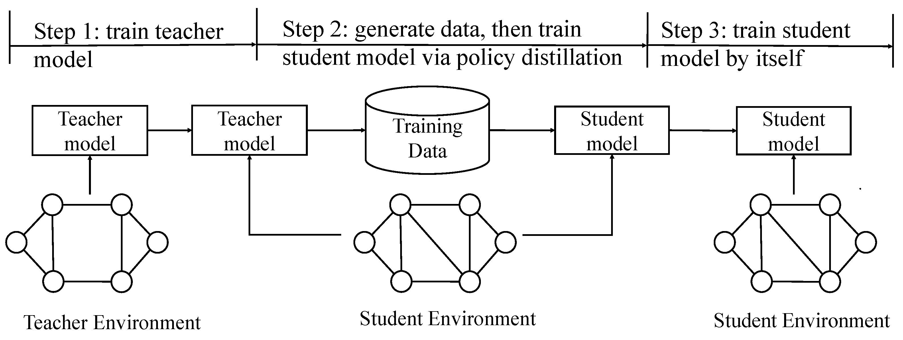
4.2. Policy Distillation Scheme
- Step 1: Train the teacher model. It is trained by interacting with the teacher environment.
- Step 2: Distill the knowledge from the teacher model and transfer the knowledge to the student model. The training data of the student model are generated by calling the well-trained teacher model obtained in Step 1, and then the student model is trained by fitting these data.
- Step 3: Train the student model by itself. After the training in Step 2, the student model will be further updated by interacting with student environment and no longer rely on the knowledge distilled from the teacher model.
4.3. State, Action, and Reward
- Starting index of the first available FS-block;
- Size of the first available FS-block;
- Number of required FSs;
- Average size of the available FS-block;
- Total number of available FSs.
4.4. Teacher Model
| Algorithm 1 Training algorithm of the teacher model. |
|
4.5. Student Model
| Algorithm 2 Training algorithm of student model. |
|
5. Performance Evaluation
5.1. Parameter Settings
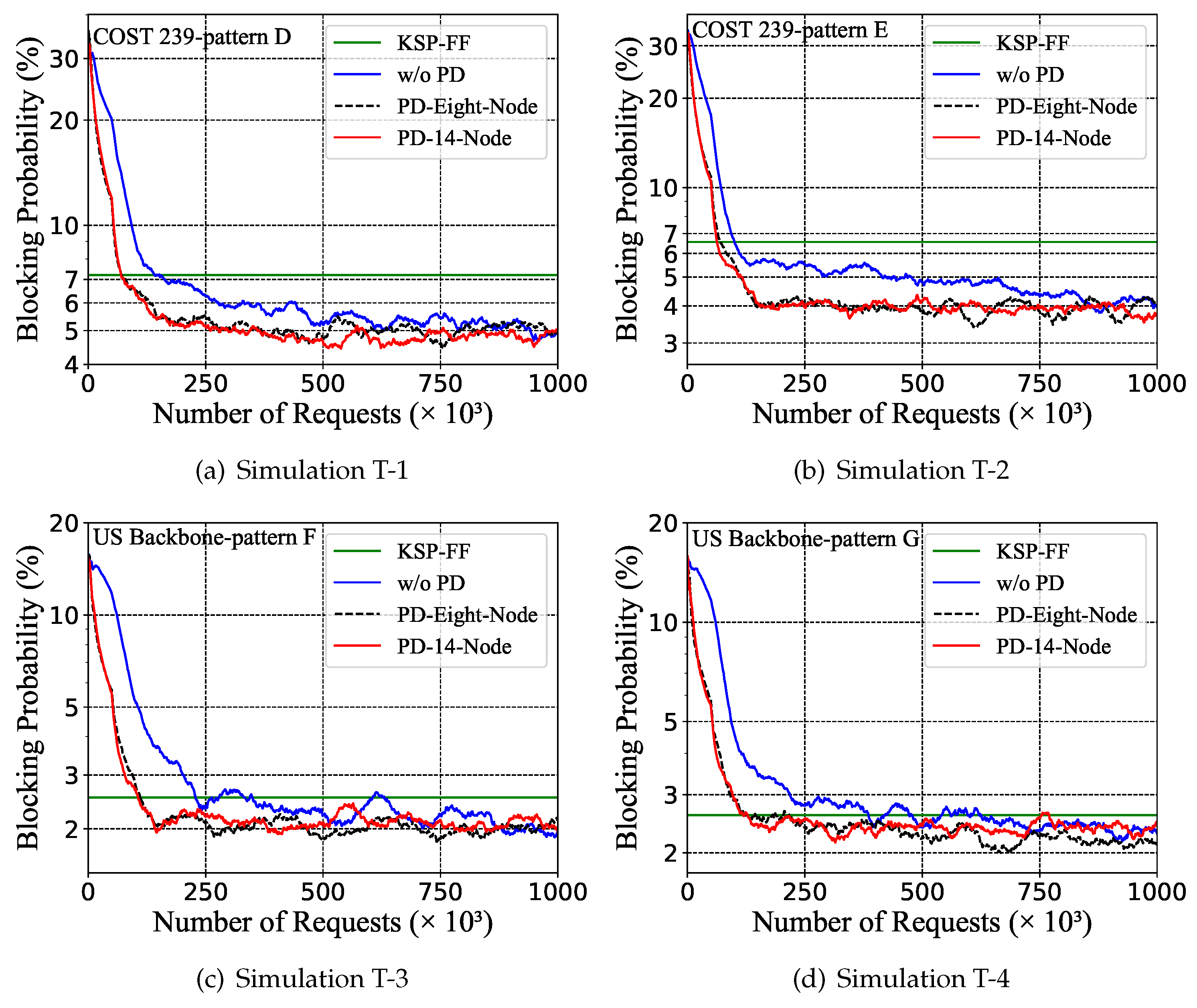
5.2. Policy Distillation for Different Traffic Patterns
- Pattern A: non-uniform; ; .
- Pattern B: non-uniform; ; exist when .
- Pattern C: non-uniform; exist ; exist when .
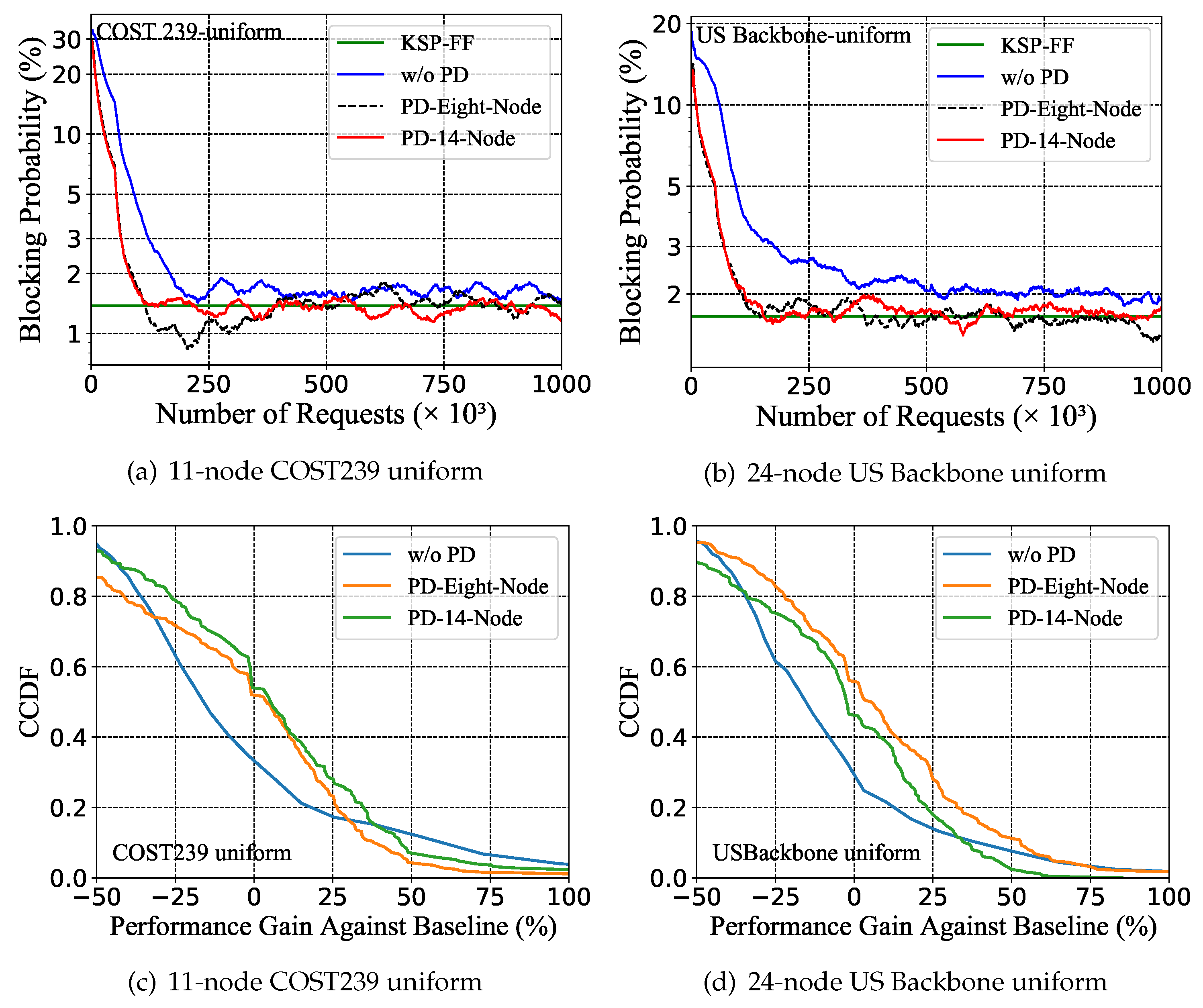
5.3. Policy Distillation for Different Topologies
5.4. Policy Distillation for Different Traffic Patterns and Topologies
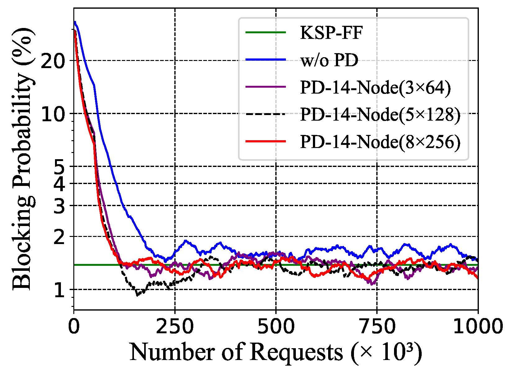
5.5. Policy Distillation with Different Neural Network Size of the Teacher Model
6. Conclusions
Author Contributions
Funding
Institutional Review Board Statement
Informed Consent Statement
Data Availability Statement
Acknowledgments
Conflicts of Interest
References
- Cisco Visual Networking Index: Forecast and Trends, 2017–2022. Available online: https://www.cisco.com/c/en_in/index.html (accessed on 1 November 2018).
- Jinno, M.; Takara, H.; Kozicki, B.; Tsukishima, Y.; Sone, Y.; Matsuoka, S. Spectrum-efficient and scalable elastic optical path network: Architecture, benefits, and enabling technologies. IEEE Commun. Mag. 2009, 47, 66–73. [Google Scholar] [CrossRef]
- Gerstel, O.; Jinno, M.; Lord, A.; Yoo, S.B. Elastic optical networking: A new dawn for the optical layer? IEEE Commun. Mag. 2012, 50, s12–s20. [Google Scholar] [CrossRef]
- Zang, H.; Jue, J.P.; Mukherjee, B. A review of routing and wavelength assignment approaches for wavelength-routed optical WDM networks. Opt. Netw. Mag. 2000, 1, 47–60. [Google Scholar]
- Dinarte, H.A.; Correia, B.V.; Chaves, D.A.; Almeida, R.C. Routing and spectrum assignment: A metaheuristic for hybrid ordering selection in elastic optical networks. Comput. Netw. 2021, 197, 108287. [Google Scholar] [CrossRef]
- Zhang, G.; De Leenheer, M.; Morea, A.; Mukherjee, B. A survey on OFDM-based elastic core optical networking. IEEE Commun. Surv. Tutor. 2012, 15, 65–87. [Google Scholar] [CrossRef]
- Halder, J.; Acharya, T.; Chatterjee, M.; Bhattacharya, U. E-S-RSM-RSA: A novel energy and spectrum efficient regenerator aware multipath based survivable RSA in offline EON. IEEE Trans. Green Commun. Netw. 2021, 5, 1451–1466. [Google Scholar] [CrossRef]
- Halder, J.; Acharya, T.; Bhattacharya, U. On crosstalk aware energy and spectrum efficient survivable RSCA scheme in offline SDM-EON. J. Netw. Syst. Manag. 2022, 30, 6. [Google Scholar] [CrossRef]
- Jia, W.B.; Xu, Z.Q.; Ding, Z.; Wang, K. An efficient routing and spectrum assignment algorithm using prediction for elastic optical networks. In Proceedings of the 2016 International Conference on Information System and Artificial Intelligence (ISAI), Hong Kong, China, 24–26 June 2016; pp. 89–93. [Google Scholar]
- Cavalcante, M.; Pereira, H.; Chaves, D.; Almeida, R. Optimizing the cost function of power series routing algorithm for transparent elastic optical networks. Opt. Switch. Netw. 2018, 29, 57–64. [Google Scholar] [CrossRef]
- Harai, H.; Murata, M.; Miyahara, H. Performance of alternate routing methods in all-optical switching networks. In Proceedings of the International Conference on Computer Communications (INFOCOM), Hong Kong, China, 24–26 June 1997; Volume 2, pp. 516–524. [Google Scholar]
- Ramamurthy, R.; Mukherjee, B. Fixed-alternate routing and wavelength conversion in wavelength-routed optical networks. IEEE/ACM Trans. Netw. 2002, 10, 351–367. [Google Scholar] [CrossRef]
- Rosa, A.; Cavdar, C.; Carvalho, S.; Costa, J.; Wosinska, L. Spectrum allocation policy modeling for elastic optical networks. In High Capacity Optical Networks and Emerging/Enabling Technologies (HONET); IEEE: Piscataway, NJ, USA; New York, NY, USA, 2012; pp. 242–246. [Google Scholar]
- Chen, X.; Li, B.; Proietti, R.; Lu, H.; Zhu, Z.; Yoo, S.B. DeepRMSA: A deep reinforcement learning framework for routing, modulation and spectrum assignment in elastic optical networks. J. Light. Technol. 2019, 37, 4155–4163. [Google Scholar] [CrossRef]
- Huang, Y.C.; Zhang, J.; Yu, S. Self-learning routing for optical networks. In Lecture Notes in Computer Science; Springer: Berlin/Heidelberg, Germany, 2020; pp. 467–478. [Google Scholar]
- Zhao, Z.; Zhao, Y.; Li, Y.; Wang, F.; Li, X.; Han, D.; Zhang, J. Service restoration in multi-modal optical transport networks with reinforcement learning. Opt. Express 2021, 29, 3825–3840. [Google Scholar] [CrossRef] [PubMed]
- Zhao, Y.; Yan, B.; Liu, D.; He, Y.; Wang, D.; Zhang, J. SOON: Self-optimizing optical networks with machine learning. Opt. Express 2018, 26, 28713–28726. [Google Scholar] [CrossRef]
- Xu, L.; Huang, Y.C.; Xue, Y.; Hu, X. Spectrum continuity and contiguity aware state representation for deep reinforcement learning-based routing of EONs. In Proceedings of the IEEE Optoelectronics Global Conference (OGC), Shenzhen, China, 15–18 September 2021; pp. 73–76. [Google Scholar]
- Tang, B.; Chen, J.; Huang, Y.C.; Xue, Y.; Zhou, W. Optical network routing by deep reinforcement learning and knowledge distillation. In Proceedings of the Asia Communications and Photonics Conference (ACP), Shanghai, China, 24–27 October 2021; pp. 1–3. [Google Scholar]
- Chen, X.; Proietti, R.; Liu, C.Y.; Yoo, S.B. A multi-task-learning-based transfer deep reinforcement learning design for autonomic optical networks. IEEE J. Sel. Areas Commun. 2021, 39, 2878–2889. [Google Scholar] [CrossRef]
- Rusu, A.A.; Colmenarejo, S.G.; Gulcehre, C.; Desjardins, G.; Kirkpatrick, J.; Pascanu, R.; Mnih, V.; Kavukcuoglu, K.; Hadsell, R. Policy distillation. In Proceedings of the International Conference on Learning Representations (ICLR), San Juan, Puerto Rico, 2–4 May 2016. [Google Scholar]
- Gou, J.; Yu, B.; Maybank, S.; Tao, D. Knowledge distillation: A survey. Int. J. Comput. Vision. 2021, 129, 1789–1819. [Google Scholar] [CrossRef]
- Chen, X.; Guo, J.; Zhu, Z.; Proietti, R.; Castro, A.; Yoo, S.B. Deep-RMSA: A deep-reinforcement-learning routing, modulation and spectrum assignment agent for elastic optical networks. In Proceedings of the Optical Fiber Communications Conference and Exposition (OFC), San Diego, CA, USA, 11–15 March 2018; pp. 1–3. [Google Scholar]
- Yan, B.; Zhao, Y.; Li, Y.; Yu, X.; Zhang, J.; Wang, Y.; Yan, L.; Rahman, S. Actor-critic-based resource allocation for multi-modal optical networks. In Proceedings of the IEEE Globecom Workshops (GC Wkshps), Abu Dhabi, United Arab Emirates, 9–13 December 2018; pp. 1–6. [Google Scholar]
- Suárez-Varela, J.; Mestres, A.; Yu, J.; Kuang, L.; Feng, H.; Cabellos-Aparicio, A.; Barlet-Ros, P. Routing in optical transport networks with deep reinforcement learning. J. Opt. Commun. Netw. 2019, 11, 547–558. [Google Scholar] [CrossRef]
- Pujol-Perich, D.; Suárez-Varela, J.; Ferriol, M.; Xiao, S.; Wu, B.; Cabellos-Aparicio, A.; Barlet-Ros, P. IGNNITION: Bridging the gap between graph neural networks and networking systems. IEEE Netw. 2021, 35, 171–177. [Google Scholar] [CrossRef]
- Koch, R.; Kühl, S.; Morais, R.M.; Spinnler, B.; Schairer, W.; Sommernkorn-Krombholz, B.; Pachnicke, S. Reinforcement learning for generalized parameter optimization in elastic optical networks. J. Light. Technol. 2022, 40, 567–574. [Google Scholar] [CrossRef]
- Zhao, Z.; Zhao, Y.; Ma, H.; Li, Y.; Rahman, S.; Han, D.; Zhang, H.; Zhang, J. Cost-efficient routing, modulation, wavelength and port assignment using reinforcement learning in optical transport networks. Opt. Fiber Technol. 2021, 64, 102571. [Google Scholar] [CrossRef]
- Li, B.; Zhu, Z. DeepCoop: Leveraging cooperative DRL agents to achieve scalable network automation for multi-domain SD-EONs. In Proceedings of the Optical Fiber Communication Conference (OFC), San Diego, CA, USA, 8–12 March 2020; p. Th2A-29. [Google Scholar]
- Yao, Q.; Yang, H.; Yu, A.; Zhang, J. Transductive transfer learning-based spectrum optimization for resource reservation in seven-core elastic optical networks. J. Light. Technol. 2019, 37, 4164–4172. [Google Scholar] [CrossRef]
- Liu, C.Y.; Chen, X.; Proietti, R.; Yoo, S.B. Evol-TL: Evolutionary transfer learning for QoT estimation in multi-domain networks. In Proceedings of the Optical Fiber Communications Conference and Exhibition (OFC), San Diego, CA, USA, 8–12 March 2020; pp. 1–3. [Google Scholar]
- Mnih, V.; Badia, A.P.; Mirza, M.; Graves, A.; Lillicrap, T.; Harley, T.; Silver, D.; Kavukcuoglu, K. Asynchronous methods for deep reinforcement learning. In Proceedings of the International Conference on Machine Learning (ICML), New York, NY, USA, 19–24 June 2016; pp. 1928–1937. [Google Scholar]
- Konda, V.R.; Tsitsiklis, J.N. Actor-critic algorithms. In Proceedings of the Advances in Neural Information Processing Systems (NeurIPS), Denver, CO, USA; 2000; pp. 1008–1014. [Google Scholar]
- Kozicki, B.; Takara, H.; Sone, Y.; Watanabe, A.; Jinno, M. Distance-adaptive spectrum allocation in elastic optical path network (SLICE) with bit per symbol adjustment. In Proceedings of the Optical Fiber Communications Conference and Exhibition (OFC), San Diego, CA, USA, 8–12 March 2020; pp. 1–3. [Google Scholar]
- Zhu, Z.; Lu, W.; Zhang, L.; Ansari, N. Dynamic service provisioning in elastic optical networks with hybrid single-/multi-path routing. J. Light. Technol. 2012, 31, 15–22. [Google Scholar] [CrossRef]
- Jinno, M.; Kozicki, B.; Takara, H.; Watanabe, A.; Sone, Y.; Tanaka, T.; Hirano, A. Distance-adaptive spectrum resource allocation in spectrum-sliced elastic optical path network. IEEE Commun. Mag. 2010, 48, 138–145. [Google Scholar] [CrossRef]
- Tang, B.; Huang, Y.-C.; Xue, Y.; Zhou, W. Heuristic reward design for deep reinforcement learning-based routing, modulation and spectrum assignment of elastic optical networks. IEEE Commun. Lett. 2022. [Google Scholar] [CrossRef]


| Modulation Format | Transmission Reach | |
|---|---|---|
| 1 | BPSK | 5000 km |
| 2 | QPSK | 2500 km |
| 3 | 8-QAM | 1250 km |
| 4 | 16-QAM | 625 km |
| Notation | Meaning | Value | |
|---|---|---|---|
| DRL Environment (i.e., EONs) | Number of frequency slots per link | 100 | |
| B | Bandwidth requirement | Gb/s | |
| K | Number of candidate paths | 5 | |
| Bandwidth of a spectrum slot | GHz | ||
| DRL agent | L | Number of hidden layers (teacher model/student model) | |
| H | Number of neurons for each hidden layer (teacher model/student model) | ||
| DRL training | Discount rate | ||
| Learning rate | |||
| Entropy regularization coefficient | |||
| N | Mini-batch size | 200 | |
| M | Number of traffic requests for distillation | 100,000 | |
| Temperature | 5 | ||
| Final explore rate | 0.05 |
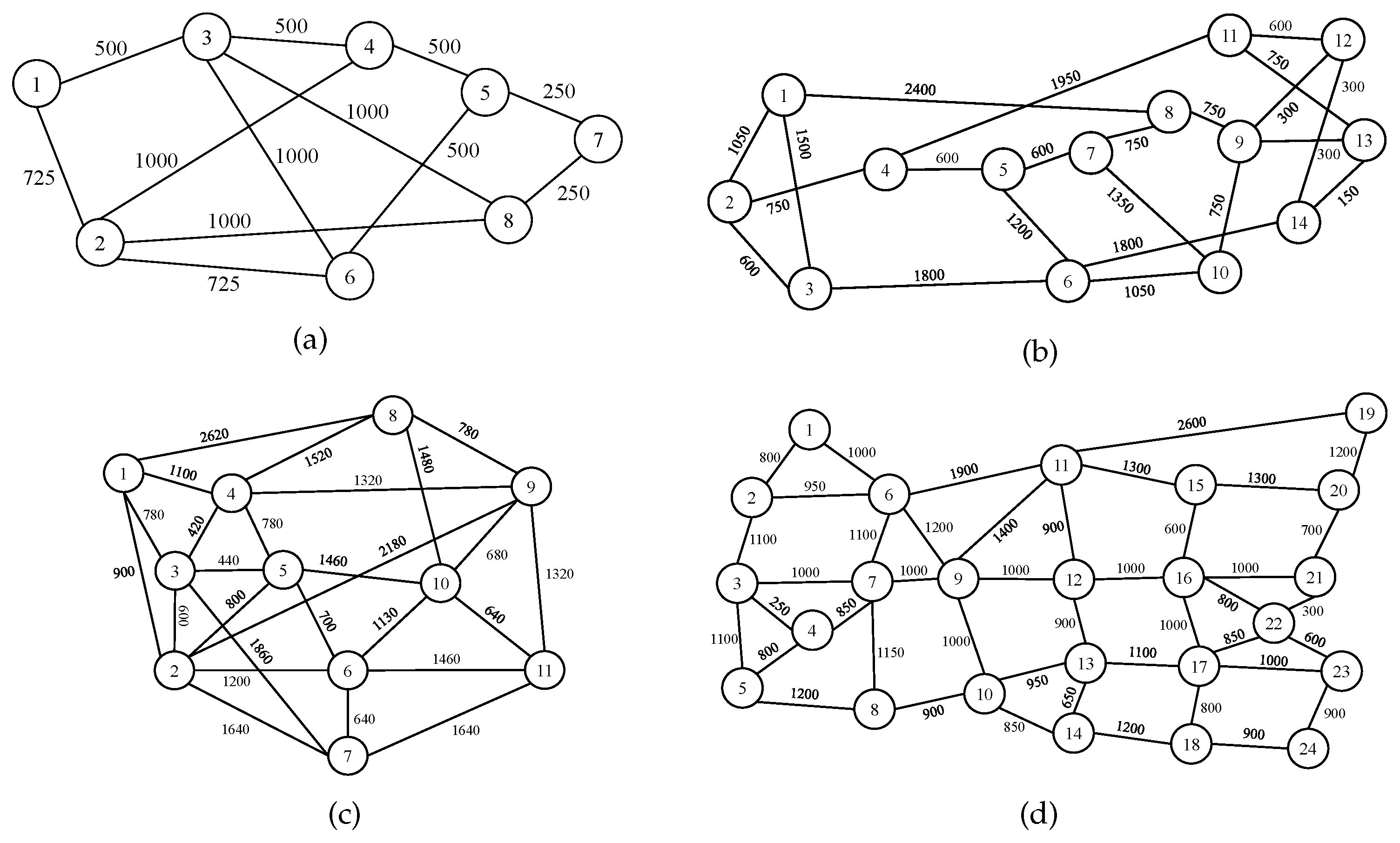
| Topology | Traffic Pattern | Load | |
|---|---|---|---|
| Teacher model | 14-node NSFNET | uniform | |
| Student model | 14-node NSFNET | pattern A | |
| 14-node NSFNET | pattern B | ||
| 14-node NSFNET | pattern C |
| Topology | Traffic Pattern | Load | |
|---|---|---|---|
| Teacher model | 8-node | uniform | |
| 14-node NSFNET | uniform | ||
| Student model | 11-node COST 239 | uniform | |
| 24-node US Backbone | uniform |
| Student Model | ||
|---|---|---|
| Simulation T-1 | Topology | 11-node COST239 |
| Traffic pattern | pattern D (non-uniform; ; ) | |
| Simulation T-2 | Topology | 11-node COST239 |
| Traffic pattern | pattern E (non-uniform; ; exist when ) | |
| Simulation T-3 | Topology | 24-node US Backbone |
| Traffic pattern | pattern F (non-uniform; ; ) | |
| Simulation T-4 | Topology | 24-node US Backbone |
| Traffic pattern | pattern G (non-uniform; ; exist when ) |
| Topology | Traffic Pattern | Load | |
|---|---|---|---|
| Teacher model | 8-node | uniform | |
| 14-node NSFNET | uniform | ||
| Student model | 11-node COST 239 | pattern D | |
| 11-node COST 239 | pattern E | ||
| 24-node US Backbone | pattern F | ||
| 24-node US Backbone | pattern G |
| “PD-Eight-Node” | “PD-14-Node” | “w/o PD” | |
|---|---|---|---|
| Simulation T-1 | 1963 | 1956 | 2863 |
| Simulation T-2 | 1939 | 1895 | 2258 |
| Simulation T-3 | 3131 | 2868 | 7277 |
| Simulation T-4 | 3743 | 3373 | 9427 |
Publisher’s Note: MDPI stays neutral with regard to jurisdictional claims in published maps and institutional affiliations. |
© 2022 by the authors. Licensee MDPI, Basel, Switzerland. This article is an open access article distributed under the terms and conditions of the Creative Commons Attribution (CC BY) license (https://creativecommons.org/licenses/by/4.0/).
Share and Cite
Tang, B.; Huang, Y.-C.; Xue, Y.; Zhou, W. Deep Reinforcement Learning-Based RMSA Policy Distillation for Elastic Optical Networks. Mathematics 2022, 10, 3293. https://doi.org/10.3390/math10183293
Tang B, Huang Y-C, Xue Y, Zhou W. Deep Reinforcement Learning-Based RMSA Policy Distillation for Elastic Optical Networks. Mathematics. 2022; 10(18):3293. https://doi.org/10.3390/math10183293
Chicago/Turabian StyleTang, Bixia, Yue-Cai Huang, Yun Xue, and Weixing Zhou. 2022. "Deep Reinforcement Learning-Based RMSA Policy Distillation for Elastic Optical Networks" Mathematics 10, no. 18: 3293. https://doi.org/10.3390/math10183293
APA StyleTang, B., Huang, Y.-C., Xue, Y., & Zhou, W. (2022). Deep Reinforcement Learning-Based RMSA Policy Distillation for Elastic Optical Networks. Mathematics, 10(18), 3293. https://doi.org/10.3390/math10183293