Anomaly Detection Algorithm Based on Broad Learning System and Support Vector Domain Description

Abstract

Deep neural network-based autoencoders can effectively extract high-level abstract features with outstanding generalization performance but suffer from sparsity of extracted features, insufficient robustness, greedy training of each layer, and a lack of global optimization. In this study, the broad learning system (BLS) is improved to obtain a new model for data reconstruction. Support Vector Domain Description (SVDD) is one of the best-known one-class-classification methods used to solve problems where the proportion of sample categories of data is extremely unbalanced. The SVDD is sensitive to penalty parameters C, which represents the trade-off between sphere volume and the number of target data outside the sphere. The training process only considers normal samples, which leads to a low recall rate and weak generalization performance. To address these issues, we propose a BLS-based weighted SVDD algorithm (BLSW_SVDD), which introduces reconstruction error weights and a small number of anomalous samples when training the SVDD model, thus improving the robustness of the model. To evaluate the performance of BLSW_SVDD model, comparison experiments were conducted on the UCI dataset, and the experimental results showed that in terms of accuracy and F1 values, the algorithm has better performance advantages than the traditional and improved SVDD algorithms.

1. Introduction

With the rapid development of Internet technology, the volume and type of data are exploding; in the data acquisition process, we generally encounter data that are quite distinct from the entire dataset, and this can affect the analysis and analysis-based decision making. Traditional anomaly detection algorithms need to acquire and label many normal and abnormal samples. However, in practical problems, abnormal labels may not be available, such as in the case of aircraft failure and earthquake disasters, which are difficult to obtain. One-class-classification algorithms can effectively resolve such situations. The support vector domain description (SVDD) classifier, a typical one-class classifier, was first proposed by Tax and Duin [1,2]. The basic idea of this algorithm is to first map the data samples from the original input data space to a high-dimensional feature space. Further, it finds the smallest hypersphere in the high-dimensional feature space that contains as much target data as possible while rejecting most anomalous data. It can rely on only a small number of support vectors (SVs) on the sphere to obtain a very flexible and accurate description of the domain. SVDD is currently applied to several fields such as industrial anomaly detection [3] and disease detection [4].

Despite the usefulness of the SVDD classifiers, problems such as difficulties in selecting penalty parameters remain. Some researchers have successively made improvements to SVDD. The data domain description is susceptible to the penalty parameter C’ choice, which significantly effects on the boundary description of the domain but is difficult to estimate in practice. To solve this problem and find better outlier detection algorithms, researchers have proposed improved SVDD algorithms. Lee et al. [5,6] proposed the density-induced SVDD algorithm (DI-SVDD) in 2007, which introduced a weighting based on each training data point’s spatial distribution of density. In 2013, Wang and Lai [7] proposed the position regularized support vector data domain description algorithm (P_SVDD) which adaptively regularizes the complexity of the sphere by assigning a position-based weight to each training data point based on the Euclidean distance between each training data point and mean points in the mapped feature space. Cha et al. [8] proposed the density weighted support vector domain description algorithm (DW_SVDD), which introduced the concept of density weights to search for the optimal domain description by calculating the relative density of each training data point according to the data distribution in the original space and replacing the penalty parameters of the corresponding slack variables. Tao et al. [9] assigned corresponding weights to each training data according to the distribution of spatial location and density of each training data point to obtain a spherical data description of the training data, and a new weighted SVDD anomaly detection algorithm (AW_SVDD) was proposed. The results and performance of SVDD are significantly affected when the target data samples are irregularly distributed and have widely different density distributions. To address this problem, an anomaly detection algorithm (KM_SVDD) based on SVDD and K-means clustering algorithm was proposed by Xu et al. [10]. Wu et al. [11] combined the affinity propagation (AP) clustering algorithm and SVDD and proposed an adaptive SVDD algorithm (SA_SVDD). To map the data point into a compact domain description, more suitable for being surrounded by hyperspheres, Sohrab et al. [12] proposed a subspace support vector data description algorithm (SSVDD), which maps the training data points to a subspace optimized for a target class by non-linear mapping. Further, it determines the best hypersphere in the feature space that encloses the target class. Ruff, L. et al. [13] proposed Deep Support Vector Data Description (Deep SVDD) replacing the mapping function in traditional SVDD by training a neural network such that the volume of the hypersphere containing as many target class samples as possible is minimized. Hojjati, H. et al. [14] proposed an anomaly detection algorithm (DASVDD)-based Deep Autoencoder and SVDD, which learns the basic distribution of target class by minimizing the combined anomaly score of the autoencoder’s reconstruction error and the distance from the sample to the center of the closed hypersphere in training. Including the reconstruction error in the anomaly score ensures that DASVDD does not suffer from the common hypersphere runout problem.

Compared with the traditional SVDD, some improved SVDD algorithms described above are effective in terms of performance. However, the calculation of weights depends on the distributions of spatial location and density feature of data points in the feature space. It is ineffective for training sets with insignificant spatial location and density distributions. To solve this challenge, we propose a novel anomaly detection algorithm (BLSW_SVDD) based on BLS and SVDD, which first uses the normal training dataset to improve the BLS network, trains to construct a data reconstruction model, and then assigns a weight based on reconstruction error to each training data point when training the SVDD model. The value of reconstruction error reflects the likelihood of each data point becoming an outlier. Using normal samples alone to train SVDD is vulnerable to the attack of anomalous samples, which degrades the efficiency and performance of the SVDD model [15]. Therefore, the BLSW_SVDD model proposed in this paper adds a small number of anomalous samples to the training samples. To evaluate the performance of the BLSW_SVDD algorithm, experiments were conducted on datasets from the UCI repository. The experimental results demonstrate that the BLSW_SVDD algorithm outperforms traditional SVDD and improved SVDD algorithms in terms of accuracy and F1 value. Its performance in the data domain description was improved. It overcomes the difficult selection of penalty parameters by traditional SVDD has a better generalization performance.

The rest of the paper is organized as follows. In Section 2, we introduce the brief related works for BLS and SVDD. In Section 3, we mainly discuss more details about the BLSW_SVDD model, including the model inferring process and structure. In Section 4, we design the experiments to evaluate the performance of BLSW_SVDD model and analyze the experimental results from different perspectives. Finally, we draw conclusions in Section 5.

2. Related Work

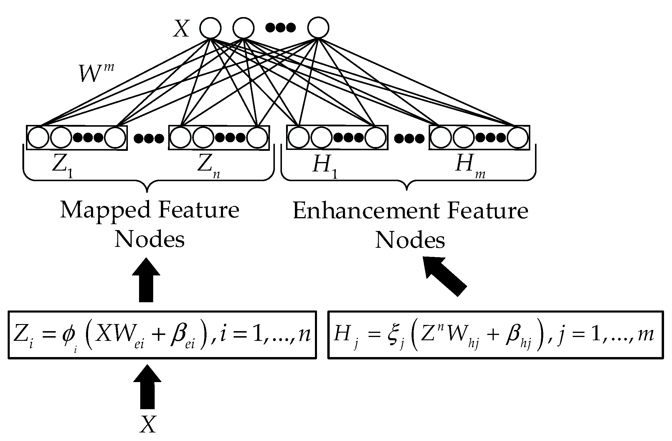
2.1. Overview of the Broad Learning System

Deep structured neural networks, which can effectively extract high-level abstract features and have outstanding generalization performance, have been applied in many areas with extraordinary achievements, especially in large-scale data processing [16,17]. The more famous deep structured networks are deep belief networks (DBNs) [18,19], deep Boltzmann machines (DBMs) [20], and convolutional neural networks (CNNs) [21,22]. Although deep structured networks are so powerful, they require a large number of iterations for training due to a large number of hyperparameters in their complex multi-layer stacked networks, which consume a lot of computational resources and time. At the same time, training methods based on backpropagation and gradient descent are prone to suffering from slow convergence and being trapped in local optimal. In the face of newly added samples involving the whole network, it is difficult to quickly update its deep structure parameters and to analyze the deep structure at a theoretical level. Therefore, most of the work has focused on stacking more layers in the deep structure network or continuously adjusting the network structure parameters to obtain better performance. Pao et al. [23,24] proposed a random vector function linked neural network (RVFLNN), which uses the original input data layer and enhancement feature node layer serve as the total input layer to the network. Then, the pseudo-inverse method can quickly find the weights, effectively solving the drawback of requiring a large amount of training time in deep structured networks. RVFLNN has a powerful function approximation generalization capability [25], fast learning properties, and continuous generalization approximation capability. Currently, it is widely used to solve regression and classification problems due to the approximate generalization capability.

As the accuracy of RVFLNN model was insufficient to support the data’s modeling requirements as the data volume continued to increase, Chen and Liu proposed the broad learning system (BLS) based on the RVFLNN network at the 32nd Annual Young Academics Conference [26] in 2017. In a paper published in 2018 [27], Chen and Lui carried out further research on BLS, refining the theoretical knowledge of BLS. Compared with RVFLNN, the BLS network adds a sparse coding algorithm and a feature node layer in the hidden layer, which performs the primary feature extraction on the original input data. In addition, the BLS incorporates a dynamic stepwise update algorithm, which can quickly optimize the model for newly added hidden layer nodes or newly added samples without re-modelling, thus saving much time and being highly efficient. Many research scholars have conducted studies on BLS. Chu, F. et al. [28] proposed a weighted BLS-based model (BBLS) to solve the problem of data noise and outliers in industrial processes. To improve the robustness of BLS, Zheng, Y. et al. [29] proposed to train the output weights using the maximum correlation entropy criterion (MCC) to obtain a broad learning system model based on correlation entropy (C-BLS). Zhang, L. et al. [30] proposed four variants of BLS networks and incremental implementations based on the structure of deep neural networks. Huang, P. et al. [31] proposed a bidirectional broad learning system (B_BLS) that minimizes the number of hidden layer nodes without compromising the performance of BLS. In the paper [32], Lili Xu proposed that they assembled some of the best performing activation functions, obtaining better performance than the corresponding individual activation functions in the standard BLS. Existing BLS models are not directly applicable for large-scale multi-label learning due to the large and complex label space. Therefore, a novel multi-label classifier based on BLS (called BLS-MLL) is proposed by Pu, X. et al. [33]. Considering that in many practical applications, training data are sequentially generated, an online semi-supervised broad learning system (OSSBLS) is proposed for fault diagnosis in these cases by Huang, J. et al. [34].

So far, it has been applied to many fields, such as drift compensation [35], image classification [36], and collaborative localization [37].

2.2. Broad Learning System (BLS)

The broad learning system provides a simple new algorithmic structure that does not rely on deep structural layers. As shown in Figure 1, the basic architecture of the BLS consists of an input layer, a hidden layer including mapped feature nodes and enhancement feature nodes, and an output layer.

The input data of the BLS are assumed to be $X\in R^{N\times D}$, $N$ and $D$ denote the number of data samples and the feature dimension of the samples, respectively, and the output data are denoted by $Y\in R^{N\times C}$, where $N$ denotes the number of data samples and $C$ represents the number of categories of the samples. Figure 1 shows that the BLS network has $n$ groups of mapped feature nodes and $m$ groups of enhancement feature nodes. Each group of mapped feature nodes has $p$ feature nodes, and the $i$-th group of mapped feature nodes is generated by random mapping, as shown in Equation (1).

$$Z_i={\varphi }_i\left(X{W}_{ei}+{\beta }_{ei}\right),$$

(1)

where $W_{ei}$ and ${\beta }_{ei}$ are the weights and biases of the appropriate randomly generated dimensions and ${\varphi }_i(·)$ is the mapping function. Since the sparse feature model [38] can be effective in learning and obtaining good feature representations and useful feature information from the data samples, the classical sparse autoencoder [39] was utilized in generating the mapping feature nodes layer to extract the sparse feature points in the input data matrix, with a slight fine-tuning of $W_{ei}$ and ${\beta }_{ei}$.

These randomly generated mapped feature nodes are then stitched together, denoted as $Z^n=\left[Z_1,Z_2\dots ,Z_n\right]$. The BLS will use these mapped feature nodes to form the $Z^n$ and extend the enhancement feature nodes layer by a non-linear activation function ${\xi }_j(·)$. Each set of enhancement feature nodes has of $q$ nodes, and the$j$-th enhancement feature node is denoted as Equation (2).

$$H_j={\xi }_j\left(Z^n{W}_{hj}+{\beta }_{hj}\right),$$

(2)

where $W_{hj}$ and ${\beta }_{hj}$ are the weights and biases of the appropriate randomly generated dimensions. Similar to the previous step, the $m$ enhancement feature nodes are joined horizontally, which can be expressed as $H^m=\left[H_1,H_2\dots ,H_m\right]$.

The output feature matrix $A$ of the BLS, denoted by $A=[Z^n\mid H^m]\in R^{N\times (np+mq)}$, can be obtained by horizontally concatenating the mapped features nodes $Z^n$ and the enhancement feature nodes $H^m$ into a matrix. The final output layer representation of the broad learning system is obtained by calculating the multiplication of the feature matrix and connection weights, so that the output $Y$ of the BLS can be expressed as:

$$Y=A{W}^m,$$

(3)

where $W^m$ denotes the connection weights of the BLS network from the hidden layer to the output layer. The pseudo-inverse algorithm can easily obtain the weights of the output layer in a randomized weight-plane neural network. Thus, the weights of the output layer $W^m$ can be quickly calculated using $W^m=A^{+}Y$, where $A^{+}$ is the pseudo-inverse matrix of the BLS feature matrix $A$. However, owing to the sheer volume and dimensionality of the dataset, it is too expensive to utilize standard methods such as orthogonal projection, iteration, and singular value decomposition to compute the generalized inverse. By introducing parametric regularization, the problem of solving the pseudo-inverse of a matrix can be expressed as the following optimization problem:

$$\arg \underset{w}{\min }{\Vert A{W}^m-Y\Vert }^2+\lambda {\Vert W^m\Vert }^2,$$

(4)

regularization constraint term λ is added to the original least-squares estimate to enable the original generalized inverse to determine the pseudo-inverse under pathological conditions. Thus, $W^m$ can be calculated as follows:

$$W^m={\left(\lambda I+A{A}^T\right)}^{-1}{A}^{T}Y,$$

(5)

then, $A^{+}=\underset{\lambda \to 0}{\lim }{\left(\lambda I+A{A}^T\right)}^{-1}{A}^T$, where $I$ is the unit matrix.

2.3. Support Vector Domain Description (SVDD)

Given a dataset $X=\{x_i\in R^d|i=1,\dots ,n\}$, the goal of the SVDD is to construct a minimal volume hypersphere with center $\mu$ and radius $R$ containing all or most normal samples, the structure of which is illustrated in Figure 2.

We introduce the slack variable ${\xi }_i$ to allow some of the samples to be erroneously classified and be outside the hyperspheres. The objective of the SVDD algorithm is shown in Equation (6).

$$\begin{array}{l}\min F\left(R,\mu ,{\xi }_i\right)=R^2+C{\displaystyle \sum _{i=1}^n{\xi }_i}\\ s.t. {\Vert \varphi \left(x_i\right)-\mu \Vert }^2\le R^2+{\xi }_i,{\xi }_i\ge 0,\forall i=1,\dots ,n\end{array}$$

(6)

where C is the penalty parameter that controls the degree of punishment for samples that do not satisfy the constraint, and $\varphi (·)$ is a non-linear transformation from mapping the input data from the input space to a high-dimensional feature space. By introducing Lagrange multipliers ${\alpha }_i\ge 0$ and ${\beta }_i\ge 0$, the objective function of Equation (6) can be transformed into the optimization problem in Equation (7) as follows:

$$\begin{array}{l}L\left(R,\mu ,{\xi }_i,{\alpha }_i,{\beta }_i\right)=R^2+C{\displaystyle \sum _{i=1}^n{\xi }_i}\\ -{\displaystyle \sum _{i=1}^n{\alpha }_i}\left(R^2+{\xi }_i-{\Vert \varphi \left(x_i\right)-\mu \Vert }^2\right)-{\displaystyle \sum _{i=1}^n{\beta }_i}{\xi }_i\end{array}$$

(7)

The partial derivatives of the variables $R,\mu ,{\xi }_i$ in Equation (7) are then calculated, and the values of these partial derivatives are zero, which can be expressed as shown in Equations (8)–(10), respectively:

$$\frac{\partial L}{\partial R}=0\to {\displaystyle \sum _{i=1}^n{\alpha }_i}=1,$$

(8)

$$\frac{\partial L}{\partial \mu }=0\to \mu ={\displaystyle \sum _{i=1}^n{\alpha }_i}\varphi \left(x_i\right),$$

(9)

$$\frac{\partial L}{\partial {\xi }_i}=0\to C-{\alpha }_i-{\beta }_i=0.$$

(10)

Replacing the inner product $\left(x_i·x_i\right)$ with the kernel function $K\left(x_i,x_i\right)$ gives the dual form, expressed in Equation (11).

$$\begin{array}{l}\max {\displaystyle \sum _{i=1}^n{\alpha }_i}K\left(x_i,x_i\right)-{\displaystyle \sum _{i=1}^n{\displaystyle \sum _{j=1}^n{\alpha }_i{\alpha }_j}}K\left(x_i,x_j\right)\\ s.t. 0\le {\alpha }_i\le C\\ {\displaystyle \sum _{i=1}^n{\alpha }_i}=1, \forall i=1,\dots ,n\end{array}$$

(11)

Equation (9) indicates that the center of the hypersphere is a linear combination of data objects, and the weight factor ${\alpha }_i$ is obtained by optimizing Equation (11). $K\left(x_i,x_j\right)$ is a kernel function that satisfies Mercer’s theorem and can map the data to a certain feature space. This study uses a Gaussian kernel function expressed in Equation (12), where $q$ is the kernel parameter.

$$K\left(x_i,x_j\right)=\exp \left(-q{\Vert x_i-x_j\Vert }^2\right).$$

(12)

Data points can be classified into three types based on the value of the Lagrange multiplier.

(1)

Interior points (IP): ${\alpha }_i=0$, the corresponding sample $\varphi \left(x_i\right)$ lies within the hypersphere.

(2)

Support vectors (SV): $0\le {\alpha }_i\le C$, the corresponding sample $\varphi \left(x_i\right)$ lies on the boundary of the hypersphere.

(3)

Boundary support vector (BSV): ${\alpha }_i=C$, the corresponding sample $\varphi \left(x_i\right)$ lies outside the hypersphere.

The sphere radius $R$ can be obtained by calculating the distance between the sphere’s center and the support vector (SV). Ideally, all the SVs should have the same radius. However, because of numerical problems, they may be slightly different. A practical strategy is to use their maximum values as radii, which can be expressed using Equation (13).

$$\begin{array}{cc}\hfill R^2& ={\Vert \varphi \left(x_i\right)-\mu \Vert }^2\hfill \\ & =1-2{\displaystyle \sum _{i=1}^n{\alpha }_i}K\left(x_i,x_i\right)+{\displaystyle \sum _{i=1}^n{\displaystyle \sum _{j=1}^n{\alpha }_i{\alpha }_j}}K\left(x_i,x_j\right)\hfill \\ \hfill R& =\max \left\{R\left(x_i\right)|x_i is a SV,0\le {\alpha }_i\le C \right\}\hfill \end{array}$$

(13)

To determine whether a specific sample $Z$ to be tested is inside the hypersphere, the distance from the test data point $Z$ to the center of the sphere must be calculated, and the calculation formula is given by Equation (14).

$$f(Z)=\varphi \left(Z,Z\right)-2{\displaystyle \sum _{i=1}^n{\alpha }_i}K\left(x_i,x_i\right)+{\displaystyle \sum _{i=1}^n{\displaystyle \sum _{j=1}^n{\alpha }_i{\alpha }_j}}K\left(x_i,x_j\right).$$

(14)

If $f(Z)\le R^2$ and the test data point $Z$ is within the hypersphere, it is a normal class sample, and otherwise it is an abnormal class sample.

3. Fundamentals of Anomaly Detection Model Based on BLS and SVDD

3.1. Data Reconstruction Model Based on BLS

An autoencoder based on the deep neural network can effectively extract high-dimensional feature representations of data with outstanding generalization performance. However, it has problems such as the sparsity of extracted features, insufficient robustness, greedy training of each layer, and a lack of global optimization. Therefore, a model for constructing reconstructed data based on BLS networks was proposed, and its structure is shown in Figure 3.

To construct a data reconstruction model using BLS network, we should approximate the output of the output layer to the original input. The traditional BLS network is primarily used for supervised sample classification problems, and the corresponding output is the sample category label vector corresponding to the training samples. The flow of the data reconstruction model is as follows:

(1)

Suppose the original input dataset is $X\in R^{N\times D}$; $N$ and $D$ denote the number and feature dimension of the data samples, respectively. According to Equations (1) and (2), we calculate to get the corresponding mapped feature nodes $Z^n$ and enhancement feature nodes $H^m$, respectively. By connecting the mapped feature nodes and enhancement feature nodes horizontally, we obtain the output feature matrix of the BLS, represented as $A=[Z^n|H^m]$.

(2)

Construct the data reconstruction model. Let $Y=\overline{X}$, and $\overline{X}$ be the data matrix after reconstruction. We can then obtain the output expression as follows:

$$\overline{X}=A{W}^m.$$

(15)

(3)

Similar to the solution method described above, Equation (15) can be expressed as $W^m=A^{+}X$, where $A^{+}$ is the pseudo-inverse matrix of the matrix $A$. Subsequently, by introducing parametric regularization, the problem of solving the pseudo-inverse of a matrix can be expressed as the following optimization problem.

$$\arg \underset{w}{\min }{\Vert A{W}^m-\overline{X}\Vert }^2+\lambda {\Vert W^m\Vert }^2,$$

(16)

Thus, $W^m$ can be calculated as follows:

$$W^m={\left(\lambda I+A{A}^T\right)}^{-1}{A}^T\overline{X}.$$

(17)

In the autoencoder built on BLS, the input data are first mapped to the random feature space and then further mapped to the enhancement feature space. Thus, the more effective feature information of the original input data is obtained before reconstruction, which allows the reconstruction matrix to be trained more accurately. The BLS-based autoencoder utilizes ridge regression to solve the reconstruction matrix, accelerating the reconstruction of the original input data and having good generalization performance. The traditional autoencoder based on deep learning trains the network using a back-propagation algorithm, which incurs considerable time. In contrast, the BLS-based autoencoder has fast learning ability and excellent generalization performance.

3.2. Data Reconstruction Error Weights

The reconstruction error weights are obtained by using normal datasets to train the reconstruction network based on BLS network. Using Equation (15), we can obtain the reconstruction data matrix for normal and abnormal data, then the reconstruction error weight for each data point $w\left(x_i\right)$ can be expressed as follows:

$$w\left(x_i\right)=\frac{1}{{\Vert x_i-{\overline{x}}_i\Vert }^2}.$$

(18)

Then, the compression and reconstruction of the input data can be achieved using the BLS. A well-trained data-reconstruction matrix ensures that the error between the input data point $x_i$ and reconstruction data point ${\overline{x}}_i$ is sufficiently small. When a particular test data point $x_i$ is a normal sample, the error between the input $x_i$ and reconstruction output ${\overline{x}}_i$ is extremely small, the corresponding $w\left(x_i\right)$ is considerable, and the slack variable ${\xi }_i$ is small. As there is a large difference between the normal test sample and the abnormal test sample, and the normal sample is used for training $W^m$, when the test sample point $x_i$ is an abnormal sample, the error between the input $x_i$ and ${\overline{x}}_i$ is large and the corresponding $w\left(x_i\right)$ is extremely small and the larger the slack variable ${\xi }_i$ is, the greater the possibility that the data sample is abnormal.

3.3. Reconstruction Error Weighting-Based SVDD Algorithm

According to the above analysis, each data point should use a different penalty parameter that reflects the confidence level reflecting that each data point is an outlier. The traditional SVDD algorithm uses the same penalty parameter C for all training data points when constructing hyperspherical boundaries. This assumption that the probability of becoming an outlier was the same for each training data point is inaccurate. According to the above analysis, each data point should use a different penalty parameter that reflects the confidence level reflecting that each data point is an outlier. Therefore, this study proposes replacing the penalty parameter C with the reconstructed error value of each training data point to indicate the likelihood that the corresponding data point lies outside the hypersphere. The reconstruction error value of each data point $w\left(x_i\right)$ obtained from Equation (18) is introduced into the SVDD algorithm to obtain the objective function as shown in Equation (19):

$$\begin{array}{l}\min F\left(R,\mu ,{\xi }_i\right)=R^2+{\displaystyle \sum _{i=1}^n w\left(x_i\right){\xi }_i}\\ s.t. {\Vert \varphi \left(x_i\right)-\mu \Vert }^2\le R^2+w\left(x_i\right){\xi }_i,{\xi }_i\ge 0,\forall i=1,\dots ,n\end{array}$$

(19)

By introducing Lagrange multipliers ${\alpha }_i\ge 0$ and ${\beta }_i\ge 0$, the objective function of Equation (19) can be transformed into the following:

$$\begin{array}{l}L\left(R,\mu ,{\xi }_i,{\alpha }_i,{\beta }_i\right)=R^2+w \left(x_i\right) {\displaystyle \sum _{i=1}^n{\xi }_i}\\ -{\displaystyle \sum _{i=1}^n{\alpha }_i}\left(R^2+{\xi }_i-{\Vert \varphi \left(x_i\right)-\mu \Vert }^2\right)-{\displaystyle \sum _{i=1}^n{\beta }_i}{\xi }_i\end{array}$$

(20)

Letting the partial derivative of the objective function L with respect to variables$R,\mu ,{\xi }_i$ be zero, the constraints can be obtained as follows:

$${\displaystyle \sum _{i=1}^n{\alpha }_i}=1, \mu ={\displaystyle \sum _{i=1}^n{\alpha }_i}\varphi \left(x_i\right), {\alpha }_i=w\left(x_i\right)-{\beta }_i.$$

(21)

By eliminating the variables $R,\mu ,{\xi }_i,{\beta }_i$ and replacing the inner product $\left(x_i·x_i\right)$ with the kernel function $K\left(x_i,x_i\right)$, the objective function (20) can be transformed into the Wolfe dual form, as shown in Equation (22):

$$\begin{array}{l}\max {\displaystyle \sum _{i=1}^n{\alpha }_i}K\left(x_i,x_i\right)-{\displaystyle \sum _{i=1}^n{\displaystyle \sum _{j=1}^n{\alpha }_i{\alpha }_j}}K\left(x_i,x_j\right)\\ s.t. 0\le {\alpha }_i\le w\left(x_i\right) \\ {\displaystyle \sum _{i=1}^n{\alpha }_i}=1, \forall i=1,\dots ,n\end{array}$$

(22)

By optimizing Equation (22), we can obtain the value of ${\alpha }_i$ corresponding to each training data point $x_i$. The hypersphere center is obtained by Equation (9). Similarly, the hypersphere radius $R$ can be obtained by Equation (13). To determine whether a test sample $Z$ is within the hypersphere, the distance from the test data point $Z$ to the center of the sphere is first calculated using Equation (14). If $f(Z)\le R^2$, then the test data point $Z$ is a normal class sample within the hypersphere. Otherwise, it is an abnormal sample.

3.4. Framework of the BLSW_SVDD Model

The detailed steps of the BLSW_SVDD model are as follows.

(1)

Training the data-reconstruction model. First, the dataset $X$ is divided into a normal dataset and an abnormal dataset. The normal dataset is utilized for training the reconstruction error weight matrix $W^{\mathrm{m}}$ of the BLS network. Subsequently, the reconstruction data matrix of the normal data and the abnormal data (${\overline{X}}_{normal}$ and ${\overline{X}}_{abnormal}$) can be obtained using Equation (15).

(2)

The reconstruction error weights are calculated. The normal dataset and the abnormal dataset are partitioned with 70% of the data for training the SVDD model and the remaining 30% of the data for testing the SVDD model (i.e., $X_{train}$ and $X_{test}$). Correspondingly, 70% of the normal reconstructed data and 70% of the abnormal reconstructed data are removed to obtain the reconstructed error matrix of the training set ${\overline{X}}_{train}$, and the remaining 30% of the normal reconstructed data and abnormal reconstructed data are used as the reconstructed error matrix of the test set ${\overline{X}}_{test}$. The reconstruction error value of each training data point can be obtained using Equation (18).

(3)

Training the SVDD. The SVDD model is trained by assigning a weight based on the reconstruction error to each training data point in the $X_{train}$ and replacing the penalty parameter $C$ to obtain the center $\mu$ of the minimum hypersphere and the minimum hypersphere radius $R$.

(4)

Testing and anomaly detection. The distance from the data point Z in the test dataset$X_{test}$ to the center of the hypersphere is calculated using Equation (14). If $f(Z)\le R^2$, then the test data point Z is within the hypersphere and is a normal class sample, otherwise, it is an abnormal class sample.

4. Experiment and Analysis

4.1. Experimental Setup and Datasets

To evaluate the performance of the proposed BLSW_SVDD model, we used 12 datasets collected from the UCI repository, described in

Table 1. UCI dataset used in the experiment.

Datasets	Sample Points	Dimensionality	Outliers (%)
Wbc	378	30	21 (5.6%)
Haberman’s survival	306	3	81 (26.4%)
Inosphere	351	34	126 (36%)
Arrhythmia	452	274	66 (15%)
Wdbc	569	30	212 (27.1%)
Breast Wisconsin	683	9	239 (35%)
Glass	214	9	9 (4.2%)
Banknote authentication	1372	4	610 (45%)
Vowels	1456	12	50 (3.4%)
Cardio	1831	21	176 (9.6%)
Pendigits	6870	16	156 (2.27%)
Annthyroid	7200	6	534 (7.42%)

. The choice of parameters has a very significant impact on the performance of the BLSW_SVDD algorithm. The kernel function used in this study was a Gaussian kernel function. The traditional SVDD generally has two parameters that need to be optimized appropriately, the kernel parameter $q$ and the penalty parameter $C$. In this model, because $C$ is replaced with the reconstruction error weight of each training data point, only the kernel parameter $q$ needs to be optimized appropriately. This experiment used a Bayesian parameter optimization algorithm and a 10-fold cross-validation method to optimize $q$ in an optimization range of [2⁻⁶, 2⁶]. The Gaussian model was used as a probabilistic proxy model in the Bayesian parameter optimization algorithm, and the employed collection function was the expectation increment.

In the BLS network, the number of enhancement nodes per group ($N_e$) in was set to 500, the number of mapped feature nodes per group ($N_f$) was 10, the number of groups of mapped feature nodes ($N_{\mathrm{m}}$) was 10, the regularization factor ($\lambda$) was 2⁽⁻³⁰⁾, the nonlinear activation function used was the tansigmoid function, and the kernel parameter coefficient (s) was 0.8.

BLSW_SVDD model is executed by solving a quadratic programming (QP). Therefore, its computational complexity is equal to O(N3). Finally, these experiments have been performed in MATLAB R2018a (9.4.0.813654) on Windows 10 (developed by Microsoft, Redmond, WA, USA) and PC (16 GB RAM and Core i5 12500).

4.2. Model Evaluation Metrics

The accuracy rate and F1 values were used as the performance metrics. Based on the confusion matrix, the number of normal samples correctly determined as normal is True Positive (TP), number of normal samples incorrectly determined as normal is False Positive (FP), number of abnormal samples correctly detected as abnormal is True Negative (TN), and number of normal samples incorrectly identified as abnormal is False Negative (FN). The distribution of these data is shown in

Table 2. Confusion matrix.

	Predicted as a Target Class	Predicted as Anomaly Class
Real as a target class	$\mathrm{True} \mathrm{positive} (TP$ )	$\mathrm{False} \mathrm{negative} (FN$ )
Real as anomaly class	$\mathrm{False} \mathrm{positive} (FP$ )	$\mathrm{True} \mathrm{negative} (TN$ )

.

More advanced classification metrics were obtained from the confusion matrix: precision, recall, accuracy, and F1 value.

(1)

Precision represents the proportion of samples identified as normal by the model that are actually normal.

$$P=TP/\left(TP+FP\right).$$

(23)

(2)

Recall represents the ratio of the number of samples correctly identified as normal by the model to the total number of samples in the normal class.

$$R=TP/\left(TP+FN\right).$$

(24)

(3)

Accuracy is the most commonly used classification performance metric and can represent a model’s accuracy. This represents the number of correct model identifications as a proportion of the total sample size.

$$A\mathrm{cc}=\frac{(TP+TN)}{(TP+FN+FP+TN)}.$$

(25)

(4)

F1 value, also known as the balanced F-score, is defined as the summed average of the accuracy and recall, which integrates the results of precision and recall, and expresses the robustness of the model.

$$F1=\frac{2P\ast R}{P+R}.$$

(26)

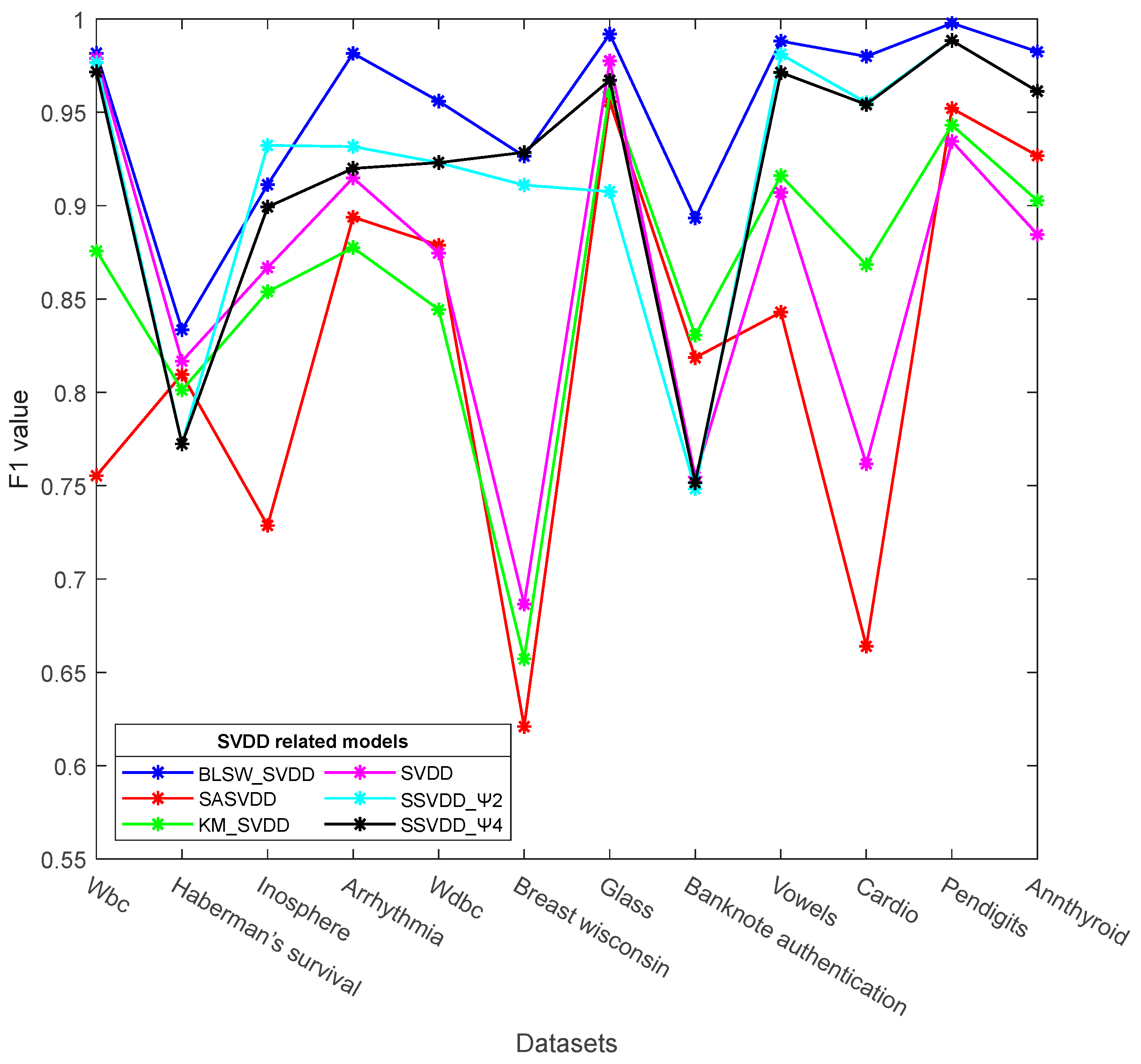
4.3. Comparison Results and Analysis with Other SVDD Models

To evaluate the performance of the proposed BLSW_SVDD model, in this section, we used 12 datasets collected from the UCI repository, described in Table 1. The BLSW_SVDD model was compared with the conventional SVDD, KM_SVDD, SA_SVDD, and SSVDD models described earlier for the experiments, and the results were compared and analyzed. In the paper of SSVDD model, the linear and nonlinear data mappings were proposed, and models Ψ1, Ψ2, Ψ3, and Ψ4 were proposed respectively depending on the regularization term Ψ, which represents the class variance in the low-dimensional space. Because the experimental results from the original study showed that the performance of SSVDD when applying linear data mappings is better than that when applying nonlinear data mappings, we used the Ψ1, Ψ2, Ψ3, and Ψ4 models corresponding to SSVDD linear mappings in the comparison experiments.

The anomaly detection accuracies of the BLSW_SVDD model proposed in this study and other SVDD comparison models on the 12 datasets are shown in

Table 3. Accuracy of different SVDD models.

	SVDD	KM_SVDD	SA_SVDD	SSVDD				BLSW_SVDD
				Ψ1	Ψ2	Ψ3	Ψ4
Wbc	0.9600	0.7913	0.8452	0.9391	0.9130	0.9478	0.9391	0.9652
Haberman’s survival	0.7011	0.6796	0.6806	0.6559	0.6774	0.6344	0.6559	0.7297
Inosphere	0.8330	0.8396	0.8340	0.8113	0.8774	0.8491	0.9151	0.8896
Arrhythmia	0.8478	0.7956	0.8309	0.8824	0.8971	0.8750	0.8456	0.9691
Wdbc	0.8215	0.7703	0.7919	0.8953	0.8953	0.8953	0.8953	0.9209
Breast Wisconsin	0.6431	0.6180	0.6900	0.7820	0.9336	0.7630	0.8294	0.9431
Glass	0.9569	0.9262	0.9169	0.8923	0.9077	0.8000	0.8154	0.9846
Banknote authentication	0.6400	0.7840	0.8049	0.6384	0.6384	0.6384	0.6165	0.8884
Vowels	0.8780	0.8654	0.9153	0.9474	0.9542	0.9497	0.9497	0.9771
Cardio	0.7382	0.7789	0.8104	0.9018	0.9164	0.9273	0.9164	0.9636
Pendigits	0.9233	0.9347	0.9455	0.9772	0.9772	0.9772	0.9772	0.9937
Annthyroid	0.8563	0.8756	0.9023	0.9255	09255	0.9255	0.9255	0.9727

. The accuracy of the BLSW_SVDD model is higher than that of other SVDD comparison models for nine datasets, and the performance is significantly better than other SVDD comparison models. For the Inosphere dataset, the SSVDD_Ψ4 model achieves a higher accuracy rate. The classification accuracy of the BLSW_SVDD model proposed in this study reaches 96% and above for 7 datasets (e.g., Vowels); for Haberman’s survival dataset with 26.4% outliers, the accuracy of the BLSW_SVDD model is lower at 72.97%, but for this dataset, the accuracy of the model proposed in this study is still higher than that of the other comparative SVDD models, which verifies the superiority of the proposed model. For the four sub-models Ψ1–Ψ4 of SSVDD, the accuracy values for these 12 datasets are not very different, but those of the SSVDD_Ψ2 and SSVDD_Ψ4 models are significantly better than those of the SSVDD_Ψ1 and SSVDD_Ψ3 models. The accuracies of the SSVDD_Ψ2 and SSVDD_Ψ4 models compared with the other four SVDD models are shown in Figure 4.

Table 4. F1 values of different SVDD models.

	SVDD	KM_SVDD	SA_SVDD	SSVDD				BLSW_SVDD
				Ψ1	Ψ2	Ψ3	Ψ4
Wbc	0.9789	0.8757	0.7554	0.9680	0.9767	0.9717	0.9717	0.9817
Haberman’s survival	0.8167	0.8013	0.8097	0.7867	0.7724	0.7724	0.7724	0.8335
Inosphere	0.8668	0.8539	0.7287	0.8529	0.9323	0.8806	0.8993	0.9112
Arrhythmia	0.9149	0.8776	0.8939	0.9163	0.9317	0.9224	0.9200	0.9816
Wdbc	0.8746	0.8443	0.8788	0.9231	0.9231	0.9231	0.9231	0.9560
Breast Wisconsin	0.6865	0.6573	0.6210	0.8678	0.9110	0.9110	0.9286	0.9265
Glass	0.9776	0.9607	0.9557	0.9421	0.9076	0.8850	0.9672	0.9919
Banknote authentication	0.7548	0.8306	0.8186	0.7410	0.7483	0.7483	0.7517	0.8933
Vowels	0.9070	0.9161	0.8430	0.9763	0.9811	0.9784	0.9713	0.9882
Cardio	0.7617	0.8683	0.6640	0.9473	0.9553	0.9604	0.9542	0.9800
Pendigits	0.9344	0.9432	0.9521	0.9885	0.9885	0.9885	0.9885	0.9977
Annthyroid	0.8846	0.9027	0.9268	0.9613	0.9613	0.9613	0.9613	0.9825

shows the F1 values of the BLSW_SVDD model and other SVDD models. The BLSW_SVDD model achieves the highest F1 measurements on 11 datasets, (e.g., Wbc). For the Inosphere dataset, the SSVDD_Ψ2 model achieves the highest F1 values. For the Wbc and Vowels datasets, the SSVDD model only achieves the second highest F1 values for the BLSW_SVDD model. For the BLSW_SVDD model proposed in this study, the F1 values reach more than 90% on 9 datasets, such as Cardio, with the corresponding F1 measurements for the Pendigits dataset reaching 99.77%. For the four sub-models of SSVDD, the SSVDD_Ψ4 model is the best-performing, followed by the SSVDD_Ψ2 model. The comparison plots of the F1 values of the SSVDD_Ψ2 and SSVDD_Ψ4 models with those of the other four SVDD models are shown in Figure 5.

In order to evaluate the performance of the BLSW_SVDD model proposed in this paper in terms of real time, we selected five representative datasets from the 12 UCI datasets mentioned above and compared the test time of the BLSW_SVDD model with other SVDD comparison models, and the test time results are shown in

Table 5. Testing time of different SVDD models.

	SVDD	KM_SVDD	SA_SVDD	SSVDD				BLSW_SVDD
				Ψ1	Ψ2	Ψ3	Ψ4
Inosphere	0.0122	0.005	0.0067	0.0026	0.0017	0.0018	0.0016	0.002
Arrhythmia	0.013	0.012	0.0152	0.0178	0.0122	0.0103	0.0101	0.0023
Breast Wisconsin	0.0034	0.0137	0.014	0.0177	0.0087	0.0079	0.0079	0.0022
Vowels	0.4157	0.0252	0.0384	0.1508	0.1422	0.1367	0.1603	0.0062
Annthyroid	15.5247	10.3347	11.3567	19.0395	18.9802	19.0092	19.0057	0.0699

. From Table 5, we can see that the test time of the BLSW_SVDD model is significantly lower than the results of the other SVDD comparison models on four datasets, and only for the Inosphere dataset, the SSVDD_Ψ4 model achieves the fastest test time. Therefore, the real-time performance of the BLSW_SVDD model proposed in this paper is significantly better than the other SVDD comparison models.

In summary, in terms of accuracy, F1 values, and real-time performance, the BLSW_SVDD model has better performance advantages than the traditional SVDD model and the improved SVDD model and has better generalization performance. However, for some datasets with a relatively large proportion of outliers, the accuracy and F1 values of the BLSW_SVDD model are not high and the detection effect is not outstanding.

5. Conclusions

Owing to problems such as the sparsity of extracted features, lack of robustness, each layer being trained greedily, and no global optimization in deep-structured neural networks, this study proposed a model for constructing reconstructed data based on BLS. Through this reconstructed model, a reconstructed error weight was introduced to SVDD to reflect the likelihood of each training data point being an anomaly sample, eliminating the problem of traditional SVDD penalizing the parameter selection. This generated a very accurate domain description with a small number of anomaly samples in the training data, which is a new reconstruction error weighted SVDD algorithm (BLSW_SVDD) proposed in this study. Experimental results indicated that the performance of the proposed BLSW_SVDD algorithm is better than the traditional SVDD and improved SVDD algorithms.

Future research can focus on the following aspects:

(1)

The kernel function used in the BLSW_SVDD model in this study is a Gaussian function, and the parameter to be optimized is $g$. However, when using kernel tricks, the SVDD algorithm faces difficulty selecting the kernel function and parameters. Therefore, in subsequent work, multiple kernel functions should be considered, which can mitigate the difficulty of selecting the kernel function and more fully portray the feature information of the original data.

(2)

The BLSW_SVDD model is ineffective on some datasets with a large proportion of abnormal data. Hence, we intend to continuously optimize the performance of the BLSW_SVDD model on datasets with a large proportion of anomaly data and continuously improve the performance of the BLSW_SVDD model to develop BLSW_SVDD model as a multi-classifier.

References

1. Tax, D.M.; Duin, R.P. Support vector domain description. Pattern Recognit. Lett. 1999, 20, 1191–1199. [Google Scholar] [CrossRef]
2. Tax, D.M.; Duin, R.P. Support vector data description. Mach. Learn. 2004, 54, 45–66. [Google Scholar] [CrossRef]
3. Qiu, K.; Song, W.; Wang, P. Abnormal data detection for industrial processes using adversarial autoencoders support vector data description. Meas. Sci. Technol. 2022, 33, 55–110. [Google Scholar] [CrossRef]
4. Karsaz, A. A modified convolutional neural network architecture for diabetic retinopathy screening using SVDD. Appl. Soft Comput. 2022, 125, 102–109. [Google Scholar] [CrossRef]
5. Lee, K.; Kim, D.-W.; Lee, D.; Lee, K.H. Improving support vector data description using local density degree. Pattern Recognit. 2005, 38, 1768–1771. [Google Scholar] [CrossRef]
6. Lee, K.; Kim, D.-W.; Lee, K.H.; Lee, D. Density-induced support vector data description. IEEE Trans. Neural Netw. 2007, 18, 284–289. [Google Scholar] [CrossRef]
7. Wang, C.-D.; Lai, J. Position regularized support vector domain description. Pattern Recognit. 2013, 46, 875–884. [Google Scholar] [CrossRef]
8. Cha, M.; Kim, J.S.; Baek, J.-G. Density weighted support vector data description. Expert Syst. Appl. 2014, 41, 3343–3350. [Google Scholar] [CrossRef]
9. Tao, H.; Yun, L.; Ke, W.; Jian, X.; Fu, L. A new weighted SVDD algorithm for outlier detection. In Proceedings of the 2016 Chinese Control and Decision Conference (CCDC), Yinchuan, China, 28–30 May 2016; pp. 5456–5461. [Google Scholar]
10. Xu, J.; Yao, J.; Ni, L. Fault detection based on SVDD and custer algorithm. In Proceedings of the 2011 International Conference on Electronics, Communications and Control (ICECC), Ningbo, China, 9–11 September 2011; pp. 2050–2052. [Google Scholar]
11. Wu, T.; Liang, Y.; Varela, R.; Wu, C.; Zhao, G.; Han, X. Self-adaptive SVDD integrated with AP clustering for one-class classification. Pattern Recognit. Lett. 2016, 84, 232–238. [Google Scholar] [CrossRef]
12. Sohrab, F.; Raitoharju, J.; Gabbouj, M.; Iosifidis, A. Subspace support vector data description. In Proceedings of the 2018 24th International Conference on Pattern Recognition (ICPR), Beijing, China, 20–24 August 2018; pp. 722–727. [Google Scholar]
13. Ruff, L.; Vandermeulen, R.; Goernitz, N.; Deecke, L.; Siddiqui, S.A.; Binder, A.; Müller, E.; Kloft, M. Deep one-class classification. In Proceedings of the International Conference on Machine Learning, Stockholm, Sweden, 10–15 July 2018; pp. 4393–4402. [Google Scholar]
14. Hojjati, H.; Armanfard, N. Dasvdd: Deep autoencoding support vector data descriptor for anomaly detection. arXiv 2021, arXiv:2106.05410. [Google Scholar]
15. Manoharan, P.; Walia, R.; Iwendi, C.; Ahanger, T.A.; Suganthi, S.; Kamruzzaman, M.; Bourouis, S.; Alhakami, W.; Hamdi, M. SVM-based generative adverserial networks for federated learning and edge computing attack model and outpoising. Expert Syst. 2022, e13072. [Google Scholar] [CrossRef]
16. Krizhevsky, A.; Sutskever, I.; Hinton, G.E. Imagenet classification with deep convolutional neural networks. Commun. ACM 2017, 60, 84–90. [Google Scholar] [CrossRef]
17. Goodfellow, I.; Bengio, Y.; Courville, A. Deep Learning; MIT Press: Cambridge, MA, USA; London, England, 2016. [Google Scholar]
18. Hinton, G.E.; Osindero, S.; Teh, Y.-W. A fast learning algorithm for deep belief nets. Neural Comput. 2006, 18, 1527–1554. [Google Scholar] [CrossRef] [PubMed]
19. Hinton, G.E.; Salakhutdinov, R.R. Reducing the dimensionality of data with neural networks. Science 2006, 313, 504–507. [Google Scholar] [CrossRef] [PubMed]
20. Salakhutdinov, R.; Larochelle, H. Efficient learning of deep boltzmann machines. In Proceedings of the Thirteenth International Conference on Artificial Intelligence and Statistics, Sardinia, Italy, 13–15 May 2010; pp. 693–700. [Google Scholar]
21. LeCun, Y.; Bottou, L.; Bengio, Y.; Haffner, P. Gradient-based learning applied to document recognition. Proc. IEEE 1998, 86, 2278–2324. [Google Scholar] [CrossRef]
22. Simonyan, K.; Zisserman, A. Very deep convolutional networks for large-scale image recognition. arXiv 2014, arXiv:1409.1556. [Google Scholar]
23. Pao, Y.-H.; Takefuji, Y. Functional-link net computing: Theory, system architecture, and functionalities. Computer 1992, 25, 76–79. [Google Scholar] [CrossRef]
24. Pao, Y.-H.; Park, G.-H.; Sobajic, D.J. Learning and generalization characteristics of the random vector functional-link net. Neurocomputing 1994, 6, 163–180. [Google Scholar] [CrossRef]
25. Kumpati, S.N.; Kannan, P. Identification and control of dynamical systems using neural networks. IEEE Trans. Neural Netw. 1990, 1, 4–27. [Google Scholar]
26. Chen, C.P.; Liu, Z. Broad learning system: A new learning paradigm and system without going deep. In Proceedings of the 2017 32nd Youth Academic Annual Conference of Chinese Association of Automation (YAC), Hefei, China, 19–21 May 2017; pp. 1271–1276. [Google Scholar]
27. Chen, C.P.; Liu, Z. Broad learning system: An effective and efficient incremental learning system without the need for deep architecture. IEEE Trans. Neural Netw. Learn. Syst. 2017, 29, 10–24. [Google Scholar] [CrossRef]
28. Chu, F.; Liang, T.; Chen, C.P.; Wang, X.; Ma, X. Weighted broad learning system and its application in nonlinear industrial process modeling. IEEE Trans. Neural Netw. Learn. Syst. 2019, 31, 3017–3031. [Google Scholar] [CrossRef]
29. Zheng, Y.; Chen, B.; Wang, S.; Wang, W. Broad learning system based on maximum correntropy criterion. IEEE Trans. Neural Netw. Learn. Syst. 2020, 32, 3083–3097. [Google Scholar] [CrossRef] [PubMed]
30. Zhang, L.; Li, J.; Lu, G.; Shen, P.; Bennamoun, M.; Shah, S.A.A.; Miao, Q.; Zhu, G.; Li, P.; Lu, X. Analysis and variants of broad learning system. IEEE Trans. Syst. Man Cybern. Syst. 2020, 52, 334–344. [Google Scholar] [CrossRef]
31. Huang, P.; Chen, B. Bidirectional broad learning system. In Proceedings of the 2020 IEEE 7th International Conference on Industrial Engineering and Applications (ICIEA), Bangkok, Thailand, 19–21 April 2020; pp. 963–968. [Google Scholar]
32. Xu, L.; Chen, C.P. Comparison and combination of activation functions in broad learning system. In Proceedings of the 2020 IEEE International Conference on Systems, Man, and Cybernetics (SMC), Toronto, ON, Canada, 11–14 October 2020; pp. 3537–3542. [Google Scholar]
33. Pu, X.; Li, C. Online semisupervised broad learning system for industrial fault diagnosis. IEEE Trans. Ind. Inform. 2021, 17, 6644–6654. [Google Scholar] [CrossRef]
34. Huang, J.; Vong, C.-M.; Chen, C.P.; Zhou, Y. Accurate and Efficient Large-Scale Multi-Label Learning With Reduced Feature Broad Learning System Using Label Correlation. IEEE Trans. Neural Netw. Learn. Syst. 2022, 1–14. [Google Scholar] [CrossRef] [PubMed]
35. Liu, B.; Zeng, X.; Tian, F.; Zhang, S.; Zhao, L. Domain transfer broad learning system for long-term drift compensation in electronic nose systems. IEEE Access 2019, 7, 143947–143959. [Google Scholar] [CrossRef]
36. Fan, J.; Wang, X.; Wang, X.; Zhao, J.; Liu, X. Incremental Wishart broad learning system for fast PolSAR image classification. IEEE Geosci. Remote Sens. Lett. 2019, 16, 1854–1858. [Google Scholar] [CrossRef]
37. Tsai, C.-C.; Hsu, C.-F.; Wu, C.-W.; Tai, F.-C. Cooperative localization using fuzzy DDEIF and broad learning system for uncertain heterogeneous omnidirectional multi-robots. Int. J. Fuzzy Syst. 2019, 21, 2542–2555. [Google Scholar] [CrossRef]
38. Vincent, P.; Larochelle, H.; Lajoie, I.; Bengio, Y.; Manzagol, P.-A.; Bottou, L. Stacked denoising autoencoders: Learning useful representations in a deep network with a local denoising criterion. J. Mach. Learn. Res. 2010, 11, 3371–3408. [Google Scholar]
39. Gong, M.; Liu, J.; Li, H.; Cai, Q.; Su, L. A multiobjective sparse feature learning model for deep neural networks. IEEE Trans. Neural Netw. Learn. Syst. 2015, 26, 3263–3277. [Google Scholar] [CrossRef]
Figure 1. The architecture of BLS.
Mathematics 10 03292 g001
Figure 2. The architecture of SVDD. Where Z denotes the test data, f ( Z ) is the decision function of the test data.
Mathematics 10 03292 g002
Figure 3. The structure of the BLS-based autoencoder.
Mathematics 10 03292 g003
Figure 4. Accuracy of different SVDD models.
Mathematics 10 03292 g004
Figure 5. F1 value of different SVDD models.
Mathematics 10 03292 g005