An Approach for Supply Chain Management Contract Selection in the Oil and Gas Industry: Combination of Uncertainty and Multi-Criteria Decision-Making Methods

Abstract

The oil and gas industry plays a significant role in the economies of many countries today. Due to various factors, including oil price fluctuations, wars, sanctions, and many other instances, selling and supplying these products at low prices is necessary. As a result, the global economy may suffer as well. Supply chain management is one way to reduce the prices of these products. This study was conducted to identify supply chain management contracts in the oil and gas industry. The paper presents an application of multi-criteria decision-making (MCDM) for coping with uncertainty. We contribute to the literature by proposing a new hybrid MCDM method with gray numbers for ranking supply chain management contracts in the oil and gas industry. The results show that the factors for evaluating supply chain management contracts must be selected, and then according to these factors, the supply chain management contracts must be chosen. As a result, we provide our customers with the best deals and help oil and gas companies minimize their costs.

1. Introduction

The oil and gas (O&G) industry is one of the most important economic sectors that contributes to a country’s income [1]. The income derived from the sector can further facilitate infrastructure construction [2]. Due to the fact that there is a level of cost involved in the extraction and maintenance of O&G, the price will increase accordingly based on the cost [3].

A supply chain refers to a chain of activities involved in transferring the raw materials from the suppliers to the end users, in which cost reduction and customer satisfaction improvement are also considered. Many companies have tried to find ways to maximize their profits through engaging in appropriate contracts [4]. The successful implementation of this is attributed to a number of factors. Therefore, to select the proper contract, factors, including both fixed and variable factors, need to be considered, such as information, human resources (HR), the time needed to purchase equipment, time, and quality, among others [5,6].

It is difficult to identify the right contractor among the many that offer various services [7]. It is imperative to consider a variety of factors before choosing a contract. Multi-criteria decision-making (MCDM) is one way to help decision-makers (DMs) make informed decisions. Decision-making based on multi-criteria is categorized into two main categories: MCDA and MODM. MCDM was used to make decisions. A pairwise comparison method and a decision matrix method are both included in MCDM. Some examples of the former include the analytic hierarchical process (AHP); network analytical process (ANP); and measuring attractiveness by categorical-based evaluation techniques (MACBETH), while some examples of the latter include: the technique for order of preference by similarity to ideal solution (TOPSIS), Vise Kriterijumska Optimizacija I Kompromisno Resenje (VIKOR), multi-objective optimization by ratio analysis plus the full multiplicative form (MULTIMOORA); and measurement of choices and ranking according to compromise solution (MARCOS), etc. The decision matrix and pairwise comparison methods were used in the research. Making decisions can be challenging in the modern world since numerous factors must be considered. The factors considered also pertain to uncertainty alternatives. Uncertainty has always been a concern for researchers. One example is using gray numbers. We will explain why gray numbers are better than fuzzy set numbers in this section [8,9].

A few papers have been published in this field; however, we look at this field from a different perspective in terms of the topic we investigate and the method we adopt. For instance, based on demand sensitivity, income distribution, and subsidy allocation to suppliers, Cai et al. [10] studied flexible supply contracts for a supply chain. There are two types of subsidies in this study: those aimed at products and those aimed at non-sold inventory. Solving these types of problems with variables involves the game theory method. Specifically, these results will assist designers in crafting contracts with the best price, the highest income distribution rate, and the least amount of inventory. Khalilpour and Karimi [11] investigated ways to reduce the purchase costs of liquid natural gas (LNG) by identifying the ways to select LNG contracts. By utilizing mixed-integer linear programming, they solved the price, duration, quality, quantity, and incoterms. To reduce the cost of purchase, these contracts must be selected based on the results of this analysis. According to Khalilpour and Karimi, the LNG contract can be selected in an uncertain environment [12]. During the evaluation of contracts, the following items were evaluated: price formula, duration, lead-time, quality, capacity, and incoterms. An uncertainty-based decision was made using mixed-integer linear programming.

We contribute to the literature by offering a new paradigm for supply chain management (SCM) agreement selection in the context of the O&G industry. The selection of an SCM contract is one of the most popular research topics, but this article is concerned with the problems brought about by the wrong contract selection. Unfortunately, few papers have been published about this subject, especially in the O&G industry. This paper also presents a novel methodology for selecting SCM contracts in the O&G industry. Finally, this paper contributes to the literature from the methodological perspective by combining MARCOS and the best–worst method (BWM) with gray numbers. The combination of these methods helps DMs make decisions in uncertain environments. To check the reliability of the results, a sensitivity analysis was performed. We have the following research questions:

RQ1—what factors should be considered to evaluate the contract to be awarded?

RQ2—which contract should be selected based on the combination of MCDM and the gray number?

This paper is structured as follows: the literature review is presented in Section 2, followed by a discussion of the research methodology in Section 3. Section 4 analyzes the data and presents the managerial implementation. The conclusion is presented in the final section.

2. Literature Review

2.1. State-of-the-Art

Selecting a SCM contract is one of the most common topics in the research area of SCM [13,14] because this is closely related to the performance of the company [15]. The existing research studies have conducted research on this topic across different economic sectors [16,17,18].

We were intrigued by Dolgui et al.’s [19] method of building a SCM contract by using blockchain and dynamic modeling. Mathematical modeling was used to determine the most effective smart contract. The Chinese blockchain was explored by Haque et al. [18] to design intelligent contracts in the oil industry’s SCM. Mohammed [19] provided an overview of the use of AHP and Delphi in the Bangladeshi SCM. The study considered several factors, including responsiveness, distortion of information, excess inventory, uncertainty, volatility of demand, and flexibility.

The selection of contracts in the water services was provided by Saravi et al. [20] under the fuzzy AHP (FAHP). Some issues were considered, including organization, management, the project’s purpose, finance, contract, and law. Following this, 18 subcategories were created based on the subdivision of each category, and then the Delphi method was used for the screening purpose. To assign a score to each contract, the FAHP software is used for grading purposes based on the performance. The efficiency of the BWM in selecting appropriate contracts was investigated by Faraji et al. [21]; the study demonstrated this for the onshore drilling projects in the oil industry. Four factors were considered: cost, environment, time, and quality.

To select the LNG contract, two methods were utilized by Yazdi et al. [22], including the mixed-integer linear programming (MILP) and the linear programming technique for multidimensional analysis of preference (LINMAP). Three factors were considered—evaporation rate, quality, and price. Based on the characteristics, the selection of a construction contract for a given project using AHP was discussed by Abdullah et al. [23]. Based on the unit prices, types of additional costs, and ten factors from the cross-sectional categories, the contracts were prioritized according to the factors and categories identified. The results show that the unit price contract was deemed the best. Several criteria were evaluated by Giri et al. [24] to select the most appropriate contract. A few factors were considered, including organization, quality, and price. In evaluating these factors, the engineering department determined the most crucial factor in selecting a particular contract.

The optimal strategy for selecting the most appropriate contract in the O&G industry can also be determined by using the ANP (Jesus et al. [25]). Four categories are outlined—the organization’s structure, the type of contract, the characteristics of the project, and the contracting process. The sub-factors reflect the specific aspects of each category. Afterward, the sub-factors within each category are prioritized by the AHP. The important contribution of contract selection to the construction industry’s success was demonstrated by Taye et al. [26]. The company status, the context of the project, and the project manager were the three factors considered. Torkayesh [17] used a hybrid approach combining the BWM with gray MARCOS to locate the most suitable locations for the disposal of healthcare waste. Initially, the locations were selected based on GIS information. Following the extraction of the factors affecting them, the BWM prioritized those factors. Lastly, they were ranked by G-MARCOS based on the factors that affected their performance. Using the gray theory and MARCOS, Badi and Pamucar ranked the supplier selection in the iron industry. To determine the validity of their method, they ranked these suppliers and then performed a sensitivity analysis. Using the hybrid MCDM methods, such as the BWM and gray MOORA, Celikbilek [20] determined which type of public transportation was the most suitable for Budapest. Fazollahtabar [21] demonstrated how to evaluate these vendors and determine the best provider. Zhang et al. [22] selected production with the intuitionistic fuzzy TODIM method. This study was conducted on a mobile phone to find the purchasing preferences and the factors that affected them. Zhang et al. [23] applied the interval fuzzy TOPSIS type 2 in the Beijing subway via utility theory. In their research, the operations risk factors were extracted and prioritized for risk reduction.

Table 1. Factors of the SCM contract selection.

References	Factor
[24,25]	Flexibility
[26,27]	Volatility of demand (not fixed demand)
[28,29]	Uncertainty (change all of the factors that are related to the contract)
[30,31]	Excess inventory
[32,33]	Distortion of information
[34,35]	Responsiveness
[36,37]	Cost
[36,38]	Quality
[39,40]	Organization
[41,42]	Contracting process
[43,44]	Project characteristics
[45,46]	Type of contract
[40,47]	Organization structure
[48,49]	Company status
[50]	Tariff and green standard

shows the factors of the contract selection (Phase I).

2.2. Research Gap

Previous studies have investigated the contract selections for different economic sectors with the application of various MCDM models. In addition, certain and uncertain situations were considered in the modeling framework of the previous studies. The following

Table 2. Methods of contract SCM selection.

References	Methods
[19]	MILP
[51]	AHP and Delphi
[42]	FAHP
[52]	BWM
[53]	MILP and LINMAP
[54]	AHP
[55]	ANP
This research	Gray number, BWM, MARCOS

summarizes the earlier studies on contract selections.

MCDM and gray numbers together make our study unique. This study adopted the BWM method, which is popular but has not received enough attention from scholars. Additionally, our proposed approach is more reliable compared to the methods used in the literature. Finally, we can apply our model to big data. Our method is more accurate than AHP. MARCOS measures the ideal–anti-ideal distances, similar to TOPSIS and VIKOR. Some advantages come with MARCOS. In some papers, the authors claimed that their results were more reliable than others. There are several advantages of gray numbers over fuzzy numbers when dealing with uncertainty. Gray numbers are based on interval data, while the membership function is used in fuzzy numbers. Gray numbers are easier to use than fuzzy ones. In gray numbers, boundaries are known because they are based on interval data or integers. The intervals between adjacent values are equal. The membership function is used for fuzzy numbers.

3. Research Methodology

3.1. Gray Number

Currently, there are a number of unknowns and unpredictable events in the business landscape. Therefore, it is extremely difficult to make informed decisions because of incomplete data. Deng developed the gray relational analysis in the 1980s [56,57]. Fuzzy numbers are not only about defining the relationship between interval data but also about determining the relationships between the membership functions [58,59], where.

Definition 1.

$${\otimes }_1\in \left[a,b\right].a_{ij}^{-}=[\frac{{\otimes }_j^{min}}{b},\frac{{\otimes }_j^{min}}{a}],\mathrm{and}{\otimes }_j^{min}=\min \left[a\right].a_{ij}^{+}=[\frac{a}{{\otimes }_j^{max}},\frac{b}{{\otimes }_j^{max}}]$$

(1)

• $a$ = is the lowest bound of data.
• $b$ = is the highest bound of data.
• ${\otimes }_1\in \left[a,b\right]$ = gray number.
• $a_{ij}^{-}$ = cost (negative) indicator,$a_{ij }^{+}$ = benefit (positive) indicator.

Definition 2.

$$x_i\left(A\right)={\displaystyle \sum }_{i=1}^n{a}_{ij}^{+}{a}_{ij}^{-}{\otimes }_j^{max}=\max \left[b\right]$$

(2)

$x_i\left(A\right)$ = reference series.

As part of the calculations, we consider the length and relative size of each gray number.

Definition 3.

Normalizing the data requires the use of the following formulas [58,59]; taking into account the benefits of (A) as described above, we arrive at the following formulas: Equations (3)–(5):

$$x_i\left(A\right)=\frac{x_i\left(A\right)-\min x_i\left(A\right)}{\max x_i\left(A\right)-\min x_i\left(A\right)}$$

(3)

$x_i\left(A\right)$= the priority of alternative i.

If there are negative factors, this formula can be applied:

$$x_i\left(A\right)=\frac{\max x_i\left(A\right)-x_i\left(A\right)}{\max x_i\left(A\right)-\min x_i\left(A\right)}$$

(4)

The following formula can be used to calculate the effects of either positive or negative factors:

$$x_i\left(A\right)=\frac{|x_i\left(A\right)-\min x_i\left(A\right)|}{\max x_i\left(A\right)-\min x_i\left(A\right)}$$

(5)

To transfer the gray number to a crisp number, the lower and higher bounds can be multiple coefficients between 0 and 1. Afterward, the average result of the lower and higher bounds, multiple to the coefficient, will be the crisp number. Regarding the coefficient, most researchers believe that the best is 0.5.

3.2. Best–Worst Method

In many parts of the world, BWM is a popular method. There are several methods for weighing the MCDM solution space. With the AHP method, fewer comparisons are needed, and the results are more accurate than those obtained from the traditional analytical hierarchy process (AHP) [60]. It is noteworthy that Rezaei [60,61] presented a method that has been applied in a variety of previous works. To implement this method, the following steps must be performed:

Step 1. The criteria and alternatives of the model are established. $C=\{c_1,c_2,\dots .,c_n$} represents the criteria of the problem; n represents the criteria’s number.

Step 2. The best and worst criteria are used to evaluate a problem.

Step 3. We compare the best criterion (B) to other criteria using a gray scale. G stands for gray. To demonstrate the best criteria, A, it is indicated as follows: $A_B=\left(G{a}_{B1},G{a}_{B2},\dots ,G{a}_{Bn}\right)$. It is obvious that $G{a}_{BB}=1$.

Step 4. In this case, the worst criterion (W) is displayed, then compared to other criteria on a scale of gray numbers, which transfers the interval data to a crisp number between 1 and 9. The following values are displayed when displaying the worst preferences for the best criterion (W): $A_w=\left(G{a}_{w1},G{a}_{w2},\dots ,G{a}_{wn}\right)$. It is obvious that $G{a}_{ww}=1$.

Step 5. The following formula is used to calculate the final weights. Specifically, they are as follows: $\left(w_1^{*},w_2^{*},\dots ,w_n^{*}\right)$.

The maximum absolute differences between $\left|\frac{w_B}{w_j}-G{a}_{Bj}\right|$ and $\left|\frac{w_j}{w_w}-G{a}_{wj}\right|$ are minimized for all j; there are various methods of calculating relative weights, including the ratio of weights. There are j criteria that must be met in each iteration, and n represents the number of iterations. The following equation illustrates how this is calculated [60,61].

$$\min \underset{j}{\max }\{\left|\frac{w_B}{w_j}-G{a}_{Bj}\right|,\left|\frac{w_j}{w_w}-G{a}_{wj}\right|\}$$

subject to:

$${\displaystyle \sum }_j{w}_j=1$$

(6)

$w_j\ge 0,$ for all j.

Another model can be rewritten as follows:

$$\min k$$

subject to:

$$\left|\frac{w_B}{w_j}-G{a}_{Bj}\right|\le k,\mathrm{for}\mathrm{all}j$$

(7)

$$\left|\frac{w_j}{w_w}-G{a}_{wj}\right|\le k,\mathrm{for}\mathrm{all}j$$

$${\displaystyle \sum }_j{w}_j=1$$

$w_j\ge 0,$ for all j.$k$ is the variable that transfers the nonlinear variable max $\left|\frac{w_B}{w_w}-G{a}_{Bj}\right|\left|\frac{w_j}{w_w}-G{a}_{wj}\right|$ to the linear variable.

3.3. MARCOS Method

Several ideal and anti-ideal methods are available in MCDA, including TOPSIS, VIKOR, etc. To locate this information, the most reliable and accurate method is to conduct a MARCOS search [62].

• Step 1: Assume that there are m alternatives and n criteria. The experts are represented by R.
• Step 2: A decision matrix is created. The row (alternatives) is represented by I, while the column (criteria) is represented by J. The first row represents the anti-ideal solution (AAI), and the second row represents the ideal solution (AI). B represents the benefit criterion, and C represents the cost criteria. $G{x}_{ij}$ demonstrates the preference of DM for criterion j and alternative i based on the gray number (G).

  $$X=\begin{array}{c}\begin{array}{c}\begin{array}{c}AAI\\ A_1\end{array}\\ \dots .\end{array}\\ A_m\\ AI\end{array}\left[\begin{array}{ccc}\begin{array}{c}G\begin{array}{cc}{x}_{aa1}& G{x}_{aa2}\end{array}\\ \begin{array}{cc}G{x}_{11}& G{x}_{12}\end{array}\end{array}& \cdots & \begin{array}{c}G{x}_{aan}\\ G{x}_{1n}\end{array}\\ ⋮& \ddots & ⋮\\ \begin{array}{c}G\begin{array}{cc}{x}_{m1}& G{x}_{22}\end{array}\\ G\begin{array}{cc}{x}_{ai1}& G{x}_{ai2}\end{array}\end{array}& \cdots & \begin{array}{c}G{x}_{mn}\\ G{x}_{ain}\end{array}\end{array}\right]$$

  (8)

  $$\mathrm{AAI}=\underset{i}{\min }G{x}_{ij}\mathrm{if}j\in B\mathrm{and}\underset{i}{\max }G{x}_{ij}\mathrm{if}j\in C$$

  $$\mathrm{AI}=\underset{i}{\max }G{x}_{ij}\mathrm{if}j\in B\mathrm{and}\underset{i}{\min }G{x}_{ij}\mathrm{if}j\in C$$
• Step 3: Matrix (X) illustrates a benefit group of criteria in conjunction with a cost group of criteria. The matrix (X) criteria are described in the following paragraphs. Normalizing the matrices produced the following results:

  $$\mathrm{N}={\left[n_{ij}\right]}_{m\times n}$$

  (9)
  • N shows the normalized matrix.
  • $n_{ij}$ is the normalized value of $G{x}_{ij}$
  $$n_{ij}=\frac{G{x}_{ai}}{G{x}_{ij}}\mathrm{if}j\in C$$

  (10)

  $$n_{ij}=\frac{G{x}_{ij}}{G{x}_{ai}}\mathrm{if}j\in B$$

  (11)

  Matrix X consists of the $G{x}_{ij}$ and $G{x}_{ai}$ alternatives. m is the number of alternatives and n is the number of criteria.
• Step 4: Let V be a matrix whose weight is a multiple of a matrix. The following formula illustrates this concept. $w_j$ are the weights of the criteria.

  $$v_{ij}=n_{ij}\times w_j$$

  (12)
• Step 5: A utility degree is a measure of the usefulness of an alternative $K_i$. Hence, it is essential to note that the utilities of the ideal and anti-ideal alternatives are calculated as follows:

  $$K_i^{-}=\frac{S_i}{S_{aai}}$$

  (13)

  $$K_i^{+}=\frac{S_i}{S_{ai}}$$

  (14)

  S_i (i = 1, 2, …, n). The following provides a summary of the alternative to the weighted matrix V.

  $$S_i={\displaystyle \sum }_{i=1}^n{v}_{ij}$$

  (15)
  • $S_{aai}$ is the alternative to the weighted matrix V for the alternative anti-ideal.
  • $S_{ai}$ is the alternative to the weighted matrix V for the alternative ideal.
• Step 6: There is a utility function f($K_i$), in which the alternatives are described in terms of their utilities. The ideal and anti-ideal alternatives can be used to derive the utility functions. The utility function can be derived as follows.

  $$f(K_i)=\frac{K_i^{+}+K_i^{-}}{1+\frac{1-f\left(K_i^{+}\right)}{f\left(K_i^{+}\right)}+\frac{1-f\left(K_i^{-}\right)}{f\left(K_i^{-}\right)}}$$

  (16)

  There is a utility function $f\left(K_i^{-}\right)$ for the AAI; this is demonstrated by the utility function $f\left(K_i^{+}\right)$ for the AI. The final utility functions related to the ideal and AAI are as follows:

  $$f(K_i^{+})=\frac{K_i^{-}}{K_i^{+}+K_i^{-}}$$

  (17)

  $$f(K_i^{-})=\frac{K_i^{+}}{K_i^{+}+K_i^{-}}$$

  (18)
• Step 7: Using the final utility scores, we calculated the ranking. In the utility function ranking, the functions with the highest scores are considered the top [62].

3.4. Customized Critical Success Factors (CSF)s (Phase II)

Several methods are available for screening the factors. As a result of its ease of customization, Delphi is one of the most popular methods for DMs.

There is a debate regarding the number of DMs. Most researchers recommend that a study has five to fifteen participants. In individual studies, the number of participants should range from five to one hundred [63,64,65]. There are approximately eight DMs involved in this study [65]. Below is a table with additional study information. The term “DM” refers to an individual with a university degree in SCM and at least 25 years of experience. The following table (

Table 3. DMs’ Information.

DMs	Experience	Certificate
1	26	PhD
2	28	MA
3	29	BSc
4	31	PhD
5	27	MA
6	26	BSc
7	28	PhD
8	29	MA

) provides information about the DMs.

The extracted factors were used to design a questionnaire. This questionnaire was reviewed by the DMs. A five-point scale was used to rate the answers. The factors, as shown in

Table 4. Results of customized factors.

	DM1	DM2	DM3	DM4	DM5	DM6	DM7	DM8	Average	Accept/Reject
Flexibility	4	5	4	5	4	5	4	5	4.5	Accept
Volatility of demand	5	4	3	5	4	5	3	4	4.125	Accept
Uncertainty	5	4	5	4	3	5	4	5	4.375	Accept
Tariff	3	4	5	3	3	4	3	4	3.625	Reject
Excess inventory	3	5	4	5	3	5	4	5	4.25	Accept
Distortion of information	3	4	5	3	4	4	5	3	4	Accept
Responsiveness	5	4	5	5	4	5	4	5	4.625	Accept
Cost	5	5	5	4	5	4	5	4	4.625	Accept
Quality	5	4	5	3	5	4	5	4	4.375	Accept
Organization	5	4	5	4	5	4	5	3	4.375	Accept
Contracting process	5	4	5	4	5	3	5	4	4.375	Accept
Green standard	4	4	4	3	4	5	3	3	3.75	Reject
Project characteristics	4	5	4	5	4	5	4	5	4.5	Accept
Type of contract	5	5	5	4	3	5	3	4	4.25	Accept
Organization structure	3	4	3	5	4	5	3	5	4	Accept

, were screened. Factors were accepted if they had average scores of four or above.

The contract factors in the O&G industry must be customized because of geography and other relevant conditions; hence, the Delphi method was used. In this method, the related questionnaire has questions in the format of a five-point Likert scale. If the average score of each item is equal to or more than 4, it will be accepted, otherwise, it will be rejected. As mentioned in the above table, the average scores of two factors were less than 4; hence, these factors were eliminated. Among the fifteen factors, two factors were eliminated, and the other thirteen factors remained.

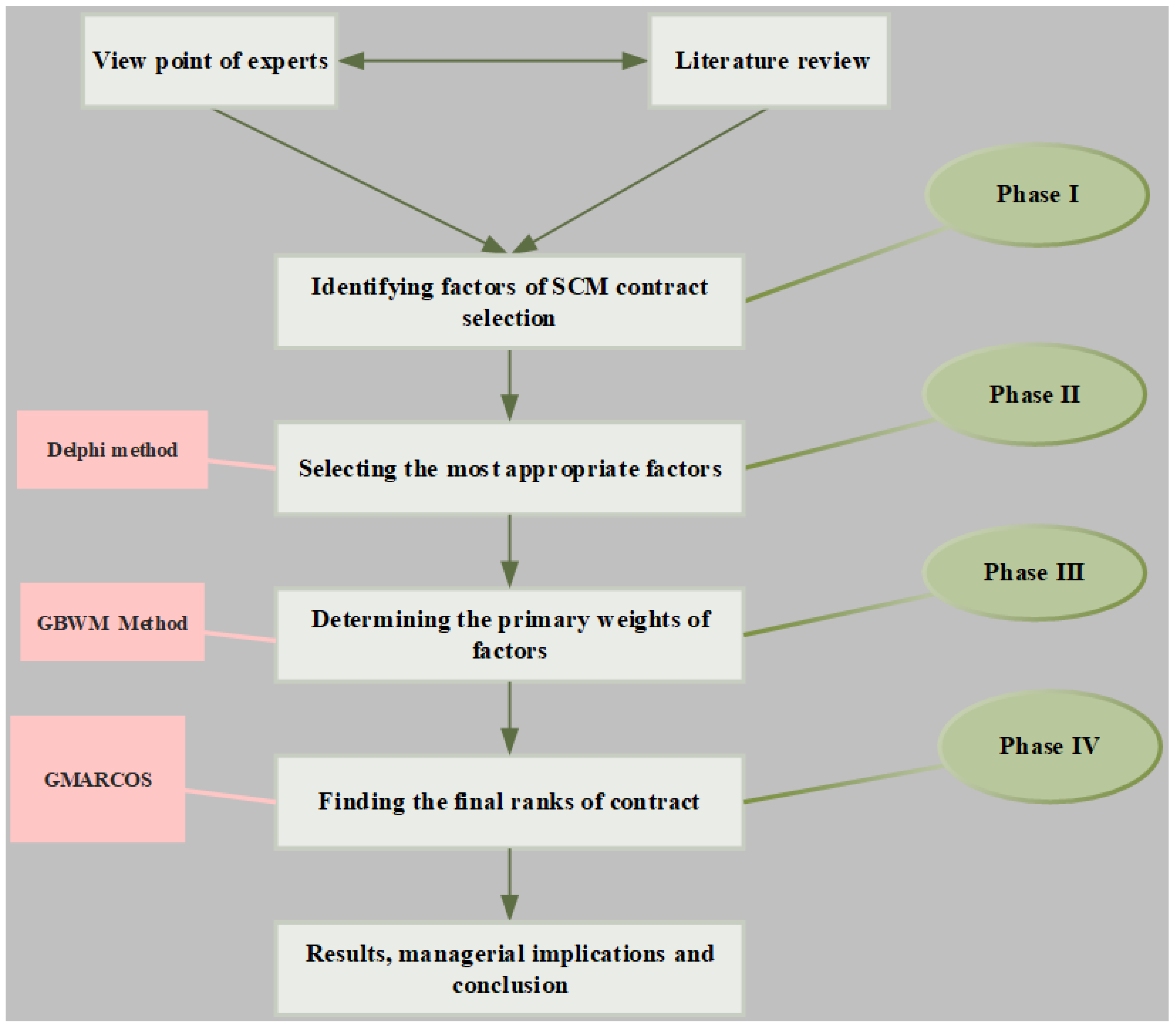
3.5. Research Procedure

Previous studies have uncovered several factors relevant to this paper’s topic; still, each country’s circumstances must be taken into account. It is common to use the Delphi method, but several other methods are available. A pair-wise comparison method known as BWM was used to determine the primary weights. Due to the unpredictable nature of the real world, gray numbers were used. Contracts were ranked using the gray MARCOS method, which belongs to the family of ideal and anti-ideal methods. The ranking enables DM to determine which contract to select based on related factors.

Figure 1 shows the research procedure.

4. Data Analysis

4.1. GBWM (Best–Worst Method with Gray Numbers) Analysis (Phase III)

After the implementation of phase I (i.e., customizing the factors by the Delphi method), the BWM was applied to find the primary weights. Since the MARCOS method needed a primary weight, GBWM was applied. This section is related to phase II.

The BWM was applied after the best criterion was chosen in the first place. Then, the questionnaire was designed accordingly based on the criterion; in the questionnaire, the nine-point Likert scale was used to indicate the DM preferences. The average preferences of the DMs were considered to rank both the best and the worst criteria.

The gray linguistic scale is defined in the first step.

Table 5. Linguistic variables (data from Muneeb et al. [66], Kaviani et al. [67]).

Gray Number	Verbal Linguistics
[0–1]	Least Important
[1–2]	Very very low importance
[2–3]	Very low importance
[3–4]	Low importance
[4–5]	Moderate
[5–6]	High importance
[6–7]	Very high importance
[7–8]	Very very high importance
[8–9]	Most important

shows the linguistics variables.

Quality is the most crucial factor in determining the best criteria. Therefore, how the DMs allocated their preferences based on quality is illustrated in

Table 6. Best criteria DMs’ preferences.

Criteria	Flexibility	Volatility of Demand	Uncertainty	Excess Inventory	Distortion of Information	Responsiveness	Cost	Organization	Contracting Process	Project Characteristics	Type of Contract	Organization Structure
Quality	[7.2–7.8]	[6.4–6.6]	[6.2–6.8]	[8.3–8.8]	[6.3–6.6]	[7.5–7.7]	[8.3–8.9]	[5.2–5.7]	[6.2–6.5]	[7.3–7.4]	[7.2–7.8]	[6.3–6.6]
Crisp number	7.5	6.5	6.5	8.55	6.45	7.6	8.6	5.45	6.35	7.35	7.5	6.45

.

Table 7. Worst criteria, DM preferences.

Criteria	Cost	Crisp Number
Flexibility	[4.2–4.7]	4.45
Volatility of demand	[3.2–3.8]	3.5
Uncertainty	[6.1–6.7]	6.4
Excess inventory	[3.3–3.8]	3.55
Distortion of information	[3.2–3.6]	3.4
Responsiveness	[4.5–4.8]	4.65
Quality	[5.3–5.9]	5.6
Organization	[3.2–3.6]	3.4
Contracting process	[7.2–7.9]	7.55
Project characteristics	[7.4–7.6]	7.5
Type of contract	[7.3–7.6]	7.45
Organization structure	[4.2–4.9]	4.55

shows that based on the preference of the DMs, when selecting a replacement, the cost criterion is treated as the worst criterion.

Therefore, the transformation from gray numbers to crisp numbers was achieved. In this case, the lower bound was transferred to the coefficient, which also applied to the upper bound. More specifically, the values of the coefficient ranged from 0 to 1. Based on the previous studies, the most appropriate coefficient was 0.5.

Then, based on Equations (6) and (7) and Table 6 and Table 7, the linear problem of BWM was created. This model was solved by the LINGO V22 software.

Min z = $k$.

Subject to:

$$\begin{gathered} -k\times m_1\le m_8-7.5\times m_1\le k\times m_1 \\ -k\times m_2\le m_8-6.5\times m_2\le k\times m_2 \\ -k\times m_3\le m_8-6.5\times m_3\le k\times m_3 \\ -k\times m_4\le m_8-8.55\times m_4\le k\times m_4 \\ -k\times m_5\le m_8-6.45\times m_5\le k\times m_5 \\ -k\times m_6\le m_8-7.6\times m_6\le k\times m_6 \\ -k\times m_7\le m_8-8.6\times m_7\le k\times m_7 \\ -k\times m_9\le m_8-5.45\times m_9\le k\times m_9 \\ -k\times m_{10}\le m_8-6.35\times m_{10}\le k\times m_{10} \\ -k\times m_{11}\le m_8-7.35\times m_{11}\le k\times m_{11} \\ -k\times m_{12}\le m_8-7.5\times m_{12}\le k\times m_{12} \\ -k\times m_{13}\le m_8-6.45\times m_{13}\le k\times m_{13} \\ -k\times m_7\le m_1-4.45\times m_7\le k\times m_7 \\ -k\times m_7\le m_2-3.5\times m_7\le k\times m_7 \\ -k\times m_7\le m_3-6.4\times m_7\le k\times m_7 \\ -k\times m_7\le m_4-3.35\times m_7\le k\times m_7 \\ -k\times m_7\le m_5-3.4\times m_7\le k\times m_7 \\ -k\times m_7\le m_6-4.65\times m_7\le k\times m_7 \\ -k\times m_7\le m_8-5.6\times m_7\le k\times m_7 \\ -k\times m_7\le m_9-3.4\times m_7\le k\times m_7 \\ -k\times m_7\le m_{10}-7.55\times m_7\le k\times m_7 \\ -k\times m_7\le m_{11}-7.5\times m_7\le k\times m_7 \\ -k\times m_7\le m_{12}-7.45\times m_7\le k\times m_7 \\ -k\times m_7\le m_{13}-7.55\times m_7\le k\times m_7 \\ {m}_1+m_2+m_3+m_4+m_5+m_6+m_7+m_8+m_9+m_{10}+m_{11}+m_{12}+m_{13}=1 \\ {m}_1,m_2,m_3,m_4,m_5,m_6,m_7,m_8,m_9,m_{10},m_{10},m_{10},m_{10}>0 \\ k>0 \end{gathered}$$

(19)

k represents the transferring $\underset{j}{\max }\{\left|\frac{w_B}{w_j}-G{a}_{Bj}\right|,\left|\frac{w_j}{w_w}-G{a}_{wj}\right|\}$. For instance, in the equation above, we have 13 criteria from m₁ to m₁₃. In the first section of the above equation, m₈ is the best criterion, and m₇ is the worst criterion.

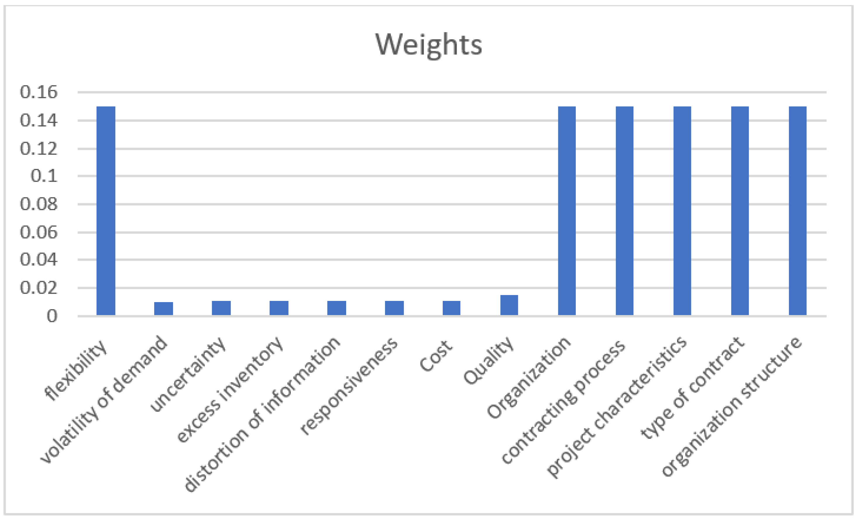
The results (according to Equation (19)) show the weight of each factor. Figure 2 shows these weights. The sum of these factors must be 1 and each criterion has its weight.

Suppose that the consistency rate of 6.5 was used—we notice that this problem was very consistent.

To rank the contracts, the GMARCOS (MARCOS with gray numbers) method was implemented. This study presents the results in the context of the O&G industry, in which there were seven contracts suggested; the one that must be offered is shown in this study.

4.2. Independency Relationship among Factors

The condition that needs to be met before ranking the contract is that the factors must be independent of each other.

To determine this, we used the gray analysis.

A represents an alternative and C represents a specific criterion.

Table 8. Decision matrix of the gray relational analysis (GRA).

	C1	C2	C3	C4	C5	C6	C7	C8	C9	C10	C11	C12	C13
A1	6.5	5.6	7.75	8.7	8.6	6.6	7.55	8.25	7.45	7.6	5.75	7.45	8.3
A2	7.6	7.55	6.5	6.5	7.55	6.8	8.6	8.3	6.8	8.6	8.3	8.7	7.75
A3	7.75	8.3	7.6	7.55	8.6	8.7	6.5	6.8	6.5	8.7	7.55	8.3	7.45
A4	8.7	8.6	8.6	7.6	7.75	6.5	7.45	8.6	6.5	8.3	7.6	8.7	6.5
A5	6.5	6.8	6.5	6.8	8.6	8.6	8.65	8.3	7.75	6.5	7.55	6.5	8.6
A6	8.7	6.5	8.7	7.55	7.6	7.45	6.5	8.7	8.3	8.6	7.45	7.55	8.3
A7	8.6	7.55	6.5	8.7	8.3	7.6	6.8	6.5	8.3	6.8	7.55	8.6	8.7
min	6.5	5.6	6.5	6.5	7.75	6.5	6.5	6.5	6.5	6.5	5.75	6.5	6.5
max	8.7	8.6	8.7	8.7	8.6	8.7	8.65	8.7	8.3	8.7	8.3	8.7	8.7
max-min	2.2	3	2.2	2.2	1.05	2.2	2.15	2.2	1.8	2.2	2.55	2.2	2.2
star	7.7	7.6	7.7	7.7	7.6	7.7	7.65	7.7	7.3	7.7	7.3	7.7	7.7

F_ij is the criterion, and A_i is the alternative. The star is the highest value of each criterion.

shows the decision matrix of the gray rational analysis.

According to Equations (1) and (2),

Table 9. Dimensionless decision matrix.

	C1	C2	C3	C4	C5	C6	C7	C8	C9	C10	C11	C12	C13
A1	0.71	0.61	0.88	1	1	0.73	0.86	0.94	0.88	0.86	0.65	0.84	0.95
A2	0.86	0.86	0.71	0.71	0.86	0.75	0.99	0.95	0.79	0.99	1	1	0.88
A3	0.88	0.96	0.86	0.85	1	1	0.72	0.75	0.75	1	0.9	0.95	0.84
A4	1	1	0.99	0.86	0.89	0.71	0.84	0.99	0.75	0.95	0.9	1	0.71
A5	0.71	0.76	0.71	0.75	1	0.99	1	0.95	0.92	0.71	0.9	0.71	0.99
A6	1	0.72	1	0.85	0.87	0.84	0.72	1	1	0.99	0.88	0.85	0.95
A7	0.99	0.86	0.71	1	0.96	0.86	0.76	0.71	1	0.75	0.9	0.99	1

shows the dimensionless decision matrix.

The GRA coefficient is calculated by normalizing the data using Equations (3)–(5).

Table 10. Normalized matrix.

	C1	C2	C3	C4	C5	C6	C7	C8	C9	C10	C11	C12	C13
A1	0.29	0.39	0.12	0	0	0.27	0.14	0.06	0.12	0.14	0.35	0.16	0.05
A2	0.14	0.14	0.29	0.29	0.14	0.25	0.01	0.05	0.21	0.01	0	0	0.12
A3	0.12	0.04	0.14	0.15	0	0	0.28	0.25	0.25	0	0.1	0.05	0.16
A4	0	0	0.01	0.14	0.11	0.29	0.16	0.01	0.25	0.05	0.1	0	0.29
A5	0.29	0.24	0.29	0.25	0	0.01	0	0.05	0.08	0.29	0.1	0.29	0.01
A6	0	0.28	0	0.15	0.13	0.16	0.28	0	0	0.01	0.12	0.15	0.05
A7	0.01	0.14	0.29	0	0.04	0.14	0.24	0.29	0	0.25	0.1	0.01	0
Δmin	0	0	0	0	0	0	0	0	0	0	0	0	0
Δmax	0.29	0.39	0.29	0.29	0.14	0.29	0.28	0.29	0.25	0.29	0.35	0.29	0.29
rΔmax	0.14	0.2	0.14	0.14	0.07	0.14	0.14	0.14	0.12	0.14	0.17	0.14	0.14
Δmin + rΔmax	0.14	0.2	0.14	0.14	0.07	0.14	0.14	0.14	0.12	0.14	0.35	0.16	0.05

r demonstrates the correlation of GRA. Δmin is the lowest value of the criterion. Δmax is the highest value of the criterion. r is the coefficient of the gray number. Many researchers believe that the best coefficient is 0.5. if Δmin + rΔmax is less than 0.5, it means that there is no relationship in that criterion.

shows the normalized matrix.

When we ensured that there were no relationships among these criteria, the MARCOS method was applied. In

Table 11. Initial decision matrix.

	Flexibility	Volatility of Demand	Uncertainty	Excess Inventory	Distortion of Information	Responsiveness	Cost	Quality	Organization	Contracting Process	Project Characteristics	Type of Contract	Organization Structure
Contract 1	[6.2–6-8]	[5.4–5.8]	[7.6–7.9]	[8.5–8.9]	[8.4–8.8]	[6.4–6.8]	[7.4–7.7]	[8.1–8.4]	[7.3–7.6]	[7.3–7.9]	[5.6–5.9]	[7.3–7.6]	[8.1–8.5]
Contract 2	[7.4–7.8]	[7.4–7.7]	[6.4–6.6]	[6.2–6-8]	[7.3–7.8]	[6.7–6.9]	[8.4–8.8]	[8.1–8.5]	[6.7–6.9]	[8.4–8.8]	[8.1–8.5]	[8.5–8.9]	[7.6–7.9]
Contract 3	[7.6–7.9]	[8.1–8.5]	[7.4–7.8]	[7.3–7.8]	[8.4–8.8]	[8.5–8.9]	[6.4–6.6]	[6.7–6.9]	[6.2–6-8]	[8.5–8.9]	[7.4–7.7]	[8.1–8.5]	[7.3–7.6]
Contract 4	[8.5–8.9]	[8.4–8.8]	[8.4–8.8]	[7.4–7.8]	[7.6–7.9]	[6.4–6.6]	[7.3–7.6]	[8.4–8.8]	[6.4–6.6]	[8.1–8.5]	[7.4–7.8]	[8.5–8.9]	[6.2–6-8]
Contract 5	[6.2–6-8]	[6.7–6.9]	[6.4–6.6]	[6.7–6.9]	[8.4–8.8]	[8.4–8.8]	[8.5–8.8]	[8.1–8.5]	[7.6–7.9]	[6.2–6-8]	[7.3–7.8]	[6.4–6.6]	[8.4–8.8]
Contract 6	[8.5–8.9]	[6.4–6.6]	[8.5–8.9]	[7.4–7.7]	[7.4–7.8]	[7.3–7.6]	[6.2–6.8]	[8.5–8.9]	[8.1–8.5]	[8.4–8.8]	[7.3–7.6]	[7.3–7.8]	[8.1–8.5]
Contract 7	[8.4–8.8]	[7.3–7.8]	[6.2–6-8]	[8.5–8.9]	[8.1–8.5]	[7.4–7.8]	[6.7–6.9]	[6.4–6.6]	[8.1–8.5]	[6.7–6.9]	[7.4–7.7]	[8.4–8.8]	[8.5–8.9]

, the first decision matrix was created.

4.3. GMARCOS Analysis (Phase IV)

The decision matrix based on DM preferences, reflected by the gray number, was created in the first step. The DMs told their preferences (according to Table 5). Moreover, these preferences were the means of all DM preferences. Table 11 shows the initial decision matrix.

Table 12. Crisp decision matrix. + represents benefit criteria and – demonstrates cost criteria.

	Flexibility	Volatility of Demand	Uncertainty	Excess Inventory	Distortion of Information	Responsiveness	Cost	Quality	Organization	Contracting Process	Project Characteristics	Type of Contract	Organization Structure
	+	−	−	+	−	+	−	+	+	+	+	+	+
AAI	6.5	8.6	8.7	6.5	8.6	6.5	8.65	6.5	6.5	6.5	5.75	6.5	6.5
Contract 1	6.5	5.6	7.75	8.7	8.6	6.6	7.55	8.25	7.45	7.6	5.75	7.45	8.3
Contract 2	7.6	7.55	6.5	6.5	7.55	6.8	8.6	8.3	6.8	8.6	8.3	8.7	7.75
Contract 3	7.75	8.3	7.6	7.55	8.6	8.7	6.5	6.8	6.5	8.7	7.55	8.3	7.45
Contract 4	8.7	8.6	8.6	7.6	7.75	6.5	7.45	8.6	6.5	8.3	7.6	8.7	6.5
Contract 5	6.5	6.8	6.5	6.8	8.6	8.6	8.65	8.3	7.75	6.5	7.55	6.5	8.6
Contract 6	8.7	6.5	8.7	7.55	7.6	7.45	6.5	8.7	8.3	8.6	7.45	7.55	8.3
Contract 7	8.6	7.55	6.5	8.7	8.3	7.6	6.8	6.5	8.3	6.8	7.55	8.6	8.7
AI	8.7	5.6	6.5	8.7	7.55	8.7	6.5	8.7	8.3	8.7	8.3	8.7	8.7

shows the crisp decision matrix. The crisp data were obtained by multiplying the low and high bounds by 0.5 and then taking the average. The plus sign indicates the benefit criteria, whereas the minus sign indicates the cost criteria. AAI is the least (preference) of that criterion and AI is the largest score of that criterion if that criterion is a benefit (positive). If it is a cost criterion (negative), the computations of AAI and AI are vice-versa of the benefit criterion.

To normalize the initial matrix, Equations (8)–(10) were applied. To normalize numbers if the criterion was a benefit, this score is divided with AI, but if the criterion is a cost, the score is divided with AAI.

Table 13. Normalized decision matrix. + represents benefit criteria and – demonstrates cost criteria.

	Flexibility	Volatility of Demand	Uncertainty	Excess Inventory	Distortion of Information	Responsiveness	Cost	Quality	Organization	Contracting Process	Project Characteristics	Type of Contract	Organization Structure
Kind of criterion	+	−	−	+	−	+	−	+	+	+	+	+	+
Weights	0.15	0.01	0.011	0.011	0.011	0.011	0.011	0.015	0.15	0.15	0.15	0.15	0.15
AAI	0.747	0.651	0.747	0.747	0.878	0.747	0.751	0.747	0.783	0.747	0.693	0.747	0.747
Contract 1	0.747	1.000	0.839	1.000	0.878	0.759	0.861	0.948	0.898	0.693	0.693	0.856	0.954
Contract 2	0.874	0.742	1.000	0.747	1.000	0.782	0.756	0.954	0.819	1.000	1.000	1.000	0.891
Contract 3	0.891	0.675	0.855	0.868	0.878	1.000	1.000	0.782	0.783	0.910	0.910	0.954	0.856
Contract 4	1.000	0.651	0.756	0.874	0.974	0.747	0.872	0.989	0.783	0.916	0.916	1.000	0.747
Contract 5	0.747	0.824	1.000	0.782	0.878	0.989	0.751	0.954	0.934	0.910	0.910	0.747	0.989
Contract 6	1.000	0.862	0.747	0.868	0.993	0.856	1.000	1.000	1.000	0.898	0.898	0.868	0.954
Contract 7	0.989	0.742	1.000	1.000	0.910	0.874	0.956	0.747	1.000	0.910	0.910	0.989	1.000
AI	1.000	1.000	1.000	1.000	1.000	1.000	1.000	1.000	1.000	1.000	1.000	1.000	1.000

shows the normalized decision matrix.

The introduction of multiple weights converts the normalized matrix to a weighted matrix, as reflected by Equation (11). After normalizing the score, the weights, which are obtained from the BWM, are multiple in the normalized matrix to obtain the weighted matrix.

Table 14. Weighted decision matrix. + represents benefit criteria and – demonstrates cost criteria.

	Flexibility	Volatility of Demand	Uncertainty	Excess Inventory	Distortion of Information	Responsiveness	Cost	Quality	Organization	Contracting Process	Project Characteristics	Type of Contract	Organization Structure
	+	−	-	+	−	+	−	+	+	+	+	+	+
AAI	0.112	0.007	0.008	0.008	0.010	0.008	0.008	0.011	0.117	0.112	0.104	0.112	0.112
Contract 1	0.112	0.010	0.009	0.011	0.010	0.008	0.009	0.014	0.135	0.104	0.104	0.128	0.143
Contract 2	0.131	0.007	0.011	0.008	0.011	0.009	0.008	0.014	0.123	0.150	0.150	0.150	0.134
Contract 3	0.134	0.007	0.009	0.010	0.010	0.011	0.011	0.012	0.117	0.136	0.136	0.143	0.128
Contract 4	0.150	0.007	0.008	0.010	0.011	0.008	0.010	0.015	0.117	0.137	0.137	0.150	0.112
Contract 5	0.112	0.008	0.011	0.009	0.010	0.011	0.008	0.014	0.140	0.136	0.136	0.112	0.148
Contract 6	0.150	0.009	0.008	0.010	0.011	0.009	0.011	0.015	0.150	0.135	0.135	0.130	0.143
Contract 7	0.148	0.007	0.011	0.011	0.010	0.010	0.011	0.011	0.150	0.136	0.136	0.148	0.150
AI	0.150	0.010	0.011	0.011	0.011	0.011	0.011	0.015	0.150	0.150	0.150	0.150	0.150

shows the weighted decision matrix.

Based on Equations (12)–(17), we determined the final ranking of the contracts.

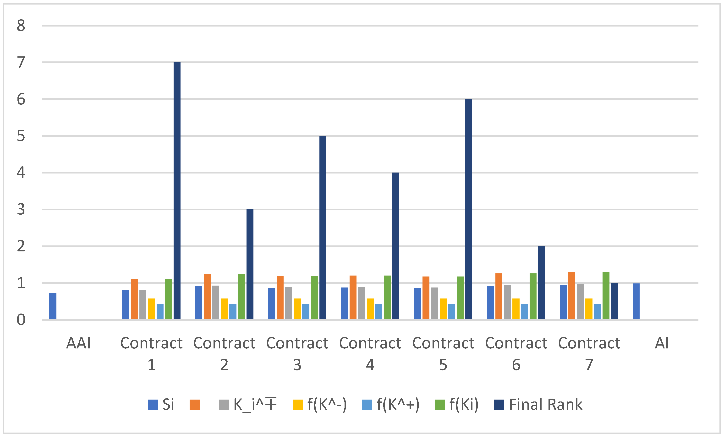
In the first step, the utilities of the ideal and anti-ideal of contracts were computed according to Equations (12) and (13). S_i is the summary of the weighted matrix according to Equation (14). f($K^{+})$ is the utility function of the IS(ideal solution), and f($K^{-})$ is related to the AIS (anti-ideal solution). Then, according to f(K_i), the contracts are ranked. Figure 3 shows the final weight.

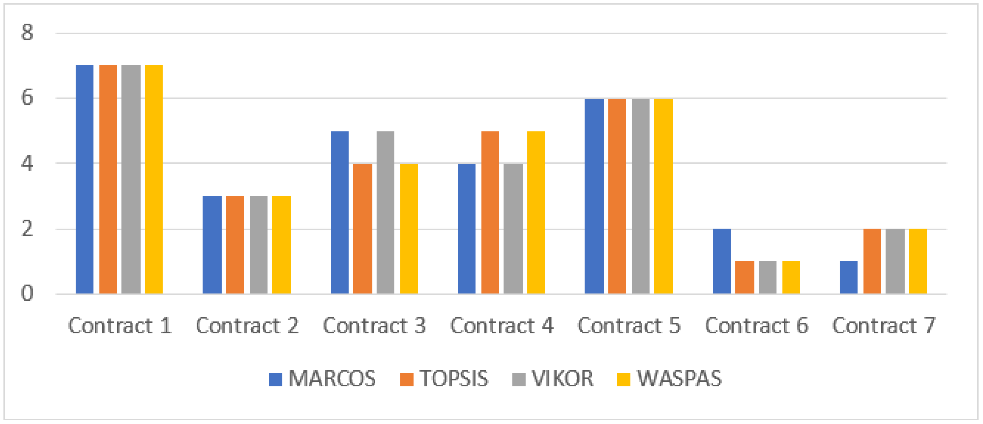
4.4. Comparative Analysis

This section mainly assesses the reliability of the results by comparing the findings derived from our method and the ones from TOPSIS, VIKOR, and WASPAS. These models belong to the family of the ideal and anti-ideal methods.

Hence, they were selected to compare with the results from our model to determine the robustness of this method. Figure 4 shows the results from different MCDM methods.

Table 15. Spearman test.

MARCOS	TOPSIS	VIKOR	WASPAS
Co-efficient	0.929	0.964	0.929
p-value	0.003	0	0.003

shows the results of the Spearman test, which examined the correlation between the MARCOS method and the other methods mentioned above. If the P-value of the test is less than 0.01 and the coefficient is close to 1, our results have a higher degree of reliability.

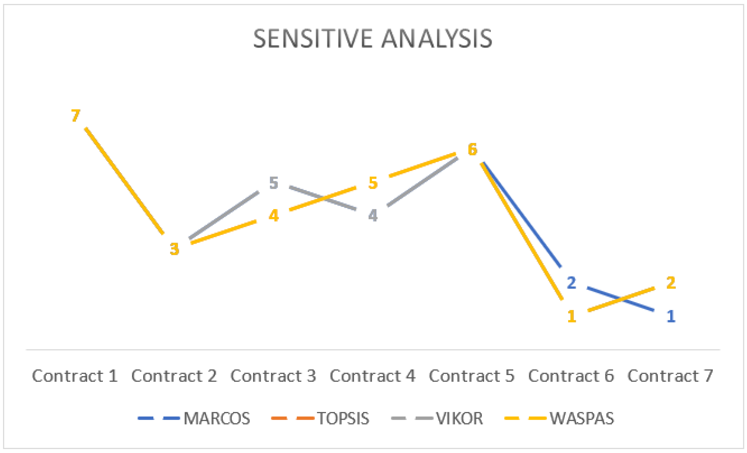
When a study’s p-value is less than 5%, it shows that it is statistically significant. We performed the sensitivity analysis, the results of which are presented in Figure 5.

5. Conclusions and Managerial Implementation

We used a hybrid method of MCDM, including the BWM and MARCOS, to investigate the contract selection of SCM in the context of the O&G sector. The proposed method is supposed to increase the reliability of the results. Our world is characterized by uncertainty, which affects the reliability of the decision-making process. The gray number, which is one of the methods used to deal with uncertainty, carries several benefits compared to the fuzzy set.

Collecting the previously studied factors was the first step to answering our first research question; the factors were screened and customized by the Delphi technique. Based on the results, we eliminated two factors, and thirteen factors remained. To address our second question, we used a hybrid of GBWM and GMARCOS to assess seven contracts. Based on the results, contract seven was chosen.

Furthermore, among the 13 factors, we found that the following factors were the most important: flexibility, organizational structure, type of contract, project characteristics, the contracting process, and organization. The results of our sensitivity analysis show that our results are reliable and robust.

This hybrid method has some advantages. First, it helps managers to select the best (and most suitable) contracts. Each item in the O&G industry, such as extraction, refining, and transportation, concluded the contracts for SCM. With this model, by finding the best contract, the cost and lead time of SCM decrease, and customer satisfaction (and so forth) increase. In addition, our results are robust because we compared them with the results of another similar method (showing that the results have a relationship). Finally, this model is a general model that can be used in different industries, although the factors must be customized with a specific industry and the SCM contract.

These results have designed a road map for DMs regarding contract selection in industries. This hybrid method shows how to select a contract in the O&G industry, considering essential and crucial related factors. The results show which contract (among the seven contracts) must be selected (according to crucial factors). The selected contract will decrease the cost of the project, increase customer satisfaction, and optimize resource allocations.

The current study suffers from some limitations. For instance, due to the issue of confidentiality, we had limited access to the contracts. In addition, we faced difficulties in accessing the second-level DMs because of their busy schedules and lack of availability. Other fuzzy methods can be used in future research, such as D-number, Z-number, etc. Furthermore, these fuzzy methods can be used with the MCDM method, and the related results can be compared with the ones from the current study.

References

1. Youssouf, M.A.L.I. Effects of World Oil Price Movement on Macroeconomic Performance in Saudi ARABIA. 2019. Available online: http://psasir.upm.edu.my/id/eprint/83078/ (accessed on 15 July 2022).
2. Bradshaw, M.; van de Graaf, T.; Connolly, R. Preparing for the new oil order? Saudi Arabia and Russia. Energy Strateg. Rev. 2019, 26, 100374. [Google Scholar] [CrossRef]
3. Hamilton, J.D. What is an oil shock? J. Econom. 2003, 113, 363–398. [Google Scholar] [CrossRef]
4. Yazdi, A.K.; Wanke, P.F.; Hanne, T.; Bottani, E. A decision-support approach under uncertainty for evaluating reverse logistics capabilities of healthcare providers in Iran. J. Enterp. Inf. Manag. 2020, 33, 991–1022. [Google Scholar] [CrossRef]
5. Yazdi, A.K.; Wanke, P.F.; Hanne, T.; Abdi, F.; Sarfaraz, A.H. Supplier selection in the oil & gas industry: A comprehensive approach for Multi-Criteria Decision Analysis. Socioecon. Plann. Sci. 2021, 79, 101142. [Google Scholar]
6. Poberschnigg, T.F.d.; Pimenta, M.L.; Hilletofth, P. How can cross-functional integration support the development of resilience capabilities? The case of collaboration in the automotive industry. Supply Chain Manag. Int. J. 2020, 25, 789–801. [Google Scholar] [CrossRef]
7. Governatori, G.; Idelberger, F.; Milosevic, Z.; Riveret, R.; Sartor, G.; Xu, X. On legal contracts, imperative and declarative smart contracts, blockchain systems. Artif. Intell. Law 2018, 26, 377–409. [Google Scholar] [CrossRef]
8. Bakhat, R.; Rajaa, M. Developing a novel Grey integrated multi-criteria approach for enhancing the supplier selection procedure: A real-world case of Textile Company. Decis. Sci. Lett. 2019, 8, 211–224. [Google Scholar] [CrossRef]
9. Aggarwal, S.; Srivastava, M.K. A grey-based DEMATEL model for building collaborative resilience in supply chain. Int. J. Qual. Reliab. Manag. 2019. [Google Scholar] [CrossRef]
10. Cai, J.; Hu, X.; Tadikamalla, P.R.; Shang, J. Flexible contract design for VMI supply chain with service-sensitive demand: Revenue-sharing and supplier subsidy. Eur. J. Oper. Res. 2017, 261, 143–153. [Google Scholar] [CrossRef]
11. Khalilpour, R.; Karimi, I.A. Selection of liquefied natural gas (LNG) contracts for minimizing procurement cost. Ind. Eng. Chem. Res. 2011, 50, 10298–10312. [Google Scholar] [CrossRef]
12. Khalilpour, R.; Karimi, I.A. Contract selection under uncertainty: LNG buyers’ perspective. In Computer Aided Chemical Engineering; Elsevier: Amsterdam, The Netherlands, 2012; Volume 31, pp. 1487–1491. [Google Scholar]
13. Elabed, S.; Shamayleh, A.; Daghfous, A. Sustainability-oriented innovation in the health care supply chain. Comput. Ind. Eng. 2021, 160, 107564. [Google Scholar] [CrossRef]
14. Behnke, K.; Janssen, M. Boundary conditions for traceability in food supply chains using blockchain technology. Int. J. Inf. Manag. 2020, 52, 101969. [Google Scholar] [CrossRef]
15. Bocek, T.; Stiller, B. Smart contracts—Blockchains in the wings. In Digital Marketplaces Unleashed; Springer: Berlin/Heidelberg, Germany, 2018; pp. 169–184. [Google Scholar]
16. Shermin, V. Disrupting governance with blockchains and smart contracts. Strateg. Chang. 2017, 26, 499–509. [Google Scholar] [CrossRef]
17. Hu, K.-J.; Vincent, F.Y. An integrated approach for the electronic contract manufacturer selection problem. Omega 2016, 62, 68–81. [Google Scholar] [CrossRef]
18. Walter, J. Safety management at the frontier: Cooperation with contractors in oil and gas companies. Saf. Sci. 2017, 91, 394–404. [Google Scholar] [CrossRef]
19. Dolgui, A.; Ivanov, D.; Potryasaev, S.; Sokolov, B.; Ivanova, M.; Werner, F. Blockchain-oriented dynamic modelling of smart contract design and execution in the supply chain. Int. J. Prod. Res. 2020, 58, 2184–2199. [Google Scholar] [CrossRef]
20. Çelikbilek, Y.; Moslem, S.; Duleba, S. A combined grey multi criteria decision making model to evaluate public transportation systems. Evol. Syst. 2022, 1–15. [Google Scholar] [CrossRef]
21. Fazlollahtabar, H.; Kazemitash, N. Green supplier selection based on the information system performance evaluation using the integrated Best-Worst Method. Facta Univ. Ser. Mech. Eng. 2021, 19, 345–360. [Google Scholar] [CrossRef]
22. Zhang, Z.; Guo, J.; Zhang, H.; Zhou, L.; Wang, M. Product selection based on sentiment analysis of online reviews: An intuitionistic fuzzy TODIM method. Complex Intell. Syst. 2022, 8, 3349–3362. [Google Scholar] [CrossRef]
23. Zhang, Z.; Zhao, X.; Qin, Y.; Si, H.; Zhou, L. Interval type-2 fuzzy TOPSIS approach with utility theory for subway station operational risk evaluation. J. Ambient Intell. Humaniz. Comput. 2021, 1–15. [Google Scholar] [CrossRef]
24. Li, J.; Luo, X.; Wang, Q.; Zhou, W. Supply chain coordination through capacity reservation contract and quantity flexibility contract. Omega 2021, 99, 102195. [Google Scholar] [CrossRef]
25. Farahani, M.H.; Dawande, M.; Gurnani, H.; Janakiraman, G. Better to Bend than to Break: Sharing Supply Risk Using the Supply-Flexibility Contract. Manuf. Serv. Oper. Manag. 2021, 23, 1257–1274. [Google Scholar] [CrossRef]
26. Kantari, L.A.; Pujawan, I.N.; Arvitrida, N.I.; Hilletofth, P. Mixing contract-based and on-demand sourcing of transportation services for improved supply chain performance under supply uncertainties. Int. J. Syst. Sci. Oper. Logist. 2021, 1–17. [Google Scholar] [CrossRef]
27. Avinadav, T.; Chernonog, T.; Meilijson, I.; Perlman, Y. A consignment contract with revenue sharing between an app developer and a distribution platform. Int. J. Prod. Econ. 2022, 243, 108322. [Google Scholar] [CrossRef]
28. Yucekaya, A. Electricity trading for coal-fired power plants in Turkish power market considering uncertainty in spot, derivatives and bilateral contract market. Renew. Sustain. Energy Rev. 2022, 159, 112189. [Google Scholar] [CrossRef]
29. Farsi, M.; Erkoyuncu, J.A. An agent-based approach to quantify the uncertainty in Product-Service System contract decisions: A case study in the machine tool industry. Int. J. Prod. Econ. 2021, 233, 108014. [Google Scholar] [CrossRef]
30. Li, Y.; Deng, S.; Zhang, Y.; Liu, B. Coordinating the retail supply chain with item-level RFID and excess inventory under a revenue-cost-sharing contract. Int. Trans. Oper. Res. 2021, 28, 1505–1525. [Google Scholar] [CrossRef]
31. Chakraborty, A.; Verma, N.K.; Chatterjee, A.K. A Single Supplier Multi Buyer Supply Chain Coordination under Vendor-managed Inventory: Ensuring Buyers’ Interests in a Decentralized Setting. IIM Kozhikode Soc. Manag. Rev. 2022, 22779752211072936. [Google Scholar] [CrossRef]
32. Clark, A.; Reggiani, G. Contracts for acquiring information. arXiv 2021, arXiv:2103.03911. [Google Scholar]
33. Zhang, J.; Qi, L.; Tong, S. Dynamic contract under quick response in a supply chain with information asymmetry. Prod. Oper. Manag. 2021, 30, 1273–1289. [Google Scholar] [CrossRef]
34. Ebekozien, A.; Aigbavboa, C.; Nwaole, A.N.C.; Dako, E.O.; Awo-Osagie, A.I. Quantity surveyor’s ethical responsiveness on construction projects: Issues and solutions. Int. J. Build. Pathol. Adapt. 2021. [Google Scholar] [CrossRef]
35. Aïd, R.; Possamaï, D.; Touzi, N. Optimal electricity demand response contracting with responsiveness incentives. Math. Oper. Res. 2022. [Google Scholar] [CrossRef]
36. Akin, F.D.; Polat, G.; Turkoglu, H.; Damci, A. A crashing-based time-cost trade-off model considering quality cost and contract clauses. Int. J. Constr. Manag. 2021, 1–10. [Google Scholar] [CrossRef]
37. Samanta, B.; Giri, B.C. A two-echelon supply chain model with price and warranty dependent demand and pro-rata warranty policy under cost sharing contract. Decis. Mak. Appl. Manag. Eng. 2021, 4, 47–75. [Google Scholar] [CrossRef]
38. Lee, J.H.; Mistur, E.; Liu, L.; Ashuri, B. Determining contract requirements for quality assurance program in innovative project delivery. In Proceedings of the Construction Research Congress 2022, Arlington, VA, USA, 9–12 March 2022; pp. 179–188. [Google Scholar]
39. Bugrov, O.; Bugrova, O. Formalization of Selection of Contract-Organizational Project Delivery Strategy. 2018. Available online: https://iopscience.iop.org/article/10.1088/1755-1315/304/3/032001/meta (accessed on 10 July 2022).
40. Cheaitou, A.; Larbi, R.; Al Housani, B. Decision making framework for tender evaluation and contractor selection in public organizations with risk considerations. Socioecon. Plann. Sci. 2019, 68, 100620. [Google Scholar] [CrossRef]
41. Ni, J.; Zhao, J.; Chu, L.K. Supply contracting and process innovation in a dynamic supply chain with information asymmetry. Eur. J. Oper. Res. 2021, 288, 552–562. [Google Scholar] [CrossRef]
42. Sarvari, H.; Chan, D.W.M.; Ashrafi, B.; Olawumi, T.O.; Banaitiene, N. Prioritization of Contracting Methods for Water and Wastewater Projects Using the Fuzzy Analytic Hierarchy Process Method. Energies 2021, 14, 7815. [Google Scholar] [CrossRef]
43. Novikov, S.V.; Dmitriev, O.N. Vision of genesis of presentation of Hi-Tech project during competitive selection. Russ. Eng. Res. 2018, 38, 320–322. [Google Scholar] [CrossRef]
44. Ding, J.; Zhai, W.; Wang, Z.; Zhang, K.; Cai, J. Modelling and Design Analysis of Contract Payment Methods in Civil Engineering Projects. In Proceedings of the IOP Conference Series: Earth and Environmental Science, Moscow, Russia, 27 May–6 June 2019; Volume 304, p. 32001. [Google Scholar]
45. Camci, A.; Çimen, Ö.; Gül, S. Selection of contract type in construction projects using spherical AHP method. In Proceedings of the International Online Conference on Intelligent Decision Science, Istanbul, Turkey, 7–8 August 2020; pp. 531–547. [Google Scholar]
46. Zhou, Y.-W.; Lin, X.; Zhong, Y.; Xie, W. Contract selection for a multi-service sharing platform with self-scheduling capacity. Omega 2019, 86, 198–217. [Google Scholar] [CrossRef]
47. Zhao, X.; Gu, B.; Gao, F.; Chen, S. Matching model of energy supply and demand of the integrated energy system in coastal areas. J. Coast. Res. 2020, 103, 983–989. [Google Scholar] [CrossRef]
48. Carbonara, N.; Pellegrino, R. Public-private partnerships for energy efficiency projects: A win-win model to choose the energy performance contracting structure. J. Clean. Prod. 2018, 170, 1064–1075. [Google Scholar] [CrossRef]
49. Ruml, A.; Qaim, M. Effects of marketing contracts and resource-providing contracts in the African small farm sector: Insights from oil palm production in Ghana. World Dev. 2020, 136, 105110. [Google Scholar] [CrossRef]
50. Toktaş-Palut, P. An integrated contract for coordinating a three-stage green forward and reverse supply chain under fairness concerns. J. Clean. Prod. 2021, 279, 123735. [Google Scholar] [CrossRef]
51. Mohammed, H.J. The optimal project selection in portfolio management using fuzzy multi-criteria decision-making methodology. J. Sustain. Financ. Investig. 2021, 1–17. [Google Scholar] [CrossRef]
52. Faraji, A.; Rashidi, M.; Khadir, P.; Perera, S. A Risk Analysis-Best Worst Method Based Model for Selection of the Most Appropriate Contract Strategy for Onshore Drilling Projects in the Iranian Petroleum Industry. Buildings 2021, 11, 97. [Google Scholar] [CrossRef]
53. KarbassiYazdi, A.; Rashidi Komijan, A.; Raissi, S.; Modiri, M. A robust model for supplying LNG from different contracts considering overall and incremental discount options. Energy Sources, Part A Recover. Util. Environ. Eff. 2021, 43, 1805–1824. [Google Scholar] [CrossRef]
54. Abdullah, A.K.; Alshibani, A. Multi-criteria decision-making framework for selecting sustainable private partners for housing projects. J. Financ. Manag. Prop. Constr. 2021. [Google Scholar] [CrossRef]
55. de Jesus, V.M.; Gomes, L.F.A.M.; Filardi, F. The Selection of Oil & Gas Projects Contract Strategies with the ANP: A Case Study. Indep. J. Manag. Prod. 2019, 10, 355–379. [Google Scholar]
56. Deng, J.L. Grey system fundamental method. Huazhong Univ. Sci. Technol. Wuhan China 1982. [Google Scholar]
57. Julong, D. Introduction to grey system theory. J. Grey Syst. 1989, 1, 1–24. [Google Scholar]
58. Pawlak, Z.; Wong, S.K.M.; Ziarko, W. Rough sets: Probabilistic versus deterministic approach. Int. J. Man. Mach. Stud. 1988, 29, 81–95. [Google Scholar] [CrossRef]
59. Pawlak, Z. Rough Sets: Theoretical Aspects of Reasoning about Data Kluwer Academic Publishers; Springer Science & Business Media: Dordrecht, The Netherlands, 1991. [Google Scholar]
60. Rezaei, J. Best-worst multi-criteria decision-making method. Omega 2015, 53, 49–57. [Google Scholar] [CrossRef]
61. Rezaei, J. Best-worst multi-criteria decision-making method: Some properties and a linear model. Omega 2016, 64, 126–130. [Google Scholar] [CrossRef]
62. Stević, Ž.; Pamučar, D.; Puška, A.; Chatterjee, P. Sustainable supplier selection in healthcare industries using a new MCDM method: Measurement of alternatives and ranking according to COmpromise solution (MARCOS). Comput. Ind. Eng. 2020, 140, 106231. [Google Scholar] [CrossRef]
63. Dalkey, N.; Helmer, O. An experimental application of the Delphi method to the use of experts. Manage. Sci. 1963, 9, 458–467. [Google Scholar] [CrossRef]
64. Schmidt, R.C. Managing Delphi surveys using nonparametric statistical techniques. Decis. Sci. 1997, 28, 763–774. [Google Scholar] [CrossRef]
65. Kennedy, H.P. Enhancing Delphi research: Methods and results. J. Adv. Nurs. 2004, 45, 504–511. [Google Scholar] [CrossRef]
66. Muneeb, F.M.; Yazdi, A.K.; Wanke, P.; Yiyin, C.; Chughtai, M. Critical success factors for sustainable entrepreneurship in Pakistani Telecommunications industry: A hybrid grey systems theory/best-worst method approach. Manag. Decis. 2020, 58, 2565–2591. [Google Scholar] [CrossRef]
67. Kaviani, M.A.; Yazdi, A.K.; Ocampo, L.; Kusi-Sarpong, S. An integrated grey-based multi-criteria decision-making approach for supplier evaluation and selection in the oil and gas industry. Kybernetes 2019, 49, 406–441. [Google Scholar] [CrossRef]
Figure 1. Research methodology.
Mathematics 10 03230 g001
Figure 2. The final weight of BWM.
Mathematics 10 03230 g002
Figure 3. Final weight.
Mathematics 10 03230 g003
Figure 4. The results from different MCDM methods.
Mathematics 10 03230 g004
Figure 5. Sensitive analysis.
Mathematics 10 03230 g005