An Optimal Random Hybrid Maintenance Policy of Systems under a Warranty with Rebate and Charge

Abstract

Facilitated by advanced digital technologies, reliability managers can monitor system working cycles during the whole life cycle. Such a technological realization can help reliability managers ensure system reliability in real time by monitoring working cycles. In this paper, by incorporating a limited random working cycle, rebate and charge into warranty theory, a random free repair warranty with rebate and charge (RFRW-RC) is devised to ensure system reliability during the warranty stage. Under RFRW-RC, the rebate removes manufacturers’ responsibility for continuing to ensure system reliability, while the charge is a support where manufacturers continue to ensure system reliability. The warranty cost of RFRW-RC is derived, and a random discrete free repair warranty (RDFRW) is presented by simplifying RFRW-RC. By mixing random age replacement last (RARL) and classic age replacement (CAR), a random hybrid age replacement (RHAR) is designed in order to ensure system reliability during the post-warranty stage. In such an RHAR, RARL is applied to extend the replacement time during the post-warranty stage in order to maximize the remaining life of the system through warranty, and CAR is used to lower the maintenance cost of the system through warranty. The cost rate of RHAR is modeled, and the cost rate of RDFRW is offered as well by discussing parameter values. The decision variable is optimized by minimizing the cost rate model. The properties of the presented models are explored from numerical perspectives.

1. Introduction

The reliability guarantee of the system is a key component of the system life cycle management. From the viewpoint of the operation and maintenance, the reliability guarantee of the system could be classified into the reliability guarantee during the warranty stage and the reliability guarantee during the post-warranty stage. Usually, the warrantor or manufacturer is in charge of the reliability guarantee during the warranty stage, and the warrantee or user is responsible for the reliability guarantee during the post-warranty stage.

From the perspective of the manufacturer, many warranty policies (models) have been studied to guarantee system reliability during the warranty stage. Depending on the maintenance method, the warranty policies of existing works can be divided into three categories of research. The first category of research is to design classic warranty policies, wherein the first failure time of the system is characterized as a distribution function (this field has been presented in Refs. [1,2,3]), and classic maintenance technologies (repair, replacement or preventive maintenance) are used to ensure the system reliability. This category of warranty can be found in Refs. [4,5,6,7,8,9,10,11]. Under the support of random maintenance policies in Refs. [12,13,14,15], the second category of research aims at modeling random warranty policies where random working cycles were incorporated into warranty theory. For example, by incorporating random working cycles into a renewing pro-rate replacement warranty (RPRW), Ref. [16] designed a two-dimensional random renewing pro-rate replacement warranty with a refund (2DRRPRW with R) where a partial refund is used to maintain fairness; Ref. [17] designed the two-dimensional free repair warranty first (2DFRWF) and two-dimensional renewing free repair warranty last (2DFRWL) by incorporating limited random working cycles into the warranty period; Ref. [18] integrated limited random working cycles into the warranty period and designed the two-dimensional renewing free replacement warranty first (2DRFRWF) and two-dimensional renewing free replacement warranty last (2DRFRWL). The third category of research is to design condition-based warranty policies by means of a stochastic process in Refs. [19,20,21,22,23,24,25,26,27,28], which can be found in Refs. [29,30,31]. Further classification and details on warranty policies can be found in Refs. [32,33].

To guarantee system reliability during the post-warranty stage, many maintenance policies have been modeled from the viewpoint of the consumer. Occasionally, this type of policy is called a post-warranty maintenance policy. Similar to the classification of warranty policies, the post-warranty maintenance policies of existing works can be divided into three types of research. Under the assumption that the first failure time of the system is modeled as a distribution function, the first type of research is to model the post-warranty maintenance policies by means of classic maintenance technologies, which have been presented in Refs. [34,35,36,37]. The second type of research is to devise random post-warranty maintenance policies by incorporating random working cycles into the post-warranty stage, which have been provided in Refs. [38,39,40,41]. The objective of the third type of research is to devise condition-based post-warranty maintenance policies, wherein system deterioration is characterized as a stochastic process. For example, Ref. [42] designed a condition-based post-warranty maintenance policy by assuming that a stochastic process can characterize deterioration process.

For a multi-limitation warranty, the case at which the warranty expires is multidimensional. Under a multi-limitation warranty, if a warranty limitation is reached early, then the warrantee related to this situation could perceive that they is treated unfairly because their warranty service period is shorter than each of the warranty service periods produced by other warranty limitations. If the rebate in Refs. [43,44] is offered to this type of warrantee, then the warrantee’s unfairness can be removed, and the warrantor disrupts responsibility for continuing to ensure system reliability. Under a multi-limitation warranty, if a warranty limitation is reached last, then the warranty cost absorbed by the warrantor is greater than the warranty cost produced by the case where a warranty limitation is reached earlier. If the warrantor charges the warrantee whose warranty expiry occurs last, then the warrantor can recover warranty costs, and the system reliability is further ensured by the warrantor. However, rebates and charges have seldom been used to handle the above problem.

After consulting the literature on post-warranty maintenance policies, it is found that post-warranty maintenance policies are seldom designed based on the difference of system ages. Under a multi-limitation warranty, the different warranty limitations produce different system ages. For a system through a multi-limitation warranty, if its age is greater, then its reliability function becomes lower. According to reliability theory, this fact signals that the maintenance cost during the post-warranty stage will be greater. Conversely, if its age is smaller, then its reliability function is still higher. Such a fact signals that the longer remaining life during the post-warranty stage has not been used. These results imply that under a multi-limitation warranty, how to reduce the maintenance cost of an older system and to maximally use the longer remaining life of a younger system is a problem that must be solved. However, scholars and practitioners have not yet solved this problem.

In this paper, by incorporating a limited random working cycle, a rebate, a charge and minimal repair into the warranty stage, a random free repair warranty with rebate and charge (RFRW-RC) is designed to ensure system reliability during the warranty stage, wherein the rebate maintains fairness and disrupts manufacturers’ responsibility for continuing to ensure system reliability, while the charge is a support where manufacturers continue to ensure system reliability. The warranty cost of RFRW-RC is derived, and the related special model is obtained. By incorporating random age replacement last (RARL) in Refs. [15,17] and classic age replacement (CAR) into the post-warranty stage, a random hybrid age replacement (RHAR) is modeled to ensure system reliability during the post-warranty stage, wherein RARL is applied to extend the replacement time during the post-warranty stage so as to maximally use the remaining life during the post-warranty stage and CAR is used to lower the maintenance cost during the post-warranty stage. The cost rate of RHAR is modeled, and special cost rates are also offered by discussing parameter values. The decision variable is optimized by minimizing the cost rate of RHAR. From a numerical perspective, the properties of the presented models are explored, and insights are found.

The organization of this paper is listed below. Section 2 defines a novel warranty model, derives a warranty cost model and presents a special warranty model. In Section 3, a random maintenance model is established to ensure system reliability during the post-warranty stage. Similarly, Section 3 presents the conditions for the existence and uniqueness of the optimal solution. Section 4 explores the properties of the proposed models and performs sensitivity analysis on some key parameters. Section 5 concludes the paper.

2. Warranty Models

Similar to Refs. [15,38], the assumptions used are listed as follows: the system performs projects at working cycles, and the working cycles $Y_i$ of the $i\mathrm{th}$ ($i=1,2,\dots$) project are random working cycles that are independent and obey an identical distribution function $G(y)=\mathrm{Pr}\{Y_i<y\}$, wherein memory does not exist; the first failure time $X$ obeys the distribution function $F(x)=\mathrm{Pr}\{X<x\}$, whose failure rate function is $r(u)$; and the time to repair or replacement is negligible.

2.1. Warranty Model Definition

Denote a time span and the number of random working cycles by $w$ and $n$ ($0<n<\infty$), respectively; let $S_n$ be the working time, where the $n\mathrm{th}$ random working cycle is completed by the system, where $S_n={\displaystyle \sum _{i=1}^n{Y}_i}$; then, a warranty is defined below.

• The expiry of the warranty service is triggered by the $n\mathrm{th}$ random working cycle completion.
• If the $n\mathrm{th}$ random working cycle is completed before the end of the time span $w$, the warrantor will provide the warrantee with a rebate related to the shortage time $w-S_n$.
• If the $n\mathrm{th}$ random working cycle is still not completed until the end of the time span $w$, the warrantee will be charged a fee related to the excess time $S_n-w$ to ensure system reliability during the time span $(w,\hspace{1em}{S}_n-w]$. Here, such a fee is named a charge.
• The system is minimally repaired at each failure before the expiry of the warranty, and the warrantor absorbs the cost of each minimal repair. Here, such a cost is named the repair cost.

Because both rebate and charge are considered in such a warranty, this warranty is named a random free repair warranty with rebate and charge (RFRW-RC), which can be explained concisely by Figure 1.

Notes: ① When the $n\mathrm{th}$ random working cycle is completed before the end of the time span $w$, the warrantor provides the related warrantee with a rebate to remove the responsibility for continuing to ensure the system reliability during the interval $(S_n,w]$; such a rebate can remove the unfairness of the warrantee whose warranty expires earlier. ② When the $n\mathrm{th}$ random working cycle is still not completed by the end of the time span $w$, by charging a fee from the related warrantee, the warrantor is responsible for continuing to guarantee the system reliability during the interval $(w,S_n]$. ③ The case in which RFRW-RC expires includes two types, which are “RFRW-RC expires at the $n\mathrm{th}$ random working cycle completion before the time span $w$” and “RFRW-RC expires at the $n\mathrm{th}$ random working cycle completion after the time span $w$”.

2.2. Warranty Cost Model

RFRW-RC requires that the system is minimally repaired at failure before the $n\mathrm{th}$ random working cycle completes. Denote the unit repair cost by $c_m$. Then, according to reliability theory, until the $n\mathrm{th}$ random working cycle is completed before the end of the time span $w$, the total repair cost $C_1(S_m)$ of the warrantor can be computed as

$$C_1(S_n)=c_m{\displaystyle {\int }_0^{S_n}r(u)\mathrm{d}u}$$

(1)

where $S_n<w$.

RFRW-RC signals that when the $n\mathrm{th}$ random working cycle is completed before the end of the time span $w$, the warrantor needs to offer a rebate that is dependent on the shortage time $w-S_n$. This implies that such a rebate can be characterized as a function with respect to the variable $w-S_n$. Such a rebate function can be denoted with respect to the variable $w-S_n$ by $R(S_n)$. Then, such a rebate function $R(S_n)$ is modeled as

$$R(S_n)=a{\left(1-S_n/w\right)}^b{c}_m{\displaystyle {\int }_{S_n}^{w}r(u)\mathrm{d}u}$$

(2)

where $S_n<w$, $a>0$ and $b>0$.

By summing Equations (1) and (2), the total cost $T{C}_1(S_m)$ under the case where the $n\mathrm{th}$ random working cycle is completed before the end of the time span $w$ can be represented by

$$T{C}_1(S_m)=C_1(S_n)+R(S_n)=c_m{\displaystyle {\int }_0^{S_n}r(u)\mathrm{d}u}+a{\left(1-S_n/w\right)}^b{c}_m{\displaystyle {\int }_{S_n}^{w}r(u)\mathrm{d}u}$$

(3)

By Ref. [45], the working time $S_n$ is a random variable whose distribution function $G^{(n)}(s)$ and reliability function ${\overline{G}}^{(n)}(s)$ are modeled as Stieltjes convolution $G^{(n)}(s)=\mathrm{Pr}\left\{S_n<s\right\}={\displaystyle {\int }_0^s{G}^{(n-1)}(s-u)\mathrm{d}G(u)}$ and Stieltjes convolution ${\overline{G}}^{(n)}(s)=\mathrm{Pr}\left\{S_n>s\right\}=1-{\displaystyle {\int }_0^s{G}^{(n-1)}(s-u)\mathrm{d}G(u)}$, respectively. When the $n\mathrm{th}$ random working cycle completes before the end of the time span $w$, the system’s warranty service period equates to the working time $S_n$, where $S_n<w$. Furthermore, such a working time $S_n$ is subject to the distribution function $H(s)$ as

$$H(s)=\mathrm{Pr}\left\{S_n<s|S_n<w\right\}=\mathrm{Pr}\left\{S_n<s\right\}/\mathrm{Pr}\left\{S_n<w\right\}=G^{(n)}(s)/G^{(n)}(w)$$

(4)

where $0<s<w$.

By means of the distribution function $H(s)$ in Equation (4), the total cost $T{C}_1(S_n)$ can be rewritten as

$$ET{C}_1={\displaystyle {\int }_0^{w}T{C}_1(s)\mathrm{d}H(s)}=c_m{\displaystyle {\int }_0^w\left({\displaystyle {\int }_0^{s}r(u)\mathrm{d}u}+a{\left(1-s/w\right)}^b{\displaystyle {\int }_s^{w}r(u)\mathrm{d}u}\right)\mathrm{d}{G}^{(n)}(s)}/G^{(n)}(w)$$

(5)

As indicated in RFRW-RC, when the $n\mathrm{th}$ random working cycle is completed after the end of the time span $w$, the warrantee provides a charge to the warrantor. Such a charge depends on the excess time $S_n-w$. In other words, this charge alike is characterized as a function with respect to the variable $S_n-w$. Let $P(S_n)$ be a charge function with respect to the variable $S_n-w$. Then, the charge function $P(S_n)$ is modeled as

$$P(S_n)=\alpha {\left(1+w/\left(S_n-w\right)\right)}^{\beta }\times c_m{\displaystyle {\int }_w^{S_n}r(u)\mathrm{d}u}$$

(6)

where $S_n>w$, $\alpha >0$ and $\beta >0$.

Similarly, according to reliability theory, until the $n\mathrm{th}$ random working cycle is completed after the end of the time span $w$, the total repair cost $C_2(S_n)$ of the warrantor can be computed as

$$C_2(S_n)=c_m{\displaystyle {\int }_0^{S_n}r(u)\mathrm{d}u}$$

(7)

where $S_n>w$, which is different from $S_n<w$ in Equation (1).

By algebraic operation on Equations (6) and (7), the total cost $T{C}_2(S_n)$ under the case where the $n\mathrm{th}$ random working cycle is completed after the end of the time span $w$ can be represented by

$$T{C}_2(S_n)=C_2(S_n)-P(S_n)=c_m\left({\displaystyle {\int }_0^{S_n}r(u)\mathrm{d}u}-\alpha {\left(1+w/\left(S_n-w\right)\right)}^{\beta }{\displaystyle {\int }_w^{S_n}r(u)\mathrm{d}u}\right)$$

(8)

When the $n\mathrm{th}$ random working cycle is completed after the end of the time span $w$, the system’s warranty service period equates to the working time $S_n$, where $S_n>w$. Such a working time $S_n$ obeys the distribution function $I(s)$ as

$$I(s)=\mathrm{Pr}\left\{S_n<s|S_n>w\right\}=\mathrm{Pr}\left\{S_n<s\right\}/\mathrm{Pr}\left\{S_n>w\right\}=G^{(n)}(s)/{\overline{G}}^{(n)}(w)$$

(9)

where $s>w$.

By means of the distribution function $I(s)$ in Equation (9), the total cost $T{C}_2(S_n)$ can be rewritten as

$$ET{C}_2={\displaystyle {\int }_w^{\infty }T{C}_2(s)\mathrm{d}I(s)}=c_m{\displaystyle {\int }_w^{\infty }\left({\displaystyle {\int }_0^{s}r(u)\mathrm{d}u}-\alpha {\left(1+w/\left(s-w\right)\right)}^{\beta }{\displaystyle {\int }_w^{s}r(u)\mathrm{d}u}\right)\mathrm{d}{G}^{(n)}(s)}/{\overline{G}}^{(n)}(w)$$

(10)

Because the probabilities that the $n\mathrm{th}$ random working cycle is completed before or after the end of the time span $w$ are represented by $G^{(n)}(w)$ and ${\overline{G}}^{(n)}(w)$, the warranty cost $TWC$ of RFRW-RC can be derived as

$$\begin{array}{l}TWC=G^{(n)}(w)\times ET{C}_1+{\overline{G}}^{(n)}(w)\times ET{C}_2\\ =c_m\left({\displaystyle {\int }_0^w\left({\displaystyle {\int }_0^{s}r(u)\mathrm{d}u}+a{\left(1-s/w\right)}^b{\displaystyle {\int }_s^{w}r(u)\mathrm{d}u}\right)\mathrm{d}{G}^{(n)}(s)}+{\displaystyle {\int }_w^{\infty }\left({\displaystyle {\int }_0^{s}r(u)\mathrm{d}u}-\alpha {\left(1+w/\left(s-w\right)\right)}^{\beta }{\displaystyle {\int }_w^{s}r(u)\mathrm{d}u}\right)\mathrm{d}{G}^{(n)}(s)}\right)\\ =c_m\left({\displaystyle {\int }_0^{\infty }\left({\displaystyle {\int }_0^{s}r(u)\mathrm{d}u}\right)\mathrm{d}{G}^{(n)}(s)}+a{\displaystyle {\int }_0^w{\left(1-s/w\right)}^b\mathrm{d}{G}^{(n)}(s)}-{\displaystyle {\int }_w^{\infty }\left(\alpha {\left(1+w/\left(s-w\right)\right)}^{\beta }{\displaystyle {\int }_w^{s}r(u)\mathrm{d}u}\right)\mathrm{d}{G}^{(n)}(s)}\right)\\ =c_m\left({\displaystyle {\int }_0^{\infty }{\overline{G}}^{(n)}(s)r(s)\mathrm{d}s}+{\displaystyle {\int }_0^w\left(a{\left(1-s/w\right)}^b{\displaystyle {\int }_s^{w}r(u)\mathrm{d}u}\right)\mathrm{d}{G}^{(n)}(s)}-{\displaystyle {\int }_w^{\infty }\left(\alpha {\left(1+w/\left(s-w\right)\right)}^{\beta }{\displaystyle {\int }_w^{s}r(u)\mathrm{d}u}\right)\mathrm{d}{G}^{(n)}(s)}\right)\end{array}$$

(11)

When $w\to 0$ (or $w\to \infty$) and $\alpha \to 0$ (or $a\to 0$), the rebate and charge are removed from RFRW-RC. Under this case, the warranty cost $TWC$ of RFRW-RC can be reduced to

$$\underset{\begin{array}{l}w\to 0\\ \alpha \to 0\end{array}}{\lim }TWC=c_m{\displaystyle {\int }_0^{\infty }{\overline{G}}^{(n)}(s)r(s)\mathrm{d}s}$$

(12)

In this cost model, discrete data, i.e., the $n\mathrm{th}$ random working cycle completion, is a unique warranty limitation. Therefore, the warranty model that corresponds to this cost model can be named a random discrete free repair warranty (RDFRW), and the cost in Equation (12) is the warranty cost of RDFRW.

3. Random Maintenance Policy

In Ref. [17], the system reliability after the expiry of warranties is ensured by random age replacement first and last, wherein the system through warranty is replaced at failure, at the first working cycle completion or at a replacement time, whichever occurs first and last. However, the authors did not differentiate the size of the system ages when the presented warranties expired. From the reliability perspective, under the case where the reliability and life cycle are given, it is universal that a smaller system age signals that a longer remaining life after the expiry of the warranty has never been used, and a larger system age signals that the maintenance cost after the expiry of the warranty is greater. Such phenomena mean that how to maximally use a longer remaining life of the system through warranty and to lower the maintenance cost after the expiry of the warranty are problems to be solved. In view of this, under the assumption that RFRW-RC ensures system reliability during the warranty stage, this section will present a random maintenance policy to solve this problem.

3.1. Random Maintenance Policy Definition

Letting $T$ be a working time, the system reliability after the expiry of RFRW-RC is guaranteed by the following random maintenance policy.

• If RFRW-RC expires at the $n\mathrm{th}$ random working cycle completion before the end of the time span $w$, then random age replacement last (RARL) is applied to ensure system reliability after RFRW-RC expiration so as to maximally use the remaining life after the expiry of RFRW-RC. The key cause of using RARL is that, compared with random age replacement first (RARF) and classic age replacement (CAR), the replacement time produced by RARL is greatest, which signals that the remaining life after the expiry of RFRW-RC will be maximally used by means of RARL.
• If RFRW-RC expires at the $n\mathrm{th}$ random working cycle completion after the end of the time span $w$, then classic age replacement (CAR) is applied to ensure system reliability after the expiration of RFRW-RC in order to lower the maintenance cost after the expiry of RFRW-RC. The key cause of using CAR is that compared with RARL, the replacement time produced by CAR is shorter, which signals that the maintenance cost after the expiry of RFRW-RC will be lowered by means of CAR.

Obviously, such a random maintenance policy is simultaneously composed of RARL and CAR. Therefore, we name it a random hybrid age replacement (RHAR).

3.2. The Objective Function of RHAR

To model RAHR conveniently, we define that the life cycle of the system is a duration that begins from the completion of a new system installation and ends the replacement occurrence at the warrantee’s cost, which is similar to Refs. [34,37]. It is obvious that this type of life cycle includes the warranty service period produced by RFRW-RC and the operation time of RHAR.

3.2.1. Total Cost Model during the Life Cycle

When RFRW-RC expires at the $n\mathrm{th}$ random working cycle completion, the system age is equal to the working time $S_n$. Let $r(S_n+u)$ be a failure rate function at age $S_n$. Then, the first failure time $X_f$ of the system through RFRW-RC is subject to the distribution function $F_m(x;S_n)$ and reliability function ${\overline{F}}_m(x;S_n)$ satisfying the following expressions:

$$F_m(x;S_n)=1-\exp \{-{\displaystyle {\int }_0^{x}r(S_n+u)du}\}$$

and

$${\overline{F}}_m(x;S_n)=1-F_m(x;S_n)=\exp \{-{\displaystyle {\int }_0^{x}r(S_n+u)du}\}$$

RHAR requires that if RFRW-RC expires at the $n\mathrm{th}$ random working cycle completion before the end of the time span $w$, then RARL is used to ensure the reliability of the system through RFRW-RC. Therefore, for the system through RFRW-RC at the $n\mathrm{th}$ random working cycle completion before the end of the time span $w$, the probability $p_{l_1}$ that it is replaced at the first working cycle completion after the working time $T$ is given by

$$p_{l_1}=\mathrm{Pr}\{T<Y_f,Y_f<X_f\}={\displaystyle {\int }_T^{\infty }{\overline{F}}_m(y;S_n)\mathrm{d}G(y)}$$

(13)

where $Y_f$ is the first working cycle after the expiry of RFRW-RC and obeys the distribution function $G(y)$.

Furthermore, the probability $p_{l_2}$ that such a system is replaced at the working time $T$ after the first working cycle completion is given by

$$p_{l_2}=\mathrm{Pr}\{Y_f<T,T<X_f\}=G(T){\overline{F}}_m(T;S_n)$$

(14)

By probability theory, the event that the replacement is completed at failure is the complementary event of the replacements at the $n\mathrm{th}$ random working cycle completion and the working time $T$. Therefore, the probability $p_{l_3}$ that such a system is replaced at failure can be computed by

$$p_{l_3}=1-p_{l_1}-p_{l_2}=1-{\displaystyle {\int }_T^{\infty }{\overline{F}}_m(y;S_n)\mathrm{d}G(y)}-G(T){\overline{F}}_m(T;S_n)=1-{\displaystyle {\int }_T^{\infty }G(y)\mathrm{d}{F}_m(y;S_n)}$$

(15)

Let $C_F$ be a corrective replacement cost at failure; let $C_P$ ($C_P<C_F$) be a preventive replacement cost at the first working cycle completion or the working time $T$. Then, when RARL is used to ensure the reliability of the system through RFRW-RC at the $n\mathrm{th}$ random working cycle completion before the end of the time span $w$, the operation cost $C_l(T;S_n)$ of RARL is given by

$$\begin{array}{ll}{C}_l(T;S_n)& =\left(1-{\displaystyle {\int }_T^{\infty }G(y)\mathrm{d}{F}_m(y;S_n)}\right)C_F+G(T){\overline{F}}_m(T;S_n)C_P+C_P{\displaystyle {\int }_T^{\infty }{\overline{F}}_m(y;S_n)\mathrm{d}G(y)}\\ & =C_P+(C_F-C_P)\left(F_m(T;s)+{\displaystyle {\int }_T^{\infty }\overline{G}(y)\mathrm{d}{F}_m(y;s)}\right)\end{array}$$

(16)

Because the system age $S_n$ obeys $H(s)$ in Equation (4), the expected value $E{C}_l(T)$ of the operation cost $C_l(T;S_n)$ is expressed as

$$E{C}_l(T)={\displaystyle {\int }_0^w{C}_l(T;s)\mathrm{d}H(s)}={\displaystyle {\int }_0^w\left(C_P+(C_F-C_P)\left(F_m(T;s)+{\displaystyle {\int }_T^{\infty }\overline{G}(y)\mathrm{d}{F}_m(y;s)}\right)\right)\mathrm{d}}{G}^{(n)}(s)/G^{(n)}(w)$$

(17)

RHAR stipulates that if RFRW-RC expires at the $n\mathrm{th}$ random working cycle completion after the end of the time span $w$, then CAR is used to ensure the system reliability after RFRW-RC expiration. Therefore, the probability that the system through RFRW-RC at the $n\mathrm{th}$ random working cycle completion after the end of the time span $w$ is replaced at failure is given by $F_m(T;S_n)$. Furthermore, the probability that such a system is replaced at the working time $T$ is represented by ${\overline{F}}_m(T;S_n)$. According to reliability theory, the operation cost $C_f(T;S_n)$ of CAR is given by

$$C_f(T;S_n)=C_F{F}_m(T;S_n)+C_P{\overline{F}}_m(T;S_n)=C_P+\left(C_F-C_P\right)F_m(T;S_n)$$

(18)

Because the system age $S_n$ obeys $I(s)$ in Equation (9), the expected value $E{C}_f(T)$ of the operation cost $C_f(T;S_n)$ is given by

$$E{C}_f(T)={\displaystyle {\int }_w^{\infty }{C}_f(T;s)\mathrm{d}I(s)} ={\displaystyle {\int }_w^{\infty }\left(C_P+\left(C_F-C_P\right)F_m(T;s)\right)\mathrm{d}}{G}^{(n)}(s)/{\overline{G}}^{(n)}(w)$$

(19)

As mentioned above, the probabilities that the $n\mathrm{th}$ random working cycle is completed before or after the end of the time span $w$ are $G^{(n)}(w)$ and ${\overline{G}}^{(n)}(w)$. Therefore, under the case where RFRW-RC is used to ensure the system reliability, the expected operation cost $E{C}_h(T)$ of RHAR is given by

$$\begin{array}{ll}E{C}_h(T)& =G^{(n)}(w)\times E{C}_l(T)+{\overline{G}}^{(n)}(w)\times E{C}_f(T)\\ & ={\displaystyle {\int }_0^w\left(C_P+(C_F-C_P)\left(F_m(T;s)+{\displaystyle {\int }_T^{\infty }\overline{G}(y)\mathrm{d}{F}_m(y;s)}\right)\right)\mathrm{d}}{G}^{(n)}(s)+ {\displaystyle {\int }_w^{\infty }\left(C_P+\left(C_F-C_P\right)F_m(T;s)\right)\mathrm{d}}{G}^{(n)}(s)\end{array}$$

(20)

From the warrantee’s perspective, RFRW-RC can make them obtain a rebate and absorb a charge of ensuring system reliability during the interval $(w,S_n-w]$. Therefore, by replacing $c_m$ in the warranty cost model $TWC$ with the unit failure cost $c_f$, by revising plus sign before the second term $a{\left(1-s/w\right)}^b{\displaystyle {\int }_s^{w}r(u)\mathrm{d}u}$ as subtraction sign, and by revising the subtraction sign before the second term $\alpha {\displaystyle {\int }_w^{\infty }\left({\left(1+w/\left(s-w\right)\right)}^{\beta }{\displaystyle {\int }_w^{s}r(u)\mathrm{d}u}\right)\mathrm{d}{G}^{(n)}(s)}$ as plus sign, the total cost $T{C}_w$ produced by RFRW-RC is given by

$$T{C}_w=c_f\left({\displaystyle {\int }_0^{\infty }{\overline{G}}^{(n)}(s)r(s)\mathrm{d}s}-{\displaystyle {\int }_0^w\left(a{\left(1-s/w\right)}^b{\displaystyle {\int }_s^{w}r(u)\mathrm{d}u}\right)\mathrm{d}{G}^{(n)}(s)}+{\displaystyle {\int }_w^{\infty }\left(\alpha {\left(1+w/\left(s-w\right)\right)}^{\beta }{\displaystyle {\int }_w^{s}r(u)\mathrm{d}u}\right)\mathrm{d}{G}^{(n)}(s)}\right)$$

(21)

By the life cycle definition, the life cycle of the system is a sum of the warranty service period of RFRW-RC and the operation time of RHAR. This implies that the total cost during the life cycle is composed of the total cost $T{C}_w$ produced by RFRW-RC as well as the operation cost of RHAR. Therefore, by summing Equations (20) and (21), the expected total cost $LTC(T)$ during the life cycle is calculated as

$$\begin{array}{lll}LTC(T)& =& T{C}_w+E{C}_h(T)\\ & =& c_f\left({\displaystyle {\int }_0^{\infty }{\overline{G}}^{(n)}(s)r(s)\mathrm{d}s}-{\displaystyle {\int }_0^w\left(a{\left(1-s/w\right)}^b{\displaystyle {\int }_s^{w}r(u)\mathrm{d}u}\right)\mathrm{d}{G}^{(n)}(s)}+{\displaystyle {\int }_w^{\infty }\left(\alpha {\left(1+w/\left(s-w\right)\right)}^{\beta }{\displaystyle {\int }_w^{s}r(u)\mathrm{d}u}\right)\mathrm{d}{G}^{(n)}(s)}\right)\\ & & +{\displaystyle {\int }_0^w\left(C_P+(C_F-C_P)\left(F_m(T;s)+{\displaystyle {\int }_T^{\infty }\overline{G}(y)\mathrm{d}{F}_m(y;s)}\right)\right)\mathrm{d}}{G}^{(n)}(s)+{\displaystyle {\int }_w^{\infty }\left(C_P+\left(C_F-C_P\right)F_m(T;s)\right)\mathrm{d}}{G}^{(n)}(s)\end{array}$$

(22)

3.2.2. Length Model of the Life Cycle

Under the case where RARL is used to ensure the reliability of the system through RFRW-RC at the $n\mathrm{th}$ random working cycle completion before the end of the time span $w$, the operation time $L_l(T;S_n)$ of RARL is represented by

$$\begin{array}{ll}{L}_l(T;S_n)& ={\displaystyle {\int }_T^{\infty }yG(y)\mathrm{d}{F}_m(y;S_n)}+{\displaystyle {\int }_T^{\infty }y{\overline{F}}_m(y;S_n)\mathrm{d}G(y)}+G(T){\overline{F}}_m(T;S_n)T\\ & ={\displaystyle {\int }_0^T{\overline{F}}_m(y;S_n)\mathrm{d}y}+{\displaystyle {\int }_T^{\infty }\overline{G}(y){\overline{F}}_m(y;S_n)\mathrm{d}}y\end{array}$$

(23)

When RFRW-RC expires at the $n\mathrm{th}$ random working cycle completion before the end of the time span $w$, the system age $S_n$ is subject to $H(s)$ in Equation (4). Therefore, the expected value $L_l(T)$ of the operation time $L_l(T;S_n)$ is given by

$$L_l(T)={\displaystyle {\int }_0^w{L}_l(T;s)\mathrm{d}H(s)} ={\displaystyle {\int }_0^w\left({\displaystyle {\int }_0^T{\overline{F}}_m(y;s)\mathrm{d}y}+{\displaystyle {\int }_T^{\infty }\overline{G}(y){\overline{F}}_m(y;s)\mathrm{d}}y\right)\mathrm{d}}{G}^{(n)}(s)/G^{(n)}(w)$$

(24)

In the case where CAR is used to ensure the system reliability after RFRW-RC expiration, the operation time $L_f(T;S_n)$ of CAR is given by

$$L_f(T;S_n)={\displaystyle {\int }_0^{T}x\mathrm{d}{F}_m(x;S_n)}+{\overline{F}}_m(T;S_n)T={\displaystyle {\int }_0^T{\overline{F}}_m(x;S_n)\mathrm{d}}x$$

(25)

When RFRW-RC expires at the end of the time span $w$ before the $n\mathrm{th}$ random working cycle completion, the system age $S_n$ obeys $I(s)$ in Equation (9). Therefore, the expected value $L_f(T)$ of the operation time $L_f(T;S_n)$ is given by

$$L_f(T)={\displaystyle {\int }_w^{\infty }{L}_f(T;s)\mathrm{d}I(s)}={\displaystyle {\int }_w^{\infty }\left({\displaystyle {\int }_0^T{\overline{F}}_m(x;s)\mathrm{d}}x\right)\mathrm{d}}{G}^{(n)}(s)/{\overline{G}}^{(n)}(w)$$

(26)

As mentioned above, the probabilities that the $n\mathrm{th}$ random working cycle completes before or after the end of the time span $w$ are $G^{(n)}(w)$ and ${\overline{G}}^{(n)}(w)$. Therefore, under the case where RHAR is used to ensure system reliability, the expected operation time $E{L}_h(T)$ of RHAR is given by

$$\begin{array}{ll}E{L}_h(T)& =G^{(n)}(w)\times L_l(T)+{\overline{G}}^{(n)}(w)\times L_f(T)\\ & ={\displaystyle {\int }_0^w\left({\displaystyle {\int }_0^T{\overline{F}}_m(y;s)\mathrm{d}y}+{\displaystyle {\int }_T^{\infty }\overline{G}(y){\overline{F}}_m(y;s)\mathrm{d}}y\right)\mathrm{d}}{G}^{(n)}(s)+{\displaystyle {\int }_w^{\infty }\left({\displaystyle {\int }_0^T{\overline{F}}_m(x;s)\mathrm{d}}x\right)\mathrm{d}}{G}^{(n)}(s)\end{array}$$

(27)

As mentioned above, when the $n\mathrm{th}$ random working cycle completes before the end of the time span $w$, the system’s warranty service period equates to the working time $S_n$, where $S_n<w$; and such a working time $S_n$ is subject to $H(s)$ in Equation (4). Therefore, when the $n\mathrm{th}$ random working cycle completes before the end of the time span $w$, the expected value $E_b[S_n]$ of the warranty service period $S_n$ is represented by

$$E_b[S_n]={\displaystyle {\int }_0^{w}s\mathrm{d}H(s)}={\displaystyle {\int }_0^{w}s\mathrm{d}{G}^{(n)}(s)}/G^{(n)}(w)$$

(28)

As presented above, when the $n\mathrm{th}$ random working cycle completes after the end of the time span $w$, the system’s warranty service period equates to the working time $S_n$ (where $S_n>w$) obeying the distribution function $I(s)$ in Equation (9). Therefore, when the $n\mathrm{th}$ random working cycle is completed before the end of the time span $w$, the expected value $E_a[S_n]$ of the warranty service period $S_n$ is given by

$$E_a[S_n]={\displaystyle {\int }_w^{\infty }s\mathrm{d}}I(s)={\displaystyle {\int }_w^{\infty }s\mathrm{d}{G}^{(n)}(s)}/{\overline{G}}^{(n)}(w)$$

(29)

As mentioned above, the probabilities that the $n\mathrm{th}$ random working cycle is completed before or after the end of the time span $w$ are $G^{(n)}(w)$ and ${\overline{G}}^{(n)}(w)$. Therefore, the expected length $WSP$ of the warranty service period produced by RFRW-RC is represented by

$$WSP=G^{(n)}(w)\times E_b[S_n]+{\overline{G}}^{(n)}(w)\times E_a[S_n]={\displaystyle {\int }_0^{w}s\mathrm{d}{G}^{(n)}(s)}+{\displaystyle {\int }_w^{\infty }s\mathrm{d}{G}^{(n)}(s)}={\displaystyle {\int }_0^{\infty }{\overline{G}}^{(n)}(s)\mathrm{d}s}$$

(30)

Obviously, when $n$ tends to infinity, ${\overline{G}}^{(n)}(s)$ tends to one. This implies that $n$ tends to infinity, making ${\displaystyle {\int }_0^{\infty }{\overline{G}}^{(n)}(s)\mathrm{d}s}$ tend to infinity. Therefore, the warranty service period of RFRW-RC increases with increasing $n$.

By the life cycle definition, the life cycle of the system is a sum of the warranty service period produced by RFRW-RC and the operation time of RHAR. Therefore, by summing Equations (30) and (27), the expected length $L_h(T)$ of the life cycle is calculated as

$$\begin{array}{ll}{L}_h(T)& =WSP+E{L}_h(T)\\ & ={\displaystyle {\int }_0^{\infty }{\overline{G}}^{(n)}(s)\mathrm{d}s}+{\displaystyle {\int }_0^w\left({\displaystyle {\int }_0^T{\overline{F}}_m(y;s)\mathrm{d}y}+{\displaystyle {\int }_T^{\infty }\overline{G}(y){\overline{F}}_m(y;s)\mathrm{d}}y\right)\mathrm{d}}{G}^{(n)}(s)+{\displaystyle {\int }_w^{\infty }\left({\displaystyle {\int }_0^T{\overline{F}}_m(x;s)\mathrm{d}}x\right)\mathrm{d}}{G}^{(n)}(s)\end{array}$$

(31)

3.2.3. Cost Rate Models

The expected length $L_h(T)$ of the life cycle and the expected total cost $LTC(T)$ during the life cycle are presented in Equations (31) and (22), respectively. Based on the renewal rewarded theorem in Ref. [46], the expected cost rate $ECR(T)$ can be given by

$$\begin{gathered} ECR(T)=\frac{c_f\left({\displaystyle {\int }_0^{\infty }{\overline{G}}^{(n)}(s)r(s)\mathrm{d}s}-{\displaystyle {\int }_0^w\left(a{\left(1-s/w\right)}^b{\displaystyle {\int }_s^{w}r(u)\mathrm{d}u}\right)\mathrm{d}{G}^{(n)}(s)}+{\displaystyle {\int }_w^{\infty }\left(\alpha {\left(1+w/\left(s-w\right)\right)}^{\beta }{\displaystyle {\int }_w^{s}r(u)\mathrm{d}u}\right)\mathrm{d}{G}^{(n)}(s)}\right) \\ +{\displaystyle {\int }_0^w\left(C_P+(C_F-C_P)\left(F_m(T;s)+{\displaystyle {\int }_T^{\infty }\overline{G}(y)\mathrm{d}{F}_m(y;s)}\right)\right)\mathrm{d}}{G}^{(n)}(s)+{\displaystyle {\int }_w^{\infty }\left(C_P+\left(C_F-C_P\right)F_m(T;s)\right)\mathrm{d}}{G}^{(n)}(s)}{{\displaystyle {\int }_0^{\infty }{\overline{G}}^{(n)}(s)\mathrm{d}s}+{\displaystyle {\int }_0^w\left({\displaystyle {\int }_0^T{\overline{F}}_m(y;s)\mathrm{d}y}+{\displaystyle {\int }_T^{\infty }\overline{G}(y){\overline{F}}_m(y;s)\mathrm{d}}y\right)\mathrm{d}}{G}^{(n)}(s)+{\displaystyle {\int }_w^{\infty }\left({\displaystyle {\int }_0^T{\overline{F}}_m(x;s)\mathrm{d}}x\right)\mathrm{d}}{G}^{(n)}(s)} \end{gathered}$$

(32)

3.3. Special Case Simplification

When $w\to 0$ and $\alpha \to 0$, the expected cost rate model in Equation (32) is reduced to

$$\underset{\begin{array}{l}w\to 0\\ \alpha \to 0\end{array}}{\lim }ECR(T)=\frac{c_f{\displaystyle {\int }_0^{\infty }{\overline{G}}^{(n)}(s)r(s)\mathrm{d}s}+{\displaystyle {\int }_0^{\infty }\left(C_P+\left(C_R-C_P\right)F_m(T;s)\right)\mathrm{d}}{G}^{(n)}(s)}{{\displaystyle {\int }_0^{\infty }{\overline{G}}^{(n)}(s)\mathrm{d}s}+{\displaystyle {\int }_0^{\infty }\left({\displaystyle {\int }_0^T{\overline{F}}_m(x;s)\mathrm{d}}x\right)\mathrm{d}}{G}^{(n)}(s)}$$

(33)

As given above, $w\to 0$ and $\alpha \to 0$ mean that RFRW-RC is simplified as RDFRW. In addition, $w\to 0$ and $\alpha \to 0$ mean that RARL is removed from RHAR, and thus RHAR is simplified as CAR. In view of these, the model in Equation (33) is an expected cost rate model, wherein RDFRW serves as a system warranty and CAR serves as a maintenance policy to ensure system reliability after RDFRW expiration.

When $w\to \infty$ and $a\to 0$, the expected cost rate model in Equation (32) is reduced to

$$\underset{\begin{array}{l}w\to \infty \\ a\to 0\end{array}}{\lim }ECR(T)=\frac{c_f{\displaystyle {\int }_0^{\infty }{\overline{G}}^{(n)}(s)r(s)\mathrm{d}s}+{\displaystyle {\int }_0^w\left(C_P+(C_F-C_P)\left(F_m(T;s)+{\displaystyle {\int }_T^{\infty }\overline{G}(y)\mathrm{d}{F}_m(y;s)}\right)\right)\mathrm{d}}{G}^{(n)}(s)}{{\displaystyle {\int }_0^{\infty }{\overline{G}}^{(n)}(s)\mathrm{d}s}+{\displaystyle {\int }_0^{\infty }\left({\displaystyle {\int }_0^T{\overline{F}}_m(y;s)\mathrm{d}y}+{\displaystyle {\int }_T^{\infty }\overline{G}(y){\overline{F}}_m(y;s)\mathrm{d}}y\right)\mathrm{d}}{G}^{(n)}(s)}$$

(34)

As presented above, $w\to \infty$ and $a\to 0$ mean that RFRW-RC is simplified as RDFRW. In addition, $w\to \infty$ and $a\to 0$ mean that RARL is removed from RHAR, and thus RHAR is simplified as RARL. Therefore, the model in Equation (34) is an expected cost rate model, wherein RDFRW serves as a system warranty and RARL serves as a maintenance policy to ensure system reliability after RDFRW expiration.

Similarly, some other special cases can be derived by setting the parameters of the expected cost rate $ECR(T)$, which will not be presented here.

3.4. Decision Variable Optimization

This subsection will seek the optimal RHAR, i.e., seek the optimal solution $T^{*}$ minimizing $ECR(T)$ in Equation (32). Similar to the above process, it can be used to seek the optimal solutions of other cost rate models.

Because the expressions of $G(y)$ and $r(u)$ are not given, the optimal analytical solution is difficult to obtain. By discussing the derivative of the cost rate $ECR(T)$, the existence and uniqueness of the optimal solution can be summarized, as shown below.

By differentiating $ECR(T)$ with respect to $T$, the first-order derivative $F_d(T)$ of the cost rate $ECR(T)$ is offered in Appendix A. $d_n(T)$ is denoted by the numerator of $F_d(T)$, and its expression is provided in Appendix B. Then, under the case of $d_n(T)=0$, the expression below can be obtained:

$$\begin{array}{l}\frac{{\displaystyle {\int }_0^w\left(C_P+(C_F-C_P)f_m(T;s)G(T)\right)\mathrm{d}}{G}^{(n)}(s)+{\displaystyle {\int }_w^{\infty }\left(C_P+(C_F-C_P)f_m(T;s)\right)\mathrm{d}}{G}^{(n)}(s)}{G(T){\displaystyle {\int }_0^w{\overline{F}}_m(T;s)\mathrm{d}}{G}^{(n)}(s)+{\displaystyle {\int }_w^{\infty }{\overline{F}}_m(T;s)\mathrm{d}}{G}^{(n)}(s)}\\ =\frac{A+{\displaystyle {\int }_0^w\left(C_P+(C_F-C_P)\left(F_m(T;s)+{\displaystyle {\int }_T^{\infty }\overline{G}(y)\mathrm{d}{F}_m(y;s)}\right)\right)\mathrm{d}}{G}^{(n)}(s)+{\displaystyle {\int }_w^{\infty }\left(C_P+(C_F-C_P)F_m(T;s)\right)\mathrm{d}}{G}^{(n)}(s)}{\left({\displaystyle {\int }_0^{\infty }{\overline{G}}^{(n)}(s)\mathrm{d}s}+{\displaystyle {\int }_0^w\left({\displaystyle {\int }_0^T{\overline{F}}_m(y;s)\mathrm{d}y}+{\displaystyle {\int }_T^{\infty }\overline{G}(y){\overline{F}}_m(y;s)\mathrm{d}}y\right)\mathrm{d}}{G}^{(n)}(s)+{\displaystyle {\int }_w^{\infty }\left({\displaystyle {\int }_0^T{\overline{F}}_m(x;s)\mathrm{d}}x\right)\mathrm{d}}{G}^{(n)}(s)\right)}\end{array}$$

(35)

Obviously, the right-hand side of Equation (35) equates to the model in Equation (32).

Let $\rho (T)$ equate to the left-hand side of Equation (35), i.e.,

$$\rho (T)=\frac{{\displaystyle {\int }_0^w\left(C_P+(C_F-C_P)f_m(T;s)G(T)\right)\mathrm{d}}{G}^{(n)}(s)+{\displaystyle {\int }_w^{\infty }\left(C_P+(C_F-C_P)f_m(T;s)\right)\mathrm{d}}{G}^{(n)}(s)}{G(T){\displaystyle {\int }_0^w{\overline{F}}_m(T;s)\mathrm{d}}{G}^{(n)}(s)+{\displaystyle {\int }_w^{\infty }{\overline{F}}_m(T;s)\mathrm{d}}{G}^{(n)}(s)}$$

Then, the existence and uniqueness of the optimal solution $T^{*}$ minimizing $ECR(T)$ in Equation (32) can be summarized below.

Theorem 1.

The existence and uniqueness of the optimal solution can be summarized as

For $d_n(0)\ge 0$, then

• If$d_n(T)$increases strictly to$+\infty$with respect to$T$, then a unique optimal solution$T^{*}$ exists and satisfies$T^{*}=0$, and the optimal expected cost rate$ECR(T^{*})$equates to$\rho (0)$;
• if$d_n(T)$decreases strictly to$-\infty$with respect to$T$, then a unique optimal solution$T^{*}$exists and satisfies$T^{*}=+\infty$, and the optimal expected cost rate$ECR(T^{*})$equates to$\rho (+\infty )$;
• If$d_n(T)$is nonmonotonic with respect to$T$and if the equation$d_n(T)=0$has more than one root, then at least an optimal solution$T^{*}$ exists and satisfies$d_n(T^{*})=0$, and the optimal expected cost rate$ECR(T^{*})$equates to$\rho (T^{*})$.

For $d_n(0)<0$,

• if$d_n(T)$increases strictly to$+\infty$with respect to$T$, then a unique and finite optimal solution$T^{*}$ exists and satisfies$d_n(T^{*})=0$, and the optimal expected cost rate$ECR(T^{*})$equates to$\rho (T^{*})$;
• If$d_n(T)$is nonmonotonic with respect to$T$, and if$d_n(+\infty )>0$, then at least a unique optimal solution$T^{*}$ exists and satisfies$d_n(T^{*})=0$, and the optimal expected cost rate$ECR(T^{*})$equates to$\rho (T^{*})$;
• If$d_n(T)$decreases strictly to$-\infty$with respect to$T$, then a unique optimal solution$T^{*}$exists and satisfies$T^{*}=+\infty$, and the optimal expected cost rate$ECR(T^{*})$equates to$\rho (+\infty )$.

By minimizing the cost rate, summarizing the existence and uniqueness of the optimal solution is a research hotspot. Some research on the existence and uniqueness has been provided in Refs. [47,48].

4. Numerical Examples

Driven by digital technologies, transfer robots are being frequently applied to power the efficiency improvement of manufacturing industries. By means of digital technologies, the usage data of the transfer robot can be teleported to monitoring centers. Without exception, the working cycle that can reflect the historical working information of the transfer robot is also monitored by digital technologies. Before usage, the transfer robot is launched; after usage completion, the transfer robot is powered off. The interval between launching and powering off belongs to a random working cycle.

In this paper, from the perspective of the cycle life, we have presented a random warranty and post-warranty maintenance model to ensure system reliability during the whole cycle life. Although the mathematical models related to them have derived from the perspective of probability, the partial characteristics of the models presented in this paper is very difficult to mined in form of analytical analysis. In view of this, from the perspective of a numerical analysis, this section will mine the properties of the models presented by means of transfer robots.

Assume that the first failure time $X$ of such systems is defined as a random variable obeying a Weibull distribution function $F(x)=1-\exp (-{\displaystyle {\int }_0^{x}r(u)\mathrm{d}u})=1-\exp (-{\displaystyle {\int }_0^x\epsilon {(u)}^{\delta }\mathrm{d}u})$, where $\epsilon ,\hspace{1em}\delta >0$; all random working cycles are assumed to obey an identical distribution function $G(y)=1-\exp (-\lambda y)$, where $\lambda >0$; assume that the values of some of the parameters are listed in

Table 1. Parameter values.

$c_m$	$c_f$	$a$	$b$	$\epsilon$	$\delta$	$\alpha$	$\beta$
0.1	0.1	1	1	0.3	1	1	1

, while other parameters that do not include decision variables are assigned whenever applied.

4.1. Exploration of the Properties of the Presented Warranty Models

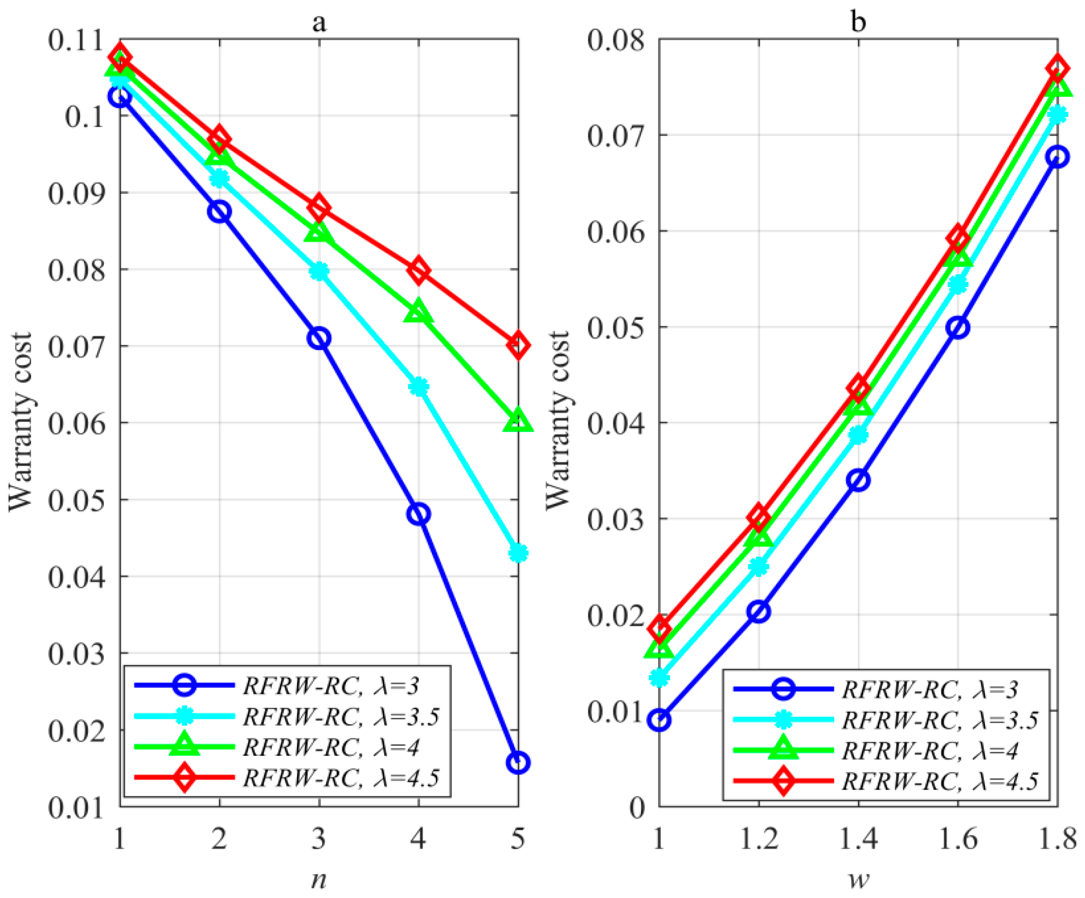
Figure 2 has been plotted to explore the properties of RFRW-RC.

Figure 2a with $w=2$ shows that the warranty cost of RFRW-RC decreases with respect to the warranty term $n$; the warranty cost of RFRW-RC increases with the failure rate $\lambda$. The increase of the warranty term $n$ enhances the manufacturer’s charge, which can reduce the manufacturer’s warranty cost. Therefore, the former case occurred. The former signals that the warranty cost of RFRW-RC is a decreasing function with respect to the warranty term $n$. This is different from 2DFRWF and 2DFRWL in Ref. [17], under which the warranty cost of each warranty model is an increasing function with the increase in the warranty term $n$. Figure 2b with $n=2$ shows that the warranty cost of RFRW-RC increases with the span time $w$; the warranty cost of RFRW-RC also increases with the failure rate $\lambda$. The increase in the span time $w$ enhances the manufacturer’s rebate that can increase the manufacturer’s warranty cost. Therefore, the first case occurred. In Figure 2, the cause that the failure rate $\lambda$ affects the warranty cost of RFRW-RC has been explained in Ref. [17], and here no longer present them.

Figure 3 explores the properties of RDFRW. Figure 3 shows that with the increase in $n$, the warranty cost of RDFRW increases while the warranty cost of RDFRW decreases with the increase in $\lambda$. The key cause of the former is that the increase in $n$ enlarges the warranty range and thus enhances the warranty cost of RDFRW. The key cause of the latter is that the increase in $\lambda$ shortens the working cycle, which shrinks the warranty range, and thus, the warranty cost of RDFRW is reduced. Therefore, all change laws drawn from Figure 3 hold true.

4.2. Exploration of the Properties of the Presented Random Maintenance Models

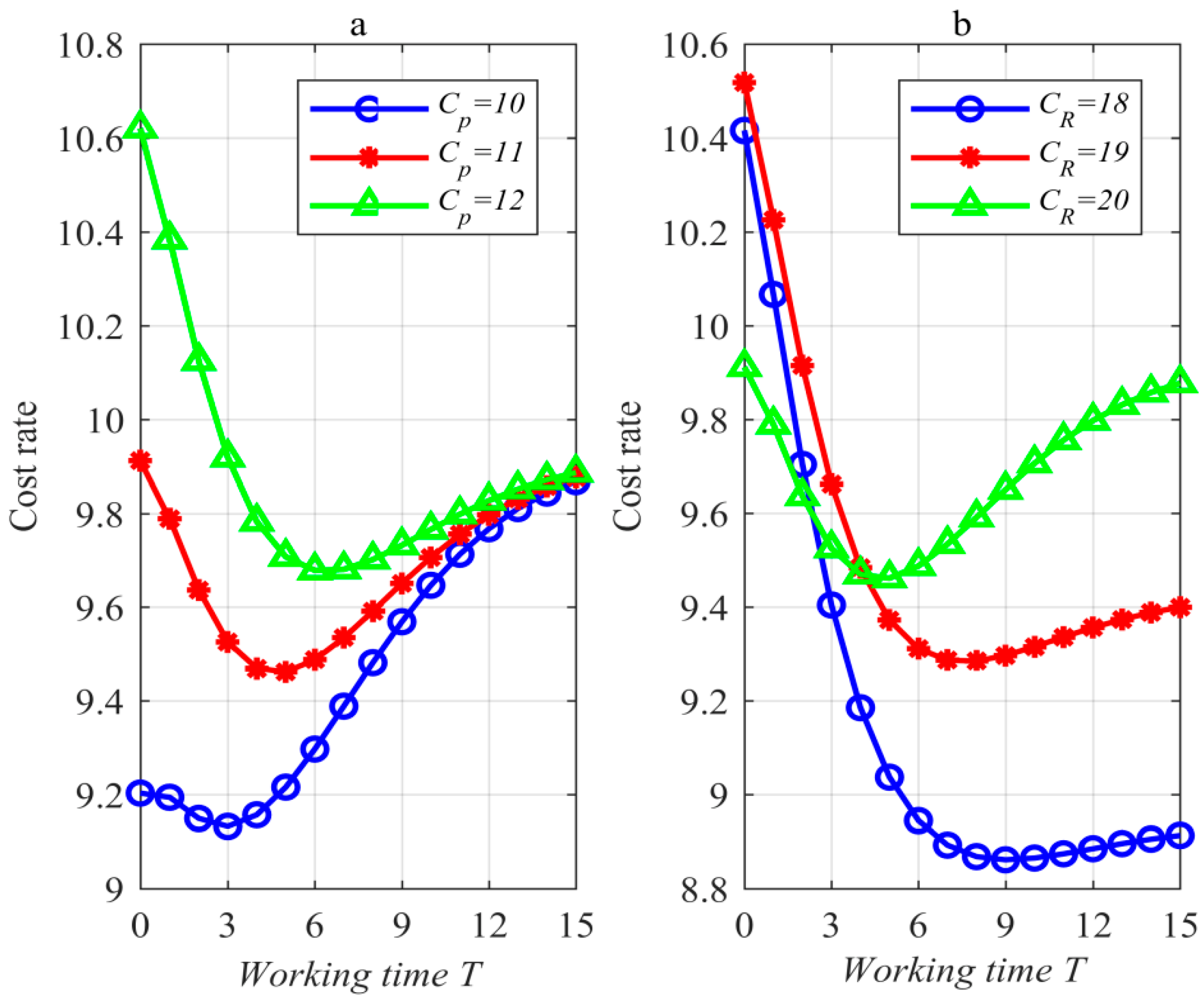
Figure 4 (where $w=2$, $\lambda =2$ and $n=2$) has been prepared to validate the existence and uniqueness of the optimal RHAR.

Figure 4 manifests that the optimal working time $T^{*}$ exists uniquely. Therefore, the optimal RHAR exists uniquely. Figure 4a, where $C_P=12$, shows that the increase in $C_P$ lengthens the optimal working time $T^{*}$ and enhances the optimal value $ECR(T^{*})$ of the cost rate. The cause of the former is that the increase in $C_P$ can enhance the expected total cost $LTC(T)$ during the life cycle.

Figure 4b, where $C_R=20$, shows that the increase in $C_R$ enhances the optimal value $ECR(T^{*})$ of the cost rate and reduces the optimal working time $T^{*}$. The cause of the former is similar to the cause of Figure 4a.

By comparing the above change laws, it is observed that a lower preventive replacement cost can reduce the optimal value of the cost rate while being unable to lengthen the system’s service period after warranty expiration; inversely, a lower corrective replacement cost can reduce the optimal value of the cost rate while lengthening the system’s service period after warranty expiration.

Table 2. The influence on the optimal RHAR of $w$ (where $n=2$, $C_R=20$ and $C_P=12$ ).

Optimal RHAR	$w=1$	$w=2$	$w=3$	$w=4$
$T^{*}$	1.29	1.28	1.26	1.18
$ECR(T^{*})$	9.6764	9.6394	9.5680	9.4677

presents how the time span $w$ affects the optimal RHAR. As presented in Table 2, the increase in $w$ shortens the optimal working time $T^{*}$ and decreases the optimal value $ECR(T^{*})$ of the cost rate. This signals that the increase in the time span $w$ can lower the optimal value $ECR(T^{*})$ of the cost rate and shorten the system’s service period after warranty expiration.

Table 3. The effect of $n$ on the optimal RHAR (where $w=0.5$, $C_R=20$ and $C_P=12$ ).

Optimal RHAR	$n=1$	$n=2$	$n=3$
$T^{*}$	1.96	1.03	0.04
$ECR(T^{*})$	11.1599	9.6773	8.0181

has been plotted to explore how the warranty term $n$ affects the optimal RHAR. Table 3 shows that the increase in $n$ shortens the optimal working time $T^{*}$ and decreases the optimal value $ECR(T^{*})$ of the cost rate, which are similar to Table 2. This change law means that the relationship between a longer warranty service period and a longer service period after warranty expiration is catching one and losing another.

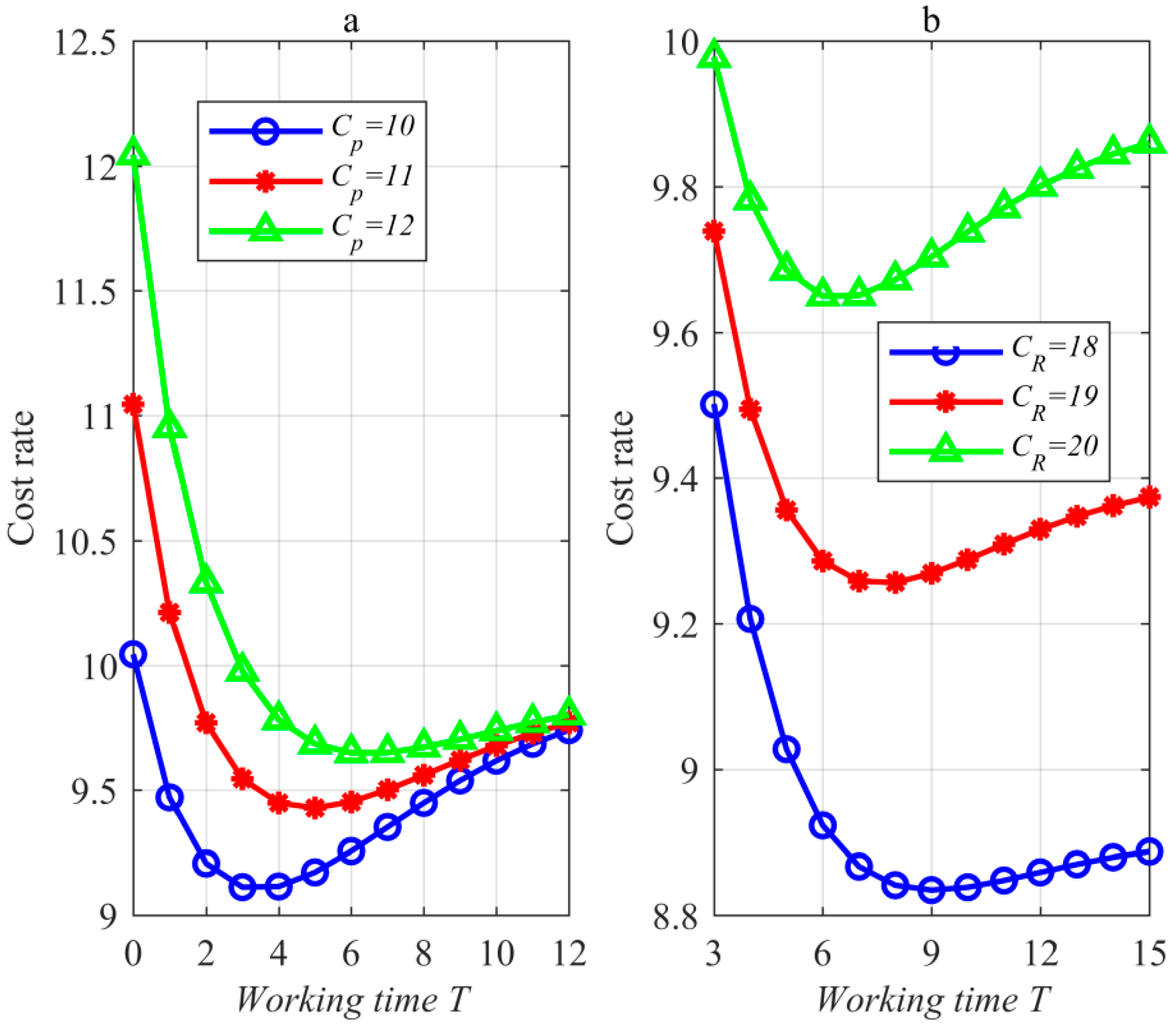
Figure 5 (where $w=2$, $\lambda =2$ and $n=2$) has been prepared to verify if the optimal CAR exists uniquely.

Figure 5 indicates that the optimal working time $T^{*}$ uniquely exists. Therefore, the optimal CAR exists uniquely. Figure 5a, where $C_P=12$, shows that the increase in $C_P$ lengthens the optimal working time $T^{*}$ and enhances the optimal value $ECR(T^{*})$ of the cost rate. Figure 5b, where $C_R=20$, shows that the increase in $C_R$ enhances the optimal value $ECR(T^{*})$ of the cost rate and reduces the optimal working time $T^{*}$. The above laws are similar to the changes in Figure 4, and therefore, the insights are similar to those of Figure 3. In Figure 5, the cause that the increase in $C_P$ and $C_R$ enhances the optimal value $ECR(T^{*})$ is similar to the cause of Figure 4.

Table 4. The effect of $n$ on the optimal AR (where $\lambda =2$, $C_R=20$ and $C_P=12$ ).

Optimal CAR	$n=1$	$n=2$	$n=3$
$T^{*}$	2.53	1.79	0.92
$ECR(T^{*})$	10.1289	8.8347	7.5431

explores how the warranty term $n$ affects the optimal CAR. As indicated in Table 4, the increase in $n$ shortens the optimal working time $T^{*}$ and decreases the optimal value $ECR(T^{*})$ of the cost rate. This is similar to Table 3. Such signals that the increase in the warranty term $n$ can lower the optimal value of the cost rate and shorten the system’s service period after warranty expiration. Therefore, similar to Table 3, this change law means that the relationship between a longer warranty service period and a longer service period after warranty expiration is catching one and losing another.

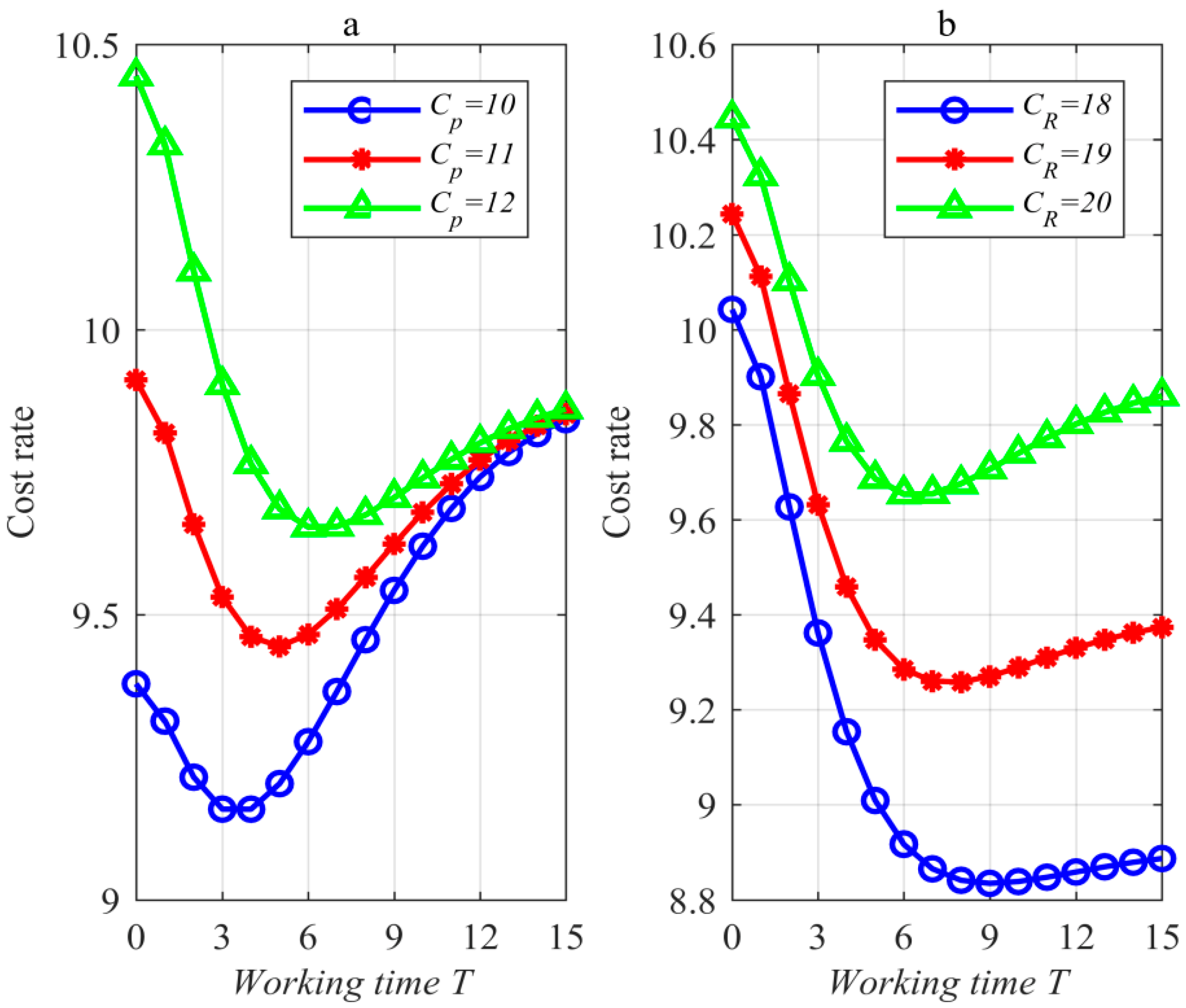
Figure 6 (where $w=2$, $\lambda =2$ and $n=2$) has been drawn to verify if the optimal RARL exists uniquely. Figure 6 shows that the optimal working time $T^{*}$ exists uniquely, which means that the optimal RARL exists uniquely. Figure 6a, where $C_P=12$, shows that the increase in $C_P$ lengthens the optimal working time $T^{*}$ and enhances the optimal value $ECR(T^{*})$ of the cost rate. Figure 6b, where $C_R=20$, shows that the increase in $C_R$ enhances the optimal value $ECR(T^{*})$ of the cost rate and reduces the optimal working time $T^{*}$. The above laws are similar to Figure 4 and Figure 5, and therefore, the explanations and insights are similar to those of Figure 4 and Figure 5.

Table 5. The effects of $n$ on the optimal RARL (where $\lambda =2$, $C_R=20$ and $C_P=12$ ).

Optimal RARL	$n=1$	$n=2$	$n=3$
$T^{*}$	2.24	1.3	0.59
$ECR(T^{*})$	10.6495	9.2572	7.8312

has been provided to explore how the warranty term $n$ affects the optimal RARL. Table 5 shows that the increase in $n$ shortens the optimal working time $T^{*}$ and decreases the optimal value $ECR(T^{*})$ of the cost rate. This is similar to Table 3 and Table 4. This signals that the increase in the warranty term $n$ can lower the optimal value of the cost rate and shorten the system’s service period after warranty expiration. Without exception, the insights are the same as those of Table 3 and Table 4.

Note: in this paper, three types of maintenance policies have been provided to ensure system reliability during the post-warranty stage and have been analyzed as well as validated in form of some key parameters in models. The selection of the maintenance policy is affected by many factors. Cost or/and time are two types of key measure to select a best maintenance policy. From the viewpoint of a cost or time measure, Refs. [] have presented a comparative method to select the best maintenance policy. In view of this, we have not presented the selection of the best maintenance policy; please consult the above literature for this.

5. Conclusions

By defining limited random working cycles, a rebate and a charge as warranty terms, this paper devises a novel warranty, which is named a random free repair warranty with rebate and charge (RFRW-RC). In such an RFRW-RC, the rebate is used to remove the manufacturer’s responsibility for continuing to ensure the system reliability, and the charge serves as a support where the manufacturer is responsible for continuing to ensure the system reliability. The warranty cost of RFRW-RC is derived and analyzed. By discussing terms of RFRW-RC, a special warranty model is presented, which is named the random discrete free repair warranty (RDFRW). For RDFRW, discrete data, i.e., limited random working cycles, are a unique warranty limitation, and minimal repairs are used to eliminate all failures. By simplifying the warranty cost of RFRW-RC, the warranty cost of RDFRW is obtained. Under RFRW-RC, the cases in which the system’s warranty expires can be classified into two types. The first type is that the system’s warranty expires at the completion of the limited random working cycles before a span time (i.e., warranty period), and the second type is that the system’s warranty expires at a span time after the completion of limited random working cycles. This means that RFRW-RC produces two different system ages. By differentiating system ages, a random hybrid maintenance policy is designed to ensure the system reliability after RFRW-RC expiration. This random hybrid maintenance policy is named the random hybrid age replacement (RHRA) policy, under which the random age replacement last (RARL) policy is used to ensure the reliability of the system through RFRW-RC at the completion of limited random working cycles before the end of a time span, and classic age replacement (CAR) is applied to ensure the reliability of the system through RFRW-RC at the completion of limited random working cycles after a span time. The objective function of RHRA is constructed, and the decision variable is optimized. By discussing parameter values, the objective function of RDFRW is presented. Finally, the presented models are illustrated from the viewpoint of numerical values. It is shown that the warranty cost of RFRW-RC does not necessarily increase with the increase in the number of random working cycles.

In recent years, pushed by the rapid development and wide application of advanced digital technologies, some countries are eagerly building nations, such as Germany and China. From the application’s perspective, all models presented in this paper can be applied in systems integrated with advanced digital technologies. In this paper, we confined problems to the system whose deterioration is characterized by a lifetime’s distribution function, and ignored the system whose deterioration is characterized by either a degradation process, a lifetime’s distribution function or both. Therefore, for the system whose deterioration is characterized by either a degradation process, a lifetime’s distribution function or both, some warranty models and post-warranty maintenance models can also be constructed. In addition, post-warranty maintenance models in this paper were constructed in the case where a warranty model considering ‘whichever occurs first’ is planned to ensure the system reliability during the warranty stage. In the case where a warranty model considering ‘whichever occurs last’ is planned to ensure system reliability during the warranty stage, constructing post-warranty maintenance models seldom appears, which is a future research direction.