Abstract
Driven by digital technologies, it is possible that high-tech equipment management personnel use monitored job cycles to ensure products’ operation and maintenance over their life cycle. By means of monitored job cycles, this paper designs two categories of random maintenance policies: a two-stage two-dimensional free repair warranty (2DFRW) policy and a random hybrid periodic replacement (RHPR) policy. The 2DFRW policy is performed to ensure the product’s operation and maintenance over the warranty stage. Under such a policy, a product is minimally repaired at each failure, and regions of the second-stage warranty are set to be diverse to remove all inequities produced by limitations of the first-stage warranty. The warranty cost of two-stage 2DFRW is built and discussed. The RHPR policy is modeled to ensure the product’s operation and maintenance over the post-warranty stage. Under this policy, depending on the final expiry of the two-stage 2DFRW, a bivariate random periodic replacement (BRPR) policy and a univariate random periodic replacement (URPR) policy are skillfully used to reduce the maintenance cost over the post-warranty stage and maximally extend the residual useful time of the product through the warranty. The expected cost rate over the product’s operation and maintenance cycle is derived on the basis of renewal rewarded theorem. The optimal RHPR policy is analyzed by minimizing the cost rate. The presented models are numerically analyzed to explore hidden characteristics.
MSC:
90B25
1. Introduction
From the perspective of the life cycle, the operation and maintenance of products can be divided into two categories: operation and maintenance during the warranty stage, and operation and maintenance during the post-warranty stage. In engineering practice, the operation and maintenance during the former stage are the sole responsibility of manufacturers, while the operation and maintenance during the latter stage are wholly the responsibility of users/consumers.
Warranty policies/models are frequently applied to ensure the product’s operation and maintenance during the warranty stage. Driven by the need for this practice, warranties have always been researched from the manufacturers’ perspective. The earliest and most extensive research on warranty modeled warranty by means of classic maintenance theory. For example, Ref. [1] integrated classic replacement policy into warranty theory and optimized a three-dimensional renewable combination warranty, and the other warranty models related to such have been proposed in Refs. [2,3,4]; by means of classic preventive maintenance (PM) policy, Ref. [5] designed a warranty contract considering PM, and similar warranty models considering PM have been proposed in Refs. [6,7,8]; by integrating classic minimal repair into warranty theory, Refs. [9,10] modeled free repair warranty models; and other more recent warranty developments can be found in Refs. [11,12,13].
Driven by the fact that stochastic degradation processes model the product’s deterioration tendency (see Refs. [14,15,16,17]). Refs. [18,19,20,21,22] proposed on-condition maintenance policies to ensure the operation and maintenance of the degradation product, and Refs. [23,24,25,26,27,28] modeled abort policies of degradation products. On the basis of on-condition maintenance policies, a novel type of warranty, i.e., the on-condition warranty, has received attention and been designed, as found in Refs. [29,30,31,32]. From the viewpoint of the technology background, this type of warranty is supported by modern sensor technology, Internet of Things, and communication technology, which are collectively known as digital technology. In other words, the improvement in the product’s operation and maintenance during the life cycle resulting from the wide application of digital technologies drives the development and application of on-condition warranties.
In addition to the above value, digital technologies can deliver products’ job cycles in real time to management personnel, which includes but is not limited to manufacturers and consumers/users. For example, management personnel/manufacturers of shared transport can receive all usage data of each form of shared transport by means of background servers and control centers that are integrated with digital technologies. Similarly, consumers/users of shared transport can check their usage data for shared transport by means of an application program (AP) in mobile devices integrated with digital technologies. Motivated by the aforementioned engineering practice and defining all job cycles as random variables, some scholars and researchers (see Refs. [33,34,35,36]) have proposed a type of random maintenance to ensure the product’s operation and maintenance. On the basis of these random maintenance theories, a type of novel warranty, called a ‘random warranty’, was designed in Refs. [37,38,39].
Similarly, digital technologies can help the above random warranties ensure the product’s operation and maintenance over the warranty stage. Pushed by the increasingly extensive and in-depth application of digital technologies, the above random warranties will be increasingly popular in the future. From the perspective of brand image, an improper warranty can trigger some warranty discrimination, which badly damages the brand reputation of manufacturers. In view of these factors, Ref. [40] used a partial refund to address the user’s unfairness triggered by the differences in warranty expiration. Therefore, in addition to a partial refund, providing an extended service to users is also one method that can be used to remove the user’s unfairness. However, under the framework of a random warranty, few extended services have been used to maintain warranty fairness.
Maintenance policies/models are regularly applied to ensure the product’s operation and maintenance during the post-warranty stage. Such a type of maintenance policy can be classified into classic, on-condition and random maintenance policies. Classic maintenance policy is modeled based on a distribution function of lifetime, which can be found in Refs. [41,42,43,44,45]. An on-condition maintenance policy (see Ref. [46]) is proposed by using a stochastic degradation process. The random maintenance policy is modeled by means of random maintenance theory in Refs. [33,34,35,36], which was presented in Refs. [47,48].
Similar to random warranty models, existing random maintenance policies to ensure the product’s operation and maintenance over the post-warranty stage will be increasingly popular in the future as digital technologies are applied extensively and rapidly in practice. However, existing research generally ignores the fact that past ages of products are not the same due to the differences in warranty expiries. From the viewpoint of reliability theory, when the past ages at warranty expiry are different, both OM (i.e., operation and maintenance) cost and residual useful time during the post-warranty stage are not the same. This signals that, according to the difference in the past ages, designing a flexible maintenance policy is one of methods that can be used to greatly reduce OM cost and use maximally residual useful time.
Based on the above, Ref. [38] combined a random and classic maintenance policy, and modeled a random maintenance policy to ensure the product’s OM over the post-warranty stage. One point worth emphasizing is that the classic maintenance policy in this random maintenance policy was devised based on calendar time rather than monitored job cycles. This fact means that it is difficult to ensure OM in real time. The key cause is that the real-time usage data of products are not easy to obtain precisely when digital technologies are not used. This indicates that, under the case where digital technology is realized, classic maintenance policies based on calendar time are no longer the best method to ensure OM in real time. Therefore, under the case of digital technology realization, replacing classic maintenance policies with a random maintenance policy is an ideal method to greatly reduce OM cost and maximally use residual useful time. To the best of our knowledge, this type of replacement policy has never been modeled to ensure the product’s OM over the post-warranty stage.
By integrating random job cycles into a product’s OM over the life cycle, in this study a manufacturer’s random warranty policy was designed in order to ensure the product’s OM over the warranty stage, and then a consumer’s random maintenance policy was devised in order to ensure the product’s OM over the post-warranty stage. The manufacturer’s random warranty is classified into two stages, wherein the second-stage warranty is used to remove the consumer’s unfairness triggered by the first-stage warranty. In addition, minimal repair in this warranty is used to remove each failure that occurs during the warranty period. Therefore, it is named a two-stage two-dimensional free repair warranty (2DFRW) policy. The consumer’s random maintenance policy is as follows: (1) Depending on the final expiry of the two-stage 2DFRW, a bivariate random periodic replacement (BRPR) policy and a univariate random periodic replacement (URPR) policy are performed; (2) the BRPR policy is applied to maximally use the residual useful time of the product through the warranty; and (3) the URPR policy, which can shrink the replacement region, is performed to greatly reduce the OM cost over the post-warranty stage. It is obvious that the random maintenance policy is a mixture of BRPR and URPR. Thus, it is named the random hybrid periodic replacement (RHPR) policy. The two-stage 2DFRW and RHPR are mathematically modeled and then numerically analyzed to explore hidden characteristics.
This paper is organized as follows. Section 2 presents the design of the two-stage 2DFRW model, and the related warranty cost and some special warranty models. In Section 3, the RHPR policy is modeled to ensure the product’s operation and maintenance over the post-warranty stage. The existence and uniqueness of the RHPR policy is summarized in Section 4. Section 5 explores the properties of the proposed models from the viewpoint of the numeric analysis. Section 6 concludes the paper.
2. Design of Random Warranty Policy
Similar to Refs. [38,47,48], the assumptions used are listed below: the product works for projects at job cycles and the job cycles of all projects are random job cycles; each random job cycle is subject to an identical distribution function , wherein its memory does not exist; the first failure time X is subject to the distribution function , whose failure rate function is r (u); and the time to repair or replacement is negligible.
2.1. Definition of Random Warranty
Let , , and be three warranty periods, where and ; let , , and be three discrete positive natural numbers, where . We divide the whole warranty into two stages: the first-stage warranty and the second-stage warranty. The first-stage warranty is used to warrant a new product, and the second-stage warranty is triggered when the first-stage warranty expires. The warranty region of the first-stage warranty is composed of the warranty period and the random job cycle completion. The warranty region of the second-stage warranty is composed of the warranty period and the random job cycle completion, or the warranty period and the random job cycle completion. Under these declarations, a two-stage 2DFRW is described as follows:
- The product is minimally repaired at each failure.
- The first-stage warranty expires at the warranty period w1 or the n1th random job cycle completion, whichever occurs first.
- If the product goes through the first-stage warranty at the n1th random job cycle completion, then such a product will be warranted by the second-stage warranty whose expiry occurs at the warranty period w2 or the n2th random job cycle completion, whichever occurs first.
- If the product goes through the first-stage warranty at w1, then such a product will be warranted by the second-stage warranty whose expiry occurs at the warranty period w3 or the n3th random job cycle completion, whichever occurs first.
Notes: ① Under the case of w2 > w3 and n2 > n3, the superficial area of region (0, n2] × (0, w2] is greater than the superficial area of region . This relationship implies that the second-stage warranty with region can remove the complaints of users whose first-stage warranty expires at the n1th random job cycle completion rather than at w1. ② Under the case where the second-stage warranty with region is triggered, the related warranty service period could be greater than w1. Therefore, the second-stage warranty with region is used to maintain the fairness of users whose first-stage warranty expires at w1 rather than at the n1th random job cycle completion.
When the n1th random job cycle is completed, the product’s working time is , which is a sum of n1 random job cycles, where . According to probability theory, the distribution function and reliability function of are and . When the product goes through the first-stage warranty at the n1th random job cycle completion, the product age is accurately obeying the distribution function , i.e.,
where .
When the n2th random job cycle completes before w2, the warranty service period produced by the second-stage warranty with the region is . Similarly, obeys the distribution function with the expression:
where s2 < w2 and is the distribution function of .
Heretofore, we have assumed that the distribution function G(y) of the random job cycles Yi has no memory. This signals that the remaining completion time after w1 for a random job cycle is still subject to G(y). Therefore, when the n3th random job cycle completes first, the warranty service period is produced by the second-stage warranty with region is . Similarly, is subject to the distribution function , i.e.,
where and is the distribution function of .
2.2. Cost Evaluation of Random Warranty
2.2.1. Cost Evaluation of the First-Stage Warranty
The two-stage 2DFRW requires that the product is minimally repaired at each failure. Let cm be the cost of minimal repair, which is named the unit repair cost. Then, the repair cost of the product whose first-stage warranty expires at can be computed as , and the repair cost of the product whose first-stage warranty expires at the n1th random job cycle completion can be computed as , where . Because the probabilities that the product goes through the first-stage warranty at w1 or the n1th random job cycle completion are and , the total repair cost of the first-stage warranty can be computed as:
2.2.2. Cost Evaluation of the Second-Stage Warranty
When the product goes through the first stage warranty at w1, then the second stage warranty with the region will be triggered to warrant such a product. For the product through the first-stage warranty at w1, its age is equal to w1, and its failure rate function at w1 is modeled as . Similar to the derivation process of Equation (4), for the product through the first-stage warranty at w1, the total repair cost of the second-stage warranty can be computed as:
By replacing w1, w3, s2, and n3 with , w2, s3, and n2, for the product through the first stage warranty at the n1th random job cycle completion, the total repair cost of the second stage warranty can be computed as:
Because the probabilities that the product goes through at w1 or the n1th random job cycle completion are and , the total repair cost WC2 of the second-stage warranty can be computed as:
2.2.3. Cost Evaluation of Two-Stage 2DFRW
By the definition of the two-stage 2DFRW, the warranty cost of the two-stage 2DFRW includes two section costs, the warranty cost of the first-stage warranty and the warranty cost of the second warranty. Therefore, by summing Equations (4) and (7), the warranty cost WC of the two-stage 2DFRW can be obtained as:
2.3. Simplification of Random Warranty
When w3 = w2 and n3 = n2, the warranty cost WC of the two-stage 2DFRW is rewritten as:
w3 = w2 and n3 = n2 indicate that two regions of the second-stage warranty are unified into the same region, which is expressed as . Therefore, this model is the warranty cost of the two-stage 2DFRW, wherein the warranty period w1 and the n1th random job cycle completion still constrain the first stage warranty, while the second stage warranty is constrained by the warranty period w2 and the n2th random job cycle completion rather than the warranty period w3 and the n3th random job cycle completion.
When w3 = w2 and n3 = n2 = ∞, the warranty cost WC of the two-stage 2DFRW is rewritten as:
w3 = w2 and n3 = n2 = ∞ indicate that two regions of the second-stage warranty are reduced to a common one-dimensional warranty period. In other words, when w3 = w2 and n3 = n2 = ∞, 2DFRW in the second-stage warranty is reduced to a classic FRW. Obviously, the first-stage warranty is a 2DFRW, while the second-stage warranty is a classic FRW. In view of this, the two-stage 2DFRW in Equation (10) is called a two-stage hybrid FRW (HFRW); thus, the warranty cost of Equation (10) is the cost of the two-stage HFRW.
When w3 = w2 = 0 and n3 = n2 = ∞, the warranty cost WC of the two-stage 2DFRW is rewritten as:
w3 = w2 = 0 and n3 = n2 = ∞ mean that the second-stage warranty is removed, and thus, the two-stage 2DFRW is reduced to 2DFRWF in Ref. [47]. Therefore, the warranty cost of (11) is the cost of the 2DFRWF.
3. Design of Random Maintenance Policy
From the reliability perspective, the replacement regions produced by maintenance policies to ensure the operation and maintenance of the product through the warranty have an apparent effect on the maintenance cost and residual useful time of the product through the warranty. If the replacement region produced by a random periodic replacement is greater, the residual useful time of the product through the warranty will be extended. However, if the replacement region produced by a random periodic replacement is smaller, then the maintenance cost of the product through the warranty will be reduced. These results imply that skillfully combining random periodic replacement policies is one method to reduce the maintenance cost of the product through the warranty and maximally use the residual useful time of the product through the warranty. Considering this, under the assumption that the two-stage 2DFRW ensures operation and maintenance over the warranty stage, this section presents a random maintenance policy to reduce the maintenance cost of the product through the warranty and maximally use the residual useful time of the product through the warranty.
3.1. Definition of Random Maintenance Policy
In Ref. [47], random periodic replacement first (RPRF) is considered one of the methods to ensure product reliability after the expiration of warranties. The replacement region of such an RPRF is composed of the first job cycle completion and a replacement time T. If the first job cycle completion is extended to the Mth random job cycle completion, then the replacement region will be extended. For convenience, we name RPRF with the Mth job cycle a bivariate random periodic replacement (BRPR) policy because there exist two decision variables (i.e., M and T); we name RPRF with the first job cycle completion a univariate random periodic replacement (URPR) policy because a decision variable (i.e., T) is considered to be just.
Next, by skillfully combining RPRF and URPR, we devise a random maintenance policy to ensure the product’s OM over the post-warranty stage, as shown below.
- If the final expiration of the two-stage 2DFRW occurs at the n2th or n3th random job cycle completion, then the product’s OM will be ensured by BRPR, under which the product is minimally repaired at each failure and is replaced at the Mth random job cycle completion or a working time T, whichever occurs first.
- If the final expiration of the two-stage 2DFRW occurs at w2 or w3, then the product’s OM will be ensured by URPR, under which the product is minimally repaired at each failure and is replaced at the first random job cycle completion or a working time T, whichever occurs first.
Obviously, such a random replacement policy is composed of BRPR and URPR. Therefore, we name it a random hybrid periodic replacement (RHPR) policy. If M = 1, then RHPR is simplified as URPR.
When the final expiration of the two-stage 2DFRW occurs at the n2th or n3th random job cycle completion, product ages are or . When the final expiration of the two-stage 2DFRW occurs at w2 or w3, product ages are or w1 + w3. Under the case where ‘whichever occurs first’ is used as a constraint, the product age is less than the product age , i.e., ; the product age is less than the product age w1 +w3, i.e., . The former inequality implies that when the warranty expires at the n2th random job cycle completion, the longer residual useful life of the product through warranty has not been used; and when the warranty expires at w2, the maintenance cost of the product through warranty will be greater due to the product age being greater. A similar principle holds for the latter inequality. The region produced by BRPR is greater than the region (0, 1] × (0, T] produced by URPR. This relationship signals that BRPR can greatly lengthen the residual useful life of the product through the warranty, and URPR can reduce the maintenance cost of the product through warranty. In other words, RHPR is one method to solve the problem that the residual useful life of the product through a warranty is reduced and the maintenance cost of the product through a warranty is reduced.
3.2. Objective Function Modeling of RHPR
In this paper, our main purpose is to design random policies to ensure the product’s operation and maintenance over the life cycle. In the last section, a random warranty policy was designed to ensure the product’s operation and maintenance over the warranty stage. From reliability theory, the RHPR to ensure the product’s operation and maintenance over the post-warranty stage is affected by the product warranty, which was pointed out previously. This signals that the product warranty must be considered in the process of modeling the objective function of RHPR. In view of this, we define the operation and maintenance cycle of products as a time span consisting of the time span (i.e., a warranty service period) produced by the product warranty and the time span produced by the RHPR. On the basis of such an operation and maintenance cycle, objective function modeling of RHPR is presented below.
3.2.1. Total Cost Derivation over the Operation and Maintenance Cycle
When the first-stage warranty expires at the n1th random job cycle completion, the product age is equal to . For such a product, when its second-stage warranty expires at the n2th random job cycle completion, its age is equal to . According to reliability theory, the failure rate function at is given by . Under the case where BRPR is used to ensure the OM of the product through the two-stage 2DFRW at the n2th random job cycle completion, the total repair cost of BRPR is represented by:
where cf is a failure cost and is the reliability function of the working time resulting from the Mth random job cycle completion.
Because and obey the respective distribution functions and , the total repair cost can be rewritten as:
For such a product, when the second-stage warranty expires at w2, its age is equal to . In this case, the failure rate function at is given by . Under the case where URPR is used to ensure the OM of the product through the two-stage 2DFRW at w2, the total repair cost of URPR is represented by:
By means of , the total repair cost can be rewritten as:
The probability that the product goes through the second-stage warranty at the n2th random job cycle completion is given by ; the probability that the product goes through the second-stage warranty at w2 is given by . Therefore, the expectation of the total repair cost after the second-stage warranty with the warranty region expiry is given by:
When the first-stage warranty expires at w1, the product age is equal to w1. For such a product, when the second-stage warranty expires at the n3th random job cycle completion, its age is equal to . Similarly, the failure rate function at is given by . When the BRPR is used to ensure the OM of the product through the two-stage 2DFRW at the n3th random job cycle completion, the total repair cost of the BRPR is represented by:
Because obeys the distribution function , the total repair cost can be rewritten as:
The past age of the product through two-stage 2DFRW at w3 is equal to w1 + w3. Similarly, the failure rate function at w1 + w3 is given by . When URPR is used to ensure the OM of the product through the two-stage 2DFRW at w3, the total repair cost of URPR is represented by:
The probability that the product goes through the second-stage warranty at the n3th random job cycle completion is given by ; the probability that the product goes through the second-stage warranty at w3 is given by . Therefore, the expectation of the total repair cost after the second-stage warranty with the warranty region expiry is given by:
The probability that the product goes through the first-stage warranty at the n1th random job cycle completion is given by ; the probability that the product goes through the first-stage warranty at w1 is given by . Therefore, the expectation of the total repair cost after the two-stage 2DFRW expiry is given by:
According to the definition of the operation and maintenance cycle, the total cost over the operation and maintenance cycle is derived as:
where: , which is the total cost produced by the two-stage 2DFRW; ; and is a replacement cost.
3.2.2. Length Construction of the Operation and Maintenance Cycle
According to the definition of the operation and maintenance cycle, the operation and maintenance cycle includes two time spans. The first time span is produced by the two-stage 2DFRW, and the second time span is produced by RHPR. In this subsection, the length of the operation and maintenance cycle is derived from the consumer perspective, as shown below.
When the product goes through the first-stage warranty at the n1th random job cycle completion, the product’s warranty service period is equal to , where ; when the product goes through the first-stage warranty at w1, the product’s warranty service period is equal to w1. Because the probabilities that the above two cases occur are and , the warranty service period produced by the first-stage warranty is modeled as:
where obeys the distribution function .
When the product goes through the second-stage warranty at the n2th random job cycle completion, the warranty service period of the second-stage warranty with warranty region is equal to , where ; when the product goes through the first-stage warranty at w2, the warranty service period of the second-stage warranty with warranty region is equal to w2. Because the probabilities that the above two cases occur are and , the warranty service period of the second-stage warranty with the warranty region is modeled as:
Similarly, the warranty service period of the second-stage warranty with the warranty region is modeled as:
Since the probability that the product goes through the first-stage warranty at the n1th random job cycle completion is given by and the probability that the product goes through the second-stage warranty at w3 is given by , the time span produced by the two-stage 2DFRW is derived as:
When URPR ensures the OM of the product through the second stage warranty at the n2th or n3th random job cycle completion, the time span produced by BRPR is given by:
where with and is the distribution function of the working time resulting from the Mth random job cycle completion.
Similar to the derivation of Equation (27), when URPR ensures the OM of the product through the second stage warranty at the w2 or w3, the time span produced by URPR is given by:
The probability that the product first goes through the warranty at the n1th random job cycle completion and then goes through the second stage warranty at the n2 thrandom job cycle completion or w2 is given by or . The probability that the product first goes through the warranty at w1 and then goes through the second-stage warranty at the n3th random job cycle completion or w3 is given by or . Therefore, when RHPR ensures the OM of the product through the two-stage 2DFRW, the time span produced by RHPR is given by:
According to the definition of the operation and maintenance cycle, the length of the operation and maintenance cycle is constructed as:
3.2.3. Objective Function Model of RHPR
The length of the operation and maintenance cycle and the total cost over the operation and maintenance cycle are presented in Equations (30) and (22), respectively. Letting and , by the renewal rewarded theorem in Ref. [49], the expected cost rate ECR(M, T) can be modeled as:
3.3. Simplification of RHPR
When , the expected cost rate model in Equation (31) is reduced to:
where: and .
reduces URPR to a classic random periodic replacement policy. This means that the RHPR is revised as a hybrid periodic replacement (HPR) policy, which is a mixture of BRPR and classic random periodic replacement (CRPR) policy. Therefore, the model in Equation (32) is an expected cost rate model, wherein the two-stage 2DFRW in Section 2.1, and HPR consisting of BRPR and CRPR, are successively used to ensure the product’s OM over the post-warranty stage.
When and , the expected cost rate model in Equation (31) is reduced to:
where: and .
As given in Equation (9), and reduce the two-stage 2DFRW to a two-stage 2DFRW where the warranty period and the random job cycle completion are still limitations of the first-stage warranty, while the second-stage warranty is composed of the warranty period and the random job cycle completion. In view of these, the model in Equation (33) is an expected cost rate model, wherein the two-stage 2DFRW in Equation (9) and RHPR are successively used to ensure the product’s OM over the operation and maintenance cycle.
When , and , the expected cost rate model in Equation (31) is reduced to:
where: and .
It has been pointed out that M = 1 means that RHPR is simplified as URPR. Therefore, the model in Equation (34) is an expected cost rate model, wherein the two-stage 2DFRW in Equation (9) and URPR are successively applied to ensure the product’s OM over the operation and maintenance cycle.
When , and , the expected cost rate model in Equation (31) is reduced to:
where: .
As given above, and simplify the two-stage 2DFRW as a two-stage HFRW, wherein the warranty period and the random job cycle completion limit the first-stage warranty, while the second-stage warranty only includes a warranty limitation, i.e., the warranty period . The model in Equation (35) is an expected cost rate model, wherein the two-stage HFRW in Equation (10) and URPR is successively applied to ensure the product’s OM over the operation and maintenance cycle.
When and , the expected cost rate model in Equation (31) is reduced to:
As given above, and simplify the two-stage 2DFRW as a 2DFRWF in Ref. [47], wherein the warranty period and the random job cycle completion are two warranty limitations and ‘whichever occurs first’ is used. In addition, M = 1 means that RHPR is simplified as URPR. Therefore, the model in Equation (36) is an expected cost rate model, wherein 2DFRWF and URPR are successively utilized to ensure the product’s OM over the operation and maintenance cycle.
4. Optimization of Decision Variables
In this section, the optimal RHPR that is expressed as optimal solutions M* and T* is analyzed by minimizing in Equation (31).
Considering that the expressions of and are undecided, it is intractable to obtain the optimal analytical solutions. By means of a two-stage optimization method, we summarize the existence and uniqueness of optimal solutions, as shown below.
By means of the inequality ECR (M + 1, T) – ECR (M, T) ≥ 0 for a given T, the optimum solution M* that minimizes ECR (M, T) in Equation (31) can be summarized as Theorem 1 below.
Theorem 1.
For T ∈ [0, +∞), the following descriptions can be obtained. If Δ(M) increases monotonically to +∞ with respect to M, then an optimal solution M* exists uniquely and satisfies bothand, where.
By differentiating ECR (M, T) with respect to T, the derivative (see Appendix A) of the expected cost rate ECR (M, T) can be obtained. Let be the numerator of ; then, can be presented by:
Obviously, when , one expression is obtained as:
Let be zero; then, one expression can be obtained as:
Obviously, the left-hand side of Equation (37) is equal to the right-hand side of Equation (31).
Let be equal to the right-hand side of Equation (37), i.e.,
Then, the optimal solution T* minimizing ECR (T) in (31) can be summarized as Theorem 2 below.
Theorem 2.
For M = 1, 2, …, the following results can be obtained.
- ➀
- When, the optimal solution T* can be described as
- Ifincreases monotonically to +∞ with respect to T*, the optimal solution T* exists uniquely and satisfies T* = 0, and the minimal cost rateis measured by means of ρ(0);
- Ifdecreases monotonically towith respect to, the optimal solutionexists uniquely and satisfies, and the minimal cost rateis measured by means of;
- Ifis nonmonotonic with respect toand if there is more than one root for the equation, at least an optimal solutionexists and satisfies, and the minimal cost rateis measured by means of.
- ➁
- When, the optimal solutioncan be described as
- Ifincreases monotonically towith respect to, a finite optimal solutionexists uniquely and satisfies, and the minimal cost rateis measured by means of;
- Ifis nonmonotonic with respect toand if, at least an optimal solutionexists and satisfies, and the minimal cost rateis measured by means of;
- Ifdecreases monotonically towith respect to, the optimal solutionexists uniquely and satisfies, and the minimal cost rateis measured by means of.
Models in (32)–(36) can be similarly analyzed, and the related process is no longer presented here.
5. Numerical Examples
In this paper, a two-stage 2DFRW and RHPR are modeled to ensure the product’s operation and maintenance over the life cycle. Although mathematic models related to them have been constructed by means of probability theory, their characteristics are difficult to obtain from the viewpoint of the analysis. To explore their characteristics, we perform the following numerical analysis.
From the viewpoint of reliability theory, the failure rate function modeling the product’s failure tendency monotonically increases with working time for most engineering products. Thus, it is assumed that the failure rate function can be depicted as a power function , wherein . The second assumption is that the failure rate function of all random job cycles is a nonnegative constant λ. Some parameters are assigned below: , , and ; and other parameters are assigned wherever applied.
5.1. Illustration of the Two-Stage 2DFRW
To explore how , , and alter the warranty cost of the two-stage 2DRFW, Figure 1 is presented under the case of , , , and .
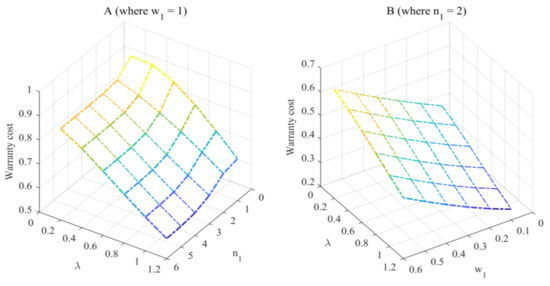
Figure 1.
How n1, w1, and λ affect the two-stage 2DRFW.
Figure 1A shows that the increase in can lower the warranty cost of the two-stage 2DFRW, and the increase in is also able to lower the warranty cost of the two-stage 2DFRW. The former change implies that the increase in the limitation of the first-stage warranty cannot enhance the warranty cost of the two-stage 2DFRW, which is not the same as the case of 2DFRWF in Ref. [47]. The main cause of the latter case is listed as follows: the increase in shortens the mean value of random job cycles, which reduces the warranty region of the first-stage warranty.
From Figure 1B, one discovery is that the effect of on the warranty cost of the two-stage 2DFRW is the same as the case of Figure 1A, while the increase in the limitation of the first-stage warranty enhances the warranty cost of the two-stage 2DFRW. The former case can be explained by the cause mentioned above. The latter case occurs because the increase in the limitation extends the warranty region of the first-stage warranty.
Under the case of , , and , Figure 2 is presented to explore how , , and alter the warranty cost of the two-stage 2DRFW.
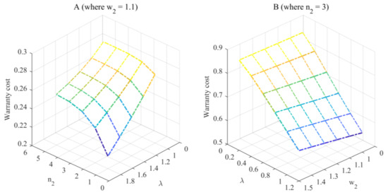
Figure 2.
How n2, w2, and λ affect the two-stage 2DRFW.
Figure 2A shows that the increase in makes the warranty cost of the two-stage 2DFRW a constant value, which is calculated by means of:
and the increase in is able to lower the warranty cost of the two-stage 2DFRW, which is the same as that of Figure 1. The former is because the increase in the limitation extends the warranty region of the second-stage warranty; the explanation of the latter is the same as the explanation in Figure 1A. From Figure 2B, one finds that the effect of on the warranty cost of the two-stage 2DFRW is the same as the case of Figure 2A, while the increase in the limitation of the second-stage warranty enhances the warranty cost of the two-stage 2DFRW. The former case can be explained by the explanation mentioned in Figure 1A. The latter case is because the increase in the limitation can enlarge the warranty region of the second-stage warranty.
By means of , , , , and , Figure 3 is plotted to explore how , , and affect the warranty cost of the two-stage 2DRFW. From Figure 3A, one finds that the increase in makes the warranty cost of the two-stage 2DFRW increase to a constant value, which can be measured by:
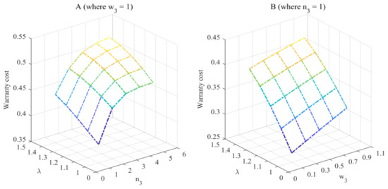
Figure 3.
How n3, w3, and λ affect the two-stage 2DRFW.
Figure 3B shows that the increase in the limitation of the second-stage warranty enhances the warranty cost of the two-stage 2DFRW. The above two cases can be explained by the fact that the increase in the limitation of the second stage warranty is able to extend the warranty region of the two-stage 2DFRW.
5.2. Illustration of RHPR
To validate the effectiveness of the designed RHPR, Figure 4 is drawn under the case of , , , , , , and . From Figure 4, we find that the value of the expected cost rate is minimal when . This signals that the designed RHPR is effective.
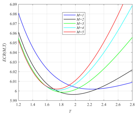
Figure 4.
The effectiveness validation of RHPR.
Under the case of , , , , , and (in Figure 5A) or (in Figure 5B), Figure 5 shows the effect of the first-stage warranty on the optimal RHPR.
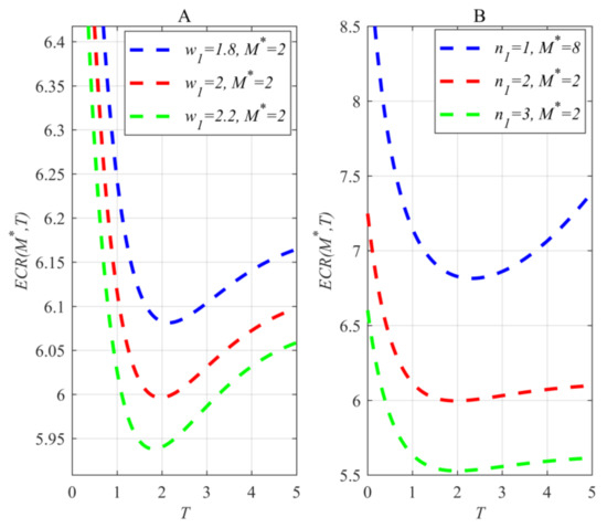
Figure 5.
The effect of n3 and w3 on the optimal RHPR.
Figure 5 shows that the increase in limitations of the first-stage warranty is able to reduce the minimal cost rate and shorten the optimal replacement time. This signals that obtaining a greater warranty region and obtaining a longer replacement time always address one thing and lose another.
Under the case of , , , , , and (in Figure 6A) or (in Figure 6B), Figure 6 is made to display the effect of and on the optimal RHPR. Figure 6A shows that the increase in the limitation can reduce the minimal cost rate and shorten the optimal replacement time. This signals that obtaining a greater warranty region and obtaining a longer replacement time always address one thing and lose another. Figure 6B shows that the increase in the limitation can enhance the minimal cost rate and prolong the optimal replacement time. This signals that the user can obtain a longer replacement time at a greater cost rate when the limitation is greater.
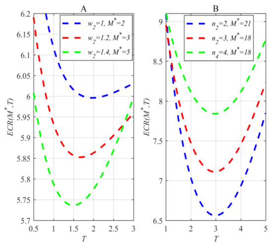
Figure 6.
The effect of n2 and w2 on the optimal RHPR.
Under the case of , , , , and (in Figure 7A) or (in Figure 7B), Figure 7 shows how and influence the optimal RHPR.
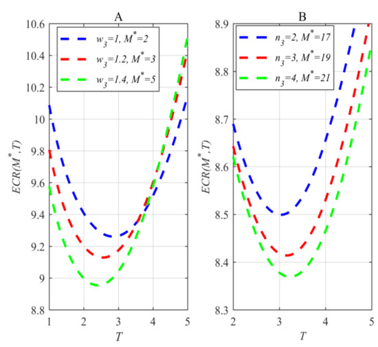
Figure 7.
The effect of n3 and w3 on the optimal RHPR.
Figure 7A shows that the increase in the limitation can lower the minimal cost rate and shorten the optimal replacement time. This signals that for users, just one occurs between the greater warranty region and longer replacement time. Figure 7B shows that the increase in the limitation is able to reduce the minimal cost rate and prolong the optimal replacement time. This signals that for users, the user can obtain a greater warranty region and a longer replacement time when the limitation is greater.
5.3. Illustration of RHPR Performance
By replacing classic maintenance policy with a random maintenance policy, this paper modeled the RHPR to ensure the product’s OM over the post-warranty period. In this subsection, RHPR performance is illustrated from a numerical perspective, as shown below.
The objective function model of RHPR is presented in Equation (31). By discussing the parameters in Equation (31), we obtained an objective function model of HPR, which was presented in Equation (32). Let and be values of numerator and , respectively; let and be values of denominator and , respectively. Then, and are computed by replacing M and T with optimal numerical solution and , which are obtained by minimizing ; and are computed by replacing M and T with optimal numerical solution and , which are obtained by minimizing . Under the case where and are multiplicative, we can judge the superiorities of RHPR and HPR by comparing the respective total costs, which are and .
By means of the above, Table 1 is obtained under the case of , , , , , and .

Table 1.
Performance comparison.
Table 1 shows that the total cost of RHPR is lower than the total cost of HPR. This relationship indicates that RHPR is superior to HPR. In other words, replacing classic maintenance policy with a random maintenance policy can lower the maintenance cost during the post-warranty stage or obtain a longer post-warranty period at a lower cost. In addition, we can also judge the superiorities of RHPR and HPR by comparing the respective cycle lengths, which was used in Ref. [47]. Regardless of the method used to compare performance, the results obtained are always the same.
6. Conclusions
Against a background in which digital technologies are being applied to improve product management, this paper proposes a manufacturer’s random warranty and consumer’s random maintenance policy in order to successively ensure the product’s operation and maintenance over its life cycle.
Differing from traditional random warranties under which a refund was used to maintain warranty fairness, in this paper, the extended service is used to maintain warranty fairness. The warranty cost of the presented random warranty is derived from the viewpoint of probability theory.
Under the case where the random warranty is presented in this paper, a consumer’s random maintenance policy is modeled by mixing two maintenance policies. The first maintenance policy is a bivariate random periodic replacement (BRPR) policy that can enlarge the replacement region to maximally use the residual useful time of the product through the warranty; the second maintenance policy is a univariate random periodic replacement (URPR) policy that can shrink the replacement region to reduce the maintenance cost of the product through the warranty. The cost rate of the consumer’s random maintenance policy is derived based on the renewal rewarded theorem and then is simplified to present some special maintenance policies to ensure the product’s operation and maintenance (OM) over the post-warranty stage. Two decision variables are optimized by minimizing the objective function. By means of numerical experiments, the proposed models are illustrated to explore hidden characteristics.
Although the extended service of this paper is one method to ensure the warranty fairness, investigation of the collective application of extended service and a refund to ensure warranty fairness seldom appears in the published works. Therefore, designing a random warranty with an extended service and a refund is a novel topic. By means of random job cycles, the design of a random cooperation contract between a product consumer and third-party maintenance service provider is also an interesting topic. These topics are being studied by authors.
Author Contributions
Conceptualization, L.S. and L.W.; methodology, L.S.; software, Y.D.; validation, Y.D.; formal analysis, L.S. and X.Y.; investigation, L.S., L.W. and X.Y.; resources, Y.D.; data curation, X.Y.; writing—original draft preparation, L.S.; writing—review and editing, L.S.; visualization, L.W.; supervision, L.W.; project administration, X.Y.; funding acquisition, Y.D. All authors have read and agreed to the published version of the manuscript.
Funding
This study is supported by the Characteristic Innovation Projects of Colleges and Universities in Guangdong Province (No. 2021WTSCX081), the Base and Basic Applied Study of Guangdong Province (No. 2020A1515011360), the National Natural Science Foundation of China (Nos. 71871181, 72161025, 72271169).
Institutional Review Board Statement
Not applicable.
Informed Consent Statement
Not applicable.
Data Availability Statement
The authors confirm that the data supporting the findings of this study are available within the article.
Conflicts of Interest
The authors declare no conflict of interest.
Appendix A
The derivative of the expected cost rate is represented by:
References
- Qiao, P.; Shen, J.; Zhang, F.; Ma, Y. Optimal warranty policy for repairable products with a three-dimensional renewable combination warranty. Comput. Ind. Eng. 2022, 168, 108056. [Google Scholar] [CrossRef]
- Wang, X.; He, K.; He, Z.; Li, L.; Xie, M. Cost analysis of a piece-wise renewing free replacement warranty policy. Comput. Ind. Eng. 2019, 135, 1047–1062. [Google Scholar] [CrossRef]
- Liu, B.; Wu, J.; Xie, M. Cost analysis for multi-component system with failure interaction under renewing free-replacement warranty. Eur. J. Oper. Res. 2015, 243, 874–882. [Google Scholar] [CrossRef]
- Rao, B.M. Cumulative free replacement warranty with phase type lifetime distributions. Comput. Ind. Eng. 2021, 162, 107771. [Google Scholar] [CrossRef]
- Iskandar, B.P.; Sa’idah, N.F.; Pasaribu, U.S.; Cakravastia, A.; Husniah, H. Warranty and maintenance service contracts for repairable products. Alex. Eng. J. 2022, 61, 10819–10835. [Google Scholar] [CrossRef]
- Hashemi, M.; Asadi, M.; Tavangar, M. Optimal maintenance strategies for coherent systems: A warranty dependent approach. Reliab. Eng. Syst. Saf. 2022, 217, 108027. [Google Scholar] [CrossRef]
- He, Z.; Wang, D.; He, S.; Zhang, Y.; Dai, A. Two-dimensional extended warranty strategy including maintenance level and purchase time: A win-win perspective. Comput. Ind. Eng. 2020, 141, 106294. [Google Scholar] [CrossRef]
- Peng, S.; Jiang, W.; Wei, L.; Wang, X.L. A new cost-sharing preventive maintenance program under two-dimensional warranty. Int. J. Prod. Econ. 2022, 233, 107974. [Google Scholar] [CrossRef]
- Wang, L.; Pei, Z.; Zhu, H.; Liu, B. Optimising extended warranty policies following the two-dimensional warranty with repair time threshold. Eksploat. I Niezawodn. Maint. Reliab. 2018, 20, 523–530. [Google Scholar] [CrossRef]
- Hooti, F.; Ahmadi, J.; Longobardi, M. Optimal extended warranty length with limited number of repairs in the warranty period. Reliab. Eng. Syst. Saf. 2020, 203, 107111. [Google Scholar] [CrossRef]
- Gupta, S.K.; Mukhopadhyay, I.; Chatterjee, A. Two-dimensional extended warranty length design from incomplete warranty data based on a new price curve considering different maintenance policies. Comput. Ind. Eng. 2022, 170, 108323. [Google Scholar] [CrossRef]
- Wang, X.; Xie, W.; Ye, Z.S.; Tang, L. Aggregate discounted warranty cost forecasting considering the failed-but-not-reported events. Reliab. Eng. Syst. Saf. 2017, 168, 355–364. [Google Scholar] [CrossRef]
- Wang, X.; Ye, Z.S. Design of customized two-dimensional extended warranties considering use rate and heterogeneity. IISE Trans. 2020, 53, 341–351. [Google Scholar] [CrossRef]
- Ye, Z.S.; Xie, M. Stochastic modelling and analysis of degradation for highly reliable products. Appl. Stoch. Models Bus. Ind. 2015, 31, 16–32. [Google Scholar] [CrossRef]
- Yan, B.; Ma, X.; Yang, L.; Wang, H.; Wu, T. A novel degradation-rate-volatility related effect Wiener process model with its extension to accelerated ageing data analysis. Reliab. Eng. Syst. Saf. 2020, 204, 107138. [Google Scholar] [CrossRef]
- Wang, H.; Zhao, Y.; Ma, X.; Yang, L. Equivalence analysis of accelerated degradation mechanism based on stochastic degradation models. Qual. Reliab. Eng. Int. 2017, 33, 2281–2294. [Google Scholar] [CrossRef]
- Wang, J.; Qiu, Q.; Wang, H.; Lin, C. Optimal condition-based preventive maintenance policy for balanced systems. Reliab. Eng. Syst. Saf. 2021, 211, 107606. [Google Scholar] [CrossRef]
- Liu, B.; Pandey, M.D.; Wang, X.; Zhao, X. A finite-horizon condition-based maintenance policy for a two-unit system with dependent degradation processes. Eur. J. Oper. Res. 2021, 295, 705–717. [Google Scholar] [CrossRef]
- Li, H.; Zhu, W.; Dieulle, L.; Deloux, E. Condition-based maintenance strategies for stochastically dependent systems using Nested Lévy copulas. Reliab. Eng. Syst. Saf. 2022, 217, 108038. [Google Scholar] [CrossRef]
- Yang, L.; Ma, X.; Zhao, Y. A condition-based maintenance model for a three-state system subject to degradation and environmental shocks. Comput. Ind. Eng. 2017, 105, 210–222. [Google Scholar] [CrossRef]
- Yang, L.; Ma, X.; Zhao, Y. A condition-based maintenance model based on a two-stage degradation process. In Proceedings of the 10th International Conference on Mathematical Methods in Reliability (MMR 2017), Grenoble, France, 3–6 July 2017; ISTP: Buraydah, Saudi Arabia, 2017. [Google Scholar]
- Wang, J.; Qiu, Q.; Wang, H. Joint optimization of condition-based and age-based replacement policy and inventory policy for a two-unit series system. Reliab. Eng. Syst. Saf. 2021, 205, 107251. [Google Scholar] [CrossRef]
- Qiu, Q.; Cui, L. Gamma process based optimal mission abort policy. Reliab. Eng. Syst. Saf. 2019, 190, 106496. [Google Scholar] [CrossRef]
- Zhao, X.; Fan, Y.; Qiu, Q.; Chen, K. Multi-criteria mission abort policy for systems subject to two-stage degradation process. Eur. J. Oper. Res. 2021, 295, 233–245. [Google Scholar] [CrossRef]
- Zhao, X.; Sun, J.; Qiu, Q.; Chen, K. Optimal inspection and mission abort policies for systems subject to degradation. Eur. J. Oper. Res. 2021, 292, 610–621. [Google Scholar] [CrossRef]
- Qiu, Q.; Maillart, L.M.; Prokopyev, O.A.; Cui, L. Optimal Condition-Based Mission Abort Decisions. IEEE Trans. Reliab. 2022, 292, 610–621. [Google Scholar] [CrossRef]
- Zhao, X.; Chai, X.; Sun, J.; Qiu, Q. Joint optimization of mission abort and protective device selection policies for multistate systems. Risk Anal. 2022, 13869. [Google Scholar] [CrossRef] [PubMed]
- Yang, L.; Chen, Y.; Qiu, Q.; Wang, J. Risk control of mission-critical systems: Abort decision-makings integrating health and age conditions. IEEE Trans. Ind. Inf. 2022, 18, 6887–6894. [Google Scholar] [CrossRef]
- Li, T.; He, S.; Zhao, X. Optimal warranty policy design for deteriorating systems with random failure threshold. Reliab. Eng. Syst. Saf. 2022, 218, 108142. [Google Scholar] [CrossRef]
- Cha, J.H.; Finkelstein, M.; Levitin, G. Optimal warranty policy with inspection for heterogeneous, stochastically degrading items. Eur. J. Oper. Res. 2021, 289, 1142–1152. [Google Scholar] [CrossRef]
- Zhang, N.; Fouladirad, M.; Barros, A. Evaluation of the warranty cost of a product with type III stochastic dependence between components. Appl. Math. Model. 2018, 59, 39–53. [Google Scholar] [CrossRef]
- Zhang, N.; Fouladirad, M.; Barros, A. Warranty analysis of a two-component system with type I stochastic dependence. Proc. Inst. Mech. Eng. Part O J. Risk Reliab. 2018, 232, 274–283. [Google Scholar] [CrossRef]
- Sheu, S.H.; Liu, T.H.; Zhang, Z.G. Extended optimal preventive replacement policies with random working cycle. Reliab. Eng. Syst. Saf. 2019, 188, 398–415. [Google Scholar] [CrossRef]
- Nakagawa, T. Random Maintenance Policies; Springer: London, UK, 2014. [Google Scholar]
- Zhao, X.; Nakagawa, T.; Zuo, M.J. Optimal replacement last with continuous and discrete policies. IEEE Trans. Reliab. 2014, 63, 868–880. [Google Scholar] [CrossRef]
- Zhao, X.; Nakagawa, T. Optimization problems of replacement first or last in reliability theory. Eur. J. Oper. Res. 2012, 223, 141–149. [Google Scholar] [CrossRef]
- Shang, L.; Zou, A.; Qiu, Q.; Du, Y. A random maintenance last model with preventive maintenance for the product under a random warranty. Eksploat. I Niezawodn. Maint. Reliab. 2022, 24, 544–553. [Google Scholar] [CrossRef]
- Shang, L.; Yu, X.; Du, Y.; Zou, A.; Qiu, Q. An Optimal Random Hybrid Maintenance Policy of Systems under a Warranty with Rebate and Charge. Mathematics 2022, 10, 3229. [Google Scholar] [CrossRef]
- Du, Y.; Shang, L.; Qiu, Q.; Yang, L. Optimum Post-Warranty Maintenance Policies for Products with Random Working Cycles. Mathematics 2022, 10, 1694. [Google Scholar] [CrossRef]
- Shang, L.; Du, Y.; Wu, C.; Ma, C. A Bivariate Optimal Random Replacement Model for the Warranted Product with Job Cycles. Mathematics 2022, 10, 2225. [Google Scholar] [CrossRef]
- Park, M.; Jung, K.M.; Park, D.H. A generalized age replacement policy for systems under renewing repair-replacement warranty. IEEE Trans. Reliab. 2015, 65, 604–612. [Google Scholar] [CrossRef]
- Shang, L.; Cai, Z. Optimal replacement policy of products with repair-cost threshold after the extended warranty. J. Syst. Eng. Electron. 2017, 28, 725–731. [Google Scholar]
- Park, M.; Pham, H. Cost models for age replacement policies and block replacement policies under warranty. Appl. Math. Model. 2016, 40, 5689–5702. [Google Scholar] [CrossRef]
- Liu, P.; Wang, G.; Su, P. Optimal maintenance strategies for warranty systems with limited repair time and limited repair number. Reliab. Eng. Syst. Saf. 2021, 210, 107554. [Google Scholar] [CrossRef]
- Shang, L.; Si, S.; Cai, Z. Optimal maintenance–replacement policy of products with competing failures after expiry of the warranty. Comput. Ind. Eng. 2016, 98, 68–77. [Google Scholar] [CrossRef]
- Shang, L.; Si, S.; Sun, S.; Jin, T. Optimal warranty design and post-warranty maintenance for systems subject to stochastic degradation. IISE Trans. 2018, 50, 913–927. [Google Scholar] [CrossRef]
- Shang, L.; Qiu, Q.; Wang, X. Random periodic replacement models after the expiry of 2D-warranty. Comput. Ind. Eng. 2022, 164, 107885. [Google Scholar] [CrossRef]
- Shang, L.; Liu, B.; Cai, Z.; Wu, C. Random maintenance policies for sustaining the reliability of the product through 2D-warranty. Appl. Math. Model. 2022, 111, 363–383. [Google Scholar] [CrossRef]
- Barlow, R.E.; Proschan, F. Mathematical Theory of Reliability; John Wiley & Sons: New York, NY, USA, 1965. [Google Scholar]
Publisher’s Note: MDPI stays neutral with regard to jurisdictional claims in published maps and institutional affiliations. |
© 2022 by the authors. Licensee MDPI, Basel, Switzerland. This article is an open access article distributed under the terms and conditions of the Creative Commons Attribution (CC BY) license (https://creativecommons.org/licenses/by/4.0/).