Article

Control of Multistability in an Erbium-Doped Fiber Laser by an Artificial Neural Network: A Numerical Approach

by
Daniel A. Magallón
1,2,3,
Rider Jaimes-Reátegui
1,*,
Juan H. García-López
1,*,
Guillermo Huerta-Cuellar
1,
Didier López-Mancilla
1 and
Alexander N. Pisarchik
4,5
1
Optics, Complex Systems and Innovation Laboratory, Centro Universitario de los Lagos, Universidad de Guadalajara, Enrique Díaz de León 1144, Colonia Paseos de la Montaña, Lagos de Moreno 47463, Mexico
2
Control Laboratory, Centro Universitario de los Lagos, Universidad de Guadalajara, Enrique Díaz de León 1144, Colonia Paseos de la Montaña, Lagos de Moreno 47463, Mexico
3
Preparatoria Regional de Lagos de Moreno, Universidad de Guadalajara, Camino a Santa Emilia 620, Colonia Cristeros, Lagos de Moreno 47476, Mexico
4
Center for Biomedical Technology, Campus Montegancedo, Technical University of Madrid, 28223 Madrid, Spain
5
Laboratory of Neuroscience and Cognitive Technology, Innopolis University, Universitetskaya Str. 1, 420500 Innopolis, Russia
*
Authors to whom correspondence should be addressed.
Mathematics 2022, 10(17), 3140; https://doi.org/10.3390/math10173140
Submission received: 27 July 2022 / Revised: 11 August 2022 / Accepted: 15 August 2022 / Published: 1 September 2022
(This article belongs to the Special Issue Chaotic Systems: From Mathematics to Real-World Applications)

Abstract

:
A recurrent wavelet first-order neural network (RWFONN) is proposed to select a desired attractor in a multistable erbium-doped fiber laser (EDFL). A filtered error algorithm is used to classify coexisting EDFL states and train RWFONN. The design of the intracavity laser power controller is developed according to the RWFONN states with the block control linearization technique and the super-twisting control algorithm. Closed-loop stability analysis is performed using the boundedness of synaptic weights. The efficiency of the control method is demonstrated through numerical simulations.

1. Introduction

In recent decades, great progress has been made in the research and commercialization of erbium-doped fiber lasers (EDFLs), which are widely used in optical communication, optical sensing, laser surgery, nonlinear optics, and optical materials [1,2,3,4,5,6]. The active gain medium has a long interaction length of the pump light with active ions, which results in high gain and single transversal mode operation for appropriate fiber parameters. In addition, fiber amplifier technology is now a convenient platform for industrial applications of fiber lasers due to their compactness, ruggedness, reliability, efficiency, and spatial beam profile.
Optical communication is one of the most important applications of fiber lasers [7]. Above all, the EDFL has a clear advantage over other types of fiber lasers. First, the EDFL can be easily integrated into optical communication networks due to the small size of optical components. Second, the 1550 nm laser wavelength of the EDFL is widely used for optical communication because optical fibers at this wavelength have very low losses [8]. Third, the EDFL has very rich dynamics, exhibiting period-doubling bifurcations, chaos, multistability, multistate intermittency, etc. [9,10,11]. These regimes can be exploited not only for chaotic communication [2,12], but also for many other applications, such as spectral interferometry [13], optical coherence tomography [14], optical sensing [15], optical metrology [16], industrial micromachining [17], lidar systems [18], and medicine [19]. On the other hand, nonlinear effects, including multistability, are in some cases undesirable factors in fiber lasers, since they can cause unpredictable changes in laser operation and do not allow one reaching the diffraction limit [20], i.e., maintain the Gaussian shape of the laser pulse. Despite extensive studies of the nonlinear effects in EDFLs [20,21,22], their control, including multistability control, still requires increased attention from researchers [9,10,23].
Multistability or the coexistence of several possible final stable states (attractors) for a given set of the system parameters is a fascinating phenomenon widespread in nature and studied in almost all areas of science, including mechanics, chemistry, biology, and optics (see [24,25] references therein). In particular, the coexistence of up to four periodic attractors was observed in the pump-modulated EDFL. Robust multistability control is a challenging task of nonlinear science due to the high sensitivity of multistable systems to any disturbances. Such control must be noise tolerant when a certain system performance is required.
For some applications, the coexistence of several attractors is undesirable. In particular, if one needs to remain a system in a certain dynamical state, the transition to a coexisting attractor caused by interference or noise can change the system performance and degrade the repeatability, and hence the reliability of the device. The control in these cases is required to keep the system in one of the pre-selected attractors or make the system monostable with only one pre-selected global attractor [26]. On the other hand, there are other applications where multistability can be beneficial, for example, for communications using coexisting attractors [27,28,29] or for generation of giant pulses [30]. For a system that must preform various tasks, it is very advantageous to have many coexisting states, assuming that each state corresponds to a specific task. For such purposes, the control is to allow the system, without reconfiguration, to have a well-defined switching between states (tasks) on demand.
Multistability control may have various goals: (i) stabilization of individual attractors in the presence of noise, (ii) directing the system to the desired attractor (targeting methods) or control of switches between attractors, (iii) destabilization of unwanted attractors to transform a multistable system into a monostable one (attractor annihilation), (iv) change the attractor nature, i.e., transformation of a fixed point into a periodic orbit, and (v) change the attractor preference, i.e., change the volume of basins of attraction or the probability of the attractor occurrence (statistical stability) in the presence of noise [26].
In the last decade, various approaches to controlling multistability have been developed. As in other control theories (e.g., conventional linear and nonlinear control), two types of control can be distinguished: feedback (closed loop) and nonfeedback (open loop) control. While feedback control allows the selection of an attractor using targeting techniques, nonfeedback control requires modulation of a system parameter by noise or a periodic signal. It should be noted that nonfeedback control is simpler for practical implementation since it does not require permanent tracking of the phase-space trajectory as the feedback control does. In addition, nonfeedback control is particularly attractive for systems where feedback control is not feasible, especially for biological and chemical systems.
Despite extensive research on controlling multistability, there are still open problems in this area that need to be addressed. In particular, to the best of our knowledge, there are no methods for controlling multistability based on artificial intelligence. The aim of this work is to fill this gap. In this paper, we propose a novel neural network steering method to control multistability, based on a recurrent wavelet first-order neural network (RWFONN) whose synaptic weights are adjusted using a filtered error algorithm and the Morlet wavelet activation function [31]. The neurocontroller is implemented through the states of the proposed neural network, and a block control linearization technique is used to design the sliding surface, which is an argument in favor of implementing the super-twisting control. We apply the RWFONN to identify coexisting attractors in the EDFL.
This paper is organized as follows. Section 2 presents mathematical foundations related to the laser model. In Section 3 we describe normalized laser equations, and Section 4 is devoted to the methodology for controlling the artificial neural network states using with the neural identification using RWFONN with filtered error algorithm, block control linearization technique, and super-twisting control algorithm. In Section 5, the results of numerical simulations of the bifurcation diagram is presented, in Section 6 the implementation of the control methodology is shown. Further in Section 7, the results of numerical simulations are presented, confirming the control methodology. Finally, the main conclusion is given in Section 8.

2. Laser Model

Complete Model

The dynamics of the used EDFL diode-pumped is described by using a model of two differential equations, or power-balance equations, which considers the excited state absorption (ESA), that for erbium ions corresponds to a 1.5 μ m wavelength and by averaging the population inversion of EDFL. The studied model addresses includes the fiber laser characteristic factors (i.e., ESA at the laser emission and the depleting of the pump wave at propagation along the doped fiber), leading to non-dumped natural oscillations in the laser, observed in an experimental set-up without external modulation [10,32].
The balance equations defining the intracavity laser emission P (i.e., a sum of the contra-propagating wave intensities inside the cavity, in s 1 ) and the averaged (over the doped fiber length) population N of the upper (2) level (i.e., a dimensionless variable, 0 N 1 ) are defined as follows:
P ˙ = 2 L T r P { r w α 0 ( N [ ξ η ] 1 ) α t h } + P s p N ˙ = σ 12 r w P π r 0 2 ( ξ N 1 ) N τ + P p u m p ,
where σ 12 is the cross-section of the absorption from the energetic lower state 1 to the upper state 2. Here, we consider that the cross-section of the return stimulated transition σ 12 has almost the same intensity that gives ξ = ( σ 12 + σ 21 ) / σ 12 = 2 , η = σ 23 / σ 12 being the coefficient that stands for the ratio between ESA σ 23 and ground-state absorption cross-sections at the laser wavelength. T r = 2 n 0 ( L + l 0 ) / c is the lifetime of a photon in the cavity ( l 0 being the intra-cavity tails of fiber Bragg grating (FBG) couplers), α 0 = N 0 σ 12 is the small-signal absorption of the erbium fiber at the laser emission, N 0 = N 1 + N 2 represents the total amount of erbium ions in the active fiber), α t h = γ 0 + n L ( 1 / R ) / ( 2 L ) is the intra-cavity losses on the threshold ( γ 0 being the non-resonant fiber loss and R defines the percentage reflection coefficient of the FBG-couplers), τ is the time duration of erbium ions in the excited state 2, r 0 is the fiber core radius, w 0 is the radius of the fundamental fiber mode, and r w = 1 + exp [ 2 ( r 0 / w 0 ) 2 ] is the factor addressing a match between the laser fundamental mode and erbium-doped core volumes inside the active fiber.
The population of the upper laser level 2 is given as
N = 1 n 0 L 0 L N 2 ( z ) d z ,
where N 2 is the population of the upper laser level “2”, n 0 is the refractive index of a “cold” erbium-doped fiber core, and L is the active fiber length,
P s p = 10 3 N τ T r λ g w 0 r 0 2 α 0 L 4 π 2 σ 12
is the spontaneous emission into the fundamental laser mode, and the pump power is
P p u m p = P p 1 exp [ β α 0 L ( 1 N ) ] n 0 π r 0 2 L ,
where P p represents the pump power at the fiber entrance and β = α p / α 0 is the relationship of absorption coefficients of the erbium fiber at pump wavelength λ p and laser wavelength λ g . For the realization of the present study, we fixed the laser spectrum width as 10 3 of the erbium luminescence spectral bandwidth.
Note that Equation (1) describes the EDFL dynamics without external modulation. The harmonic pump modulation is added as
P p = P p 0 ( 1 + m 0 sin ( 2 π F 0 t ) ) ,
where m 0 and F 0 are the modulation depth and frequency, respectively, and P p 0 is the pump power without modulation at m 0 = 0 .
The parameters used in our simulations correspond to the real EDFL with an active erbium-doped fiber of L = 70 cm (which corresponds to the real experimental conditions; see reference [10]). Other parameters are n 0 = 1.45 , l 0 = 20 cm, T r = 8.7 ns, r 0 = 1.5 × 10 4 cm, and w 0 = 3.5 × 10 4 cm. The last value was measured experimentally and it was a bit higher than 2.5 × 10 4 cm, given by the formula for a step-index single-mode fiber w 0 = r 0 ( 0.65 + 1.619 / V 1.5 + 2.879 / V 6 ) , where the parameter V relates to numerical aperture N A and r 0 as V = 2 π r 0 N A / λ g , while the values r 0 and w 0 result in r w = 0.308 .
The coefficients characterizing resonant-absorption properties of the erbium-doped fiber at lasing and pumping wavelengths are α 0 = 0.4 cm 1 and β = 0.5 , respectively, and correspond to direct measurements for heavily doped fiber with an erbium concentration of 2300 ppm, σ 12 = σ 21 = 3 × 10 21 cm 2 , σ 23 = 0.6 × 10 21 cm 2 , ξ = 2 , η = 0.2 , τ = 10 2 s [10], γ 0 = 0.038 , and R = 0.8 that yields α t h = 3.92 × 10 2 . At last, the generation wavelength λ g = 1.56 × 10 4 cm ( h ν = 1.274 × 10 19 J) is measured experimentally, while the maximum reflection coefficients of both FBGs are centered on this wavelength. The pump parameters are the excess over the laser threshold ε defined as P p = ε P t h , where the threshold pump power
P t h = N t h τ n 0 L π w p 2 1 exp [ α 0 L β ( 1 N t h ) ]
and the threshold population of the level 2
N t h = 1 ξ 1 + α t h r w α 0
with the pump beam radius are taken, for simplicity, to be the same as those for generation ( ω p = ω 0 ).

3. Normalized Equations

In order to simplify and generalize the laser model, we transform the complete system (1) to the simple form
d x d θ = x y c 1 x + c 2 y + c 3 ,
d y d θ = x y d 1 y d 2 + P 0 1 d 3 e y ,
where the following changes are made in the variables:
x = σ 12 Γ s T r α p 2 π r 0 2 α 0 ξ 1 ξ 1 ξ 2 P ,
y = α p L N 1 ξ 1 ,
θ = 2 r w α 0 T r α p ξ 1 ξ 2 t
and in the parameters:
c 1 = α p L ξ 1 ξ 2 α t h α 0 r w + ξ 2 ξ 1 ,
c 2 = ξ 1 α p π r w α 0 T r τ λ g 4 π w 0 ξ 1 ξ 2 2 × 10 3 ,
c 3 = L π r w α 0 T r τ λ g α p 4 π w 0 ξ 1 ξ 2 2 × 10 3 ,
d 1 = α p 2 r w α 0 ξ 1 ξ 2 T r τ ,
d 2 = α p 2 L 2 r w α 0 ξ 1 ξ 1 ξ 2 T r τ ,
d 3 = exp α p L 1 1 ξ 1 ,
P 0 = α p 2 T r 2 π r 0 2 N 0 r w α 0 ξ 1 ξ 2 P p .
The variables x and y are the normalized laser power density and population inversion, respectively, and P 0 is proportional to the pump power. The pump modulation P p is given by (2).
The parameter values used in simulations are presented in Table 1 [33].

4. Control Techniques

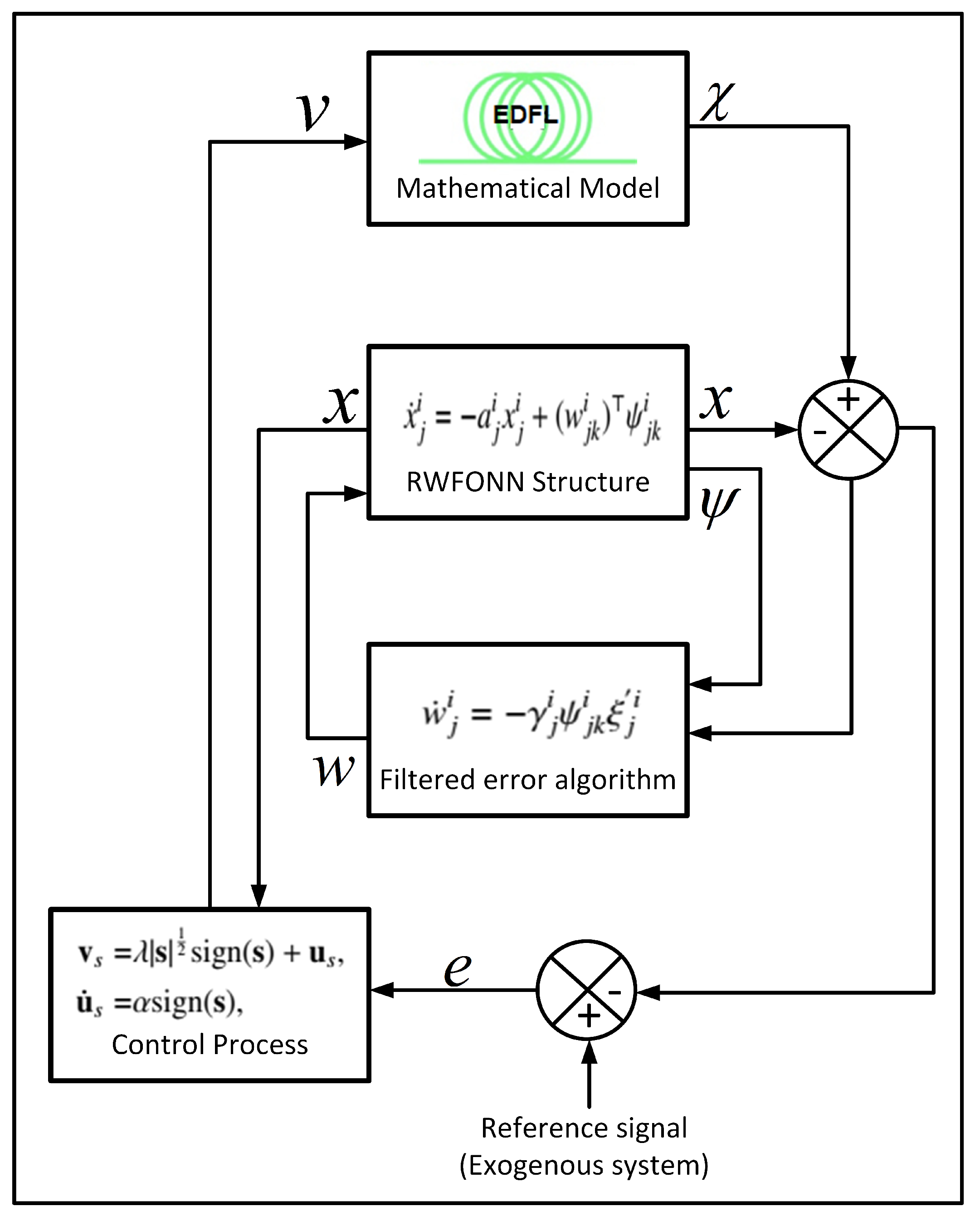
4.1. Recurrent Wavelet First-Order Neural Network

Recurrent wavelet first-order neural networks are used to identify and control electrical systems, robotic manipulators, and unmanned aerial vehicles [34,35]. In the recent work [31], some of us applied the RWFONN to emulate a flywheel energy storage system (FESS), in which the classical sigmoid activation function is replaced by the Morlet wavelet activation function. The general structure of the system is given by
x ˙ j i = a j i x j i + ( w j k i ) ψ j k i ,
where x j i is the state of the i-th neuron, a j i > 0 for i = 1 , 2 , , n is part of the underlying network architecture and it is fixed during the training process, w j k i is the k-th adjustable synaptic weight connecting the j-th state to the i-th neuron, and ψ j k i is a Morlet wavelet activation function defined by ψ ( χ ) = e ( χ 2 / β ) cos ( λ χ ) , where χ is the state of the original system to identify; the parameters β and λ are the expansion and dilation terms. Thus, the laser model (1) is identified online using the RWFONN (15), where the synaptic weights are adjusted via the filtered error algorithm described below.

4.2. Filtered Error Algorithm

The identification scheme starts from the differential equation that describes the unknown system
χ ˙ j i = a j i χ j i + ( w j k i ) * ψ j k i .
Based on (16), the identifier can be chosen as
x ˙ j i = a j i x j i + ( w j k i ) ψ j k i .
In this way, the identification error is defined as ξ j i = x j i χ j i such that
ξ ˙ j i = x ˙ j i χ ˙ j i = a j i x j i + ( w j k i ) ψ j k i ( a j i χ j i + ( w j k i ) * ψ j k i ) = a j i x j i + ( w j k i ) ψ j k i + a j i χ j i ( w j k i ) * ψ j k i = a j i ( x j i χ j i ) + ( w j k i w j k i * ) ψ j k i .
Equation (18) can be rewritten as
ξ ˙ j i = a j i ξ j i + w ˜ j i ψ j k i ,
where w ˜ j i = w j i w j * i . The synaptic weights w j i for i = 1 , 2 , , n are adjusted according to the learning law [36]
w ˙ j i = γ j i ψ j k i ξ j i
called “filtered error”.
Theorem 1.
Consider the RWFONN model whose weights are adjustable according to (20) for each i = 1 , 2 , n , so that
1.
ξ j i , w j i L ( i . e . , ξ j i and w j i are uniformly bounded);
2.
lim t ξ i ( t ) = 0 .
Proof. 
See [36,37]. □
In Appendix A, we present the boundedness of the identification error ξ j i given by the synaptic weights w j i .

4.3. Block Control Linearization Technique

The block control linearization technique aims to convert a nonlinear system into an equivalent one, transforming the mathematical model of the plant to be controlled, expressed by the first-order subsystems consisting of r blocks and representing as [31,38]
x ˙ 1 = f 1 ( x 1 , t ) + B 1 ( x 1 , t ) x 2 + g 1 ( x 1 , t ) , x ˙ i = f i ( x i , t ) + B i ( x i , t ) x i + 1 + g i ( x i , t ) , i = 2 , , r 1 , x ˙ r = f r ( x r , t ) + B r ( x r , t ) u + g r ( x r , t ) ,
where f ( x , t ) is a smooth and bounded mapping, x = x 1 x 2 x r is the state vector decomposed. The matrix B i , since the fictitious x i + 1 for each i-th block has full rank, rank ( B i ) = n i , i = 1 , , r . In this way, the block control linearization technique is applied to the artificial neural network structure (15), to generate the sliding surface that is the argument of the super-twisting control u .

4.4. Super-Twisting Control Algorithm

A first-order sliding modes control has the unwished-for presence of a “chattering effect”, a high-frequency signal generated by the sign function. High-order sliding modes control can decrease the chattering effect, though it requires more equations, and the stability analysis could be more complex. A second-order super-twisting control is an algorithm that improves the sliding modes control because the elimination of chattering and the convergence of the sliding surface to zero are guaranteed by the stability analysis presented before [31,39,40]. Moreover, the external disturbances effects are minimized as can be seen in detail in Appendix B in which the stability analysis guarantees a bounded error in the presence of nonvanishing disturbances.
The sliding surface of the SCTA is generated once the block control linearization technique (21) is applied to the neural network structure proposed for the neuronal identification of the original system states. Thus, the sliding surface is
s = x r ,
where the sliding surface and its dynamics is forced to zero, defined by
s = 0 s ˙ = 0 .
Therefore, the STCA has the following structure
v s = λ | s | 1 2 sign ( s ) + u s , u ˙ s = α sign ( s ) ,
where v s and u s are the controllers of perturbation and chattering, respectively, and λ and α are the diagonal matrices. With STCA, s ( x ) tends to zero as t tends to infinity. In addition, it compensates for the external disturbances and nonlinearities of the system, and with the help of the u s term, the chattering effect is reduced [31,40]. The gain values for the controller are determined by the stability analysis presented in Appendix B.
Figure 1 shows the general flowchart of neural identification and control for different EDFL periodic orbits. The particular notations and processes of identification and control are explained in Section 6.

5. Results of Numerical Simulations

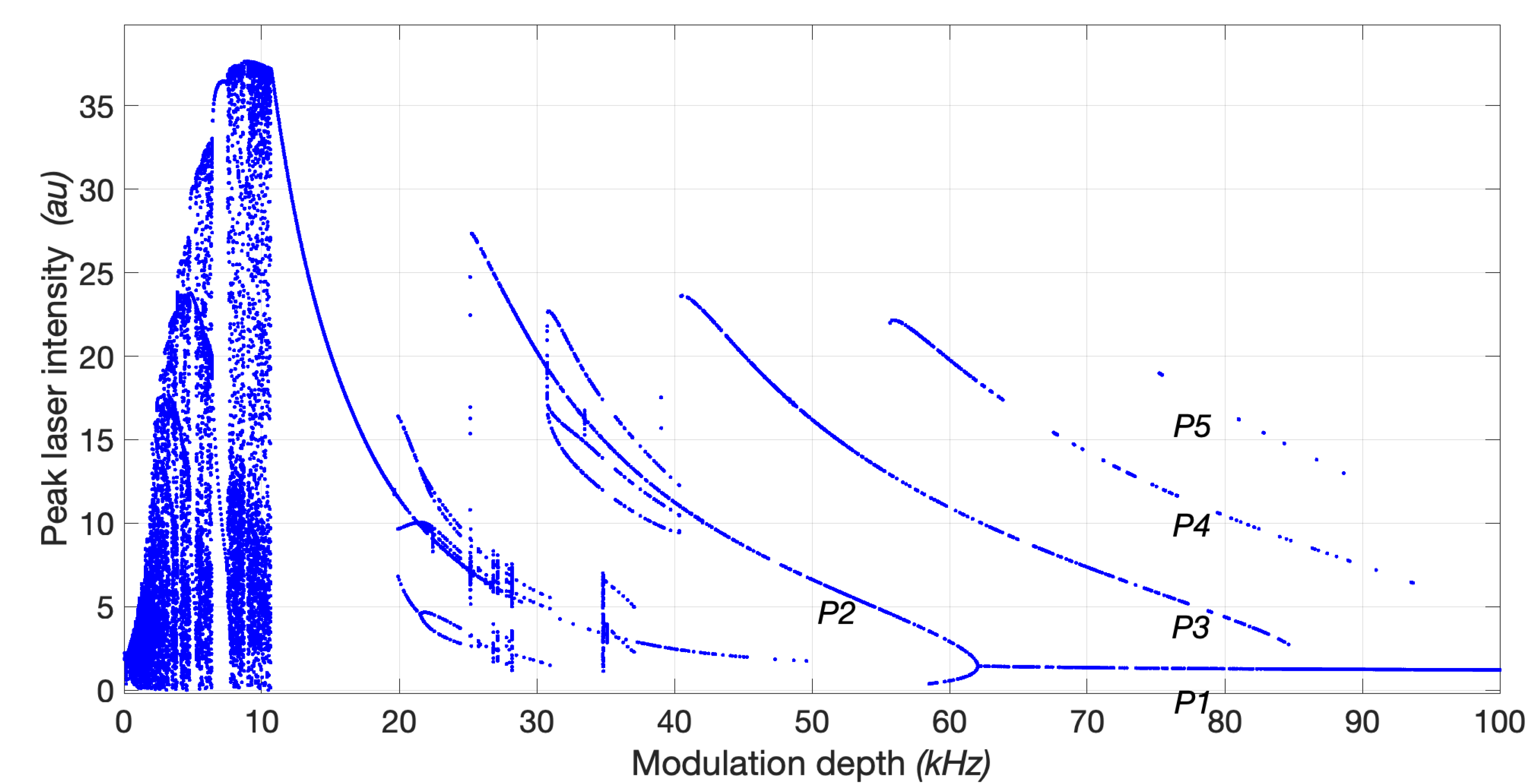
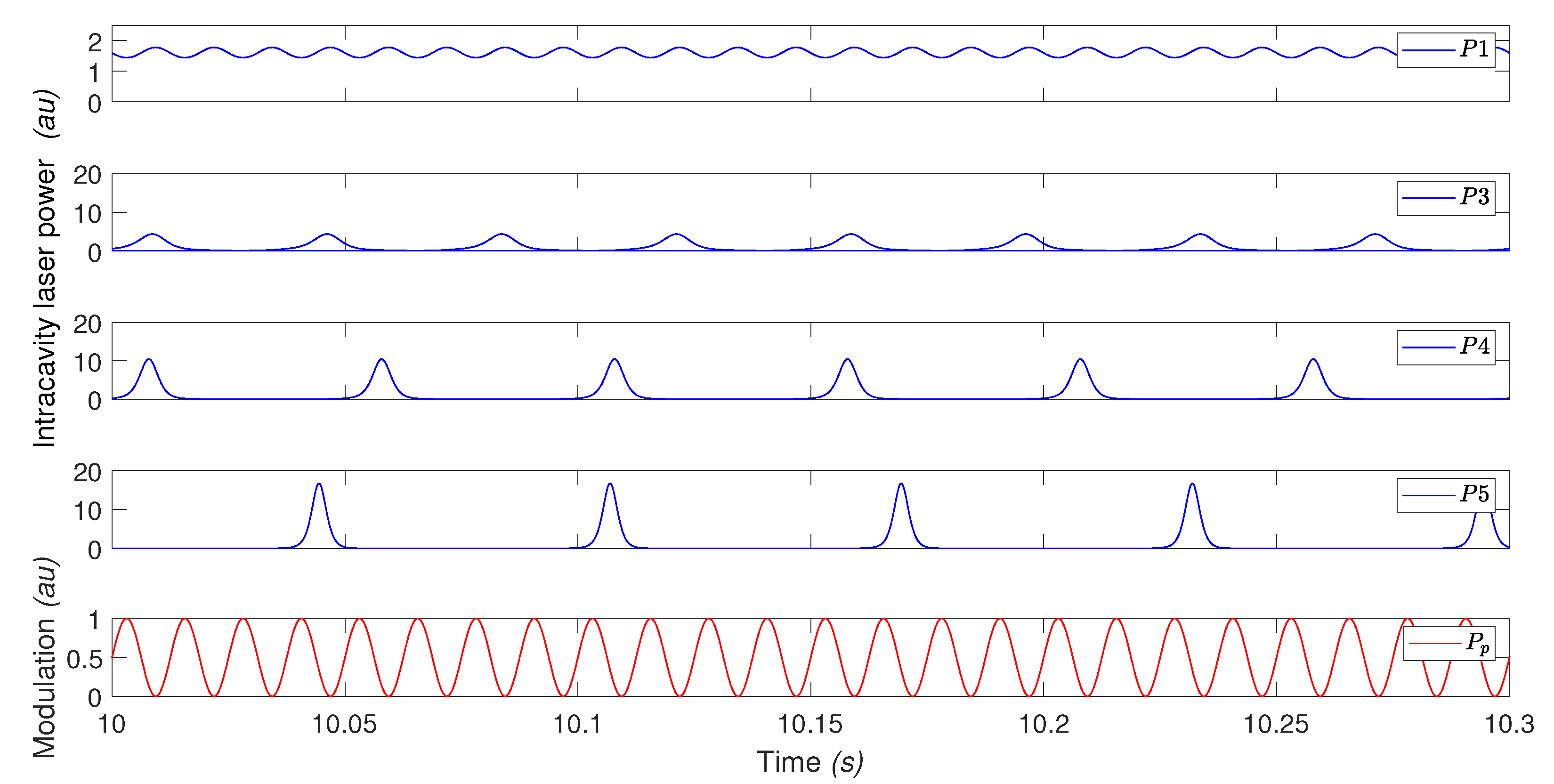
Bifurcation Diagram and Time Series

Numerical calculations of the pump-driven EDFL (1) allow us to obtain time series and bifurcation diagrams. We use the parameters close to the experimental ones taken from [41]. In particular, choosing the pump power P p 0 = 7.4 × 10 19 s 1 , we obtain the laser relaxation oscillation frequency f 0 = 28.724 kHz.
Under harmonic modulation (2) applied to the pump power (1) with driving amplitude m 0 = 1 , we construct the bifurcation diagram of local max of laser power P m a x using f 0 as a control parameter (see Figure 2). This bifurcation diagram is calculated by taking different initial conditions for x and y in (3) and (4). This allows us to find the coexistence of periods and plot the corresponding branches in the diagram. As seen in Figure 2, the branches of period 1, period 3, period 4, and period 5 are shown with the letters P 1 , P 3 , P 4 , and P 5 , respectively, that coexist within a certain frequency range, for example, in the range 74 kHz < f 0 < 83 kHz, for witch P 1 = f 0 , P 3 = 1 3 f 0 , P 4 = 1 4 f 0 , and P 5 = 1 5 f 0 . Each period is born and dies in the corresponding saddle-node bifurcation (Figure 2). The comparison of this diagram with the experimental one displays good agreement, even in detail [11,32].
The time series of the EDFL intensity corresponding to different coexisting periodic regimes observed for modulation frequency f 0 = 80 kHz and amplitude m o = 1 are presented in Figure 3. In the lower panel, we show the pump modulation signal m 0 sin ( 2 π f 0 t ) for reference.

6. Controller Application to RWFONN

In order to identify the EDFL dynamical states, we propose RWFONN with the following structure (15):
x ˙ 1 = a 1 x 1 + b 1 w 1 ψ 1 ( χ 1 ) + x 2 , x ˙ 2 = a 2 x 2 + b 2 w 2 ψ 2 ( χ 2 ) + P p u m p ,
where x 1 and x 2 are states that identify the intracavity laser power P and population inversion N, respectively, a 1 , a 2 , b 1 , b 2 are positive fixed parameters, w 1 and w 2 are the synaptic weights, ψ 1 ( χ 1 ) and ψ 2 ( χ 2 ) are the Morlet wavelet activation functions, and P p u m p is the input, the same as in the original system.
Using the methodology described in Section 4.3, the nonlinear block controllable form is applied to the structure (25), and the tracking error e 1 is given by
e 1 = P r e f x 1 ,
where P r e f represents the reference intracavity EDFL power generated from an exogenous system, which has different periods of the fiber laser as output, and x 1 is the state variable (25). Now the tracking error dynamics e 1 is described as
e ˙ 1 = P ˙ r e f x ˙ 1 .
Substituting the first equation from (25) into (27), we obtain
e ˙ 1 = P ˙ r e f ( a 1 x 1 + b 1 w 1 ψ 1 ( χ 1 ) + x 2 ) = k 1 e 1 ,
where k 1 e 1 is the desired dynamics to vanish the tracking error e 1 . In this way, it is possible to synthesize a control law through the state x 2 , such that
x 2 r e f = P ˙ r e f + a 1 P r e f a 1 e 1 b 1 w 1 ψ 1 ( χ 1 ) + k 1 e 1 .
Additionally, the second error is defined by
e 2 = x 2 r e f x 2 ,
with dynamics
e ˙ 2 = x ˙ 2 r e f x ˙ 2 .
Substituting the second equation from (25) into (31), we obtain
e ˙ 2 = x ˙ 2 r e f ( a 2 x 2 + b 2 w 2 ψ 2 ( χ 2 ) + P p u m p ) .
Based on the error dynamics e 1 and e 2 , the following system of equations represents the block control transformation with structure (21):
e ˙ 1 = k 1 e 1 + e 2 , e ˙ 2 = P ¨ r e f + ( a 1 + a 2 ) P ˙ r e f + ( a 1 a 2 ) P r e f + ( k 1 2 + a 1 k 1 a 1 a 2 + a 2 k 1 ) e 1 a 2 e 2 b 1 w 1 ψ 1 ( χ 1 ) a 1 b 1 w 1 ψ 1 ( χ 1 ) b 2 w 2 ψ 2 ( χ 2 ) ( λ 1 | s | 1 2 sign ( s ) + u s ) .
According to Equation (33), regarding the tracking error variables e 1 and e 2 , the control input P p u m p = λ | s | 1 2 sign ( s ) + u s guarantees that these errors will be steered to zero in finite time.
Selecting the sliding surface s = e 2 from (33) where the control signal appears, the new system can be rewritten as
s ˙ = P ¨ r e f + ( a 1 + a 2 ) P ˙ r e f + ( a 1 a 2 ) P r e f + ( k 1 2 + a 1 k 1 a 1 a 2 + a 2 k 1 ) e 1 a 2 e 2 b 1 w 1 ψ 1 ( χ 1 ) a 1 b 1 w 1 ψ 1 ( χ 1 ) b 2 w 2 ψ 2 ( χ 2 ) ( λ | s | 1 2 sign ( s ) + u s ) , u ˙ s = α sign ( s ) .
Although stability analysis for STCA is presented in [42], in Appendix B we complement it including the boundedness of the neural identification error.

7. Neural Identification and Controller

In this section, we present the results of numerical simulation of the neural identification of the system (1) through the neural network structure (25). In addition, we describe the neural controller which displays noise-induced multistate intermittency in the EDFL [23]. The control forces the multistable system toward a desired state, using an exogenous system. The simulations are performed using Matlab/Simulink (MatlabTM) with a Runge–Kutta algorithm with a 10 7 s step size.

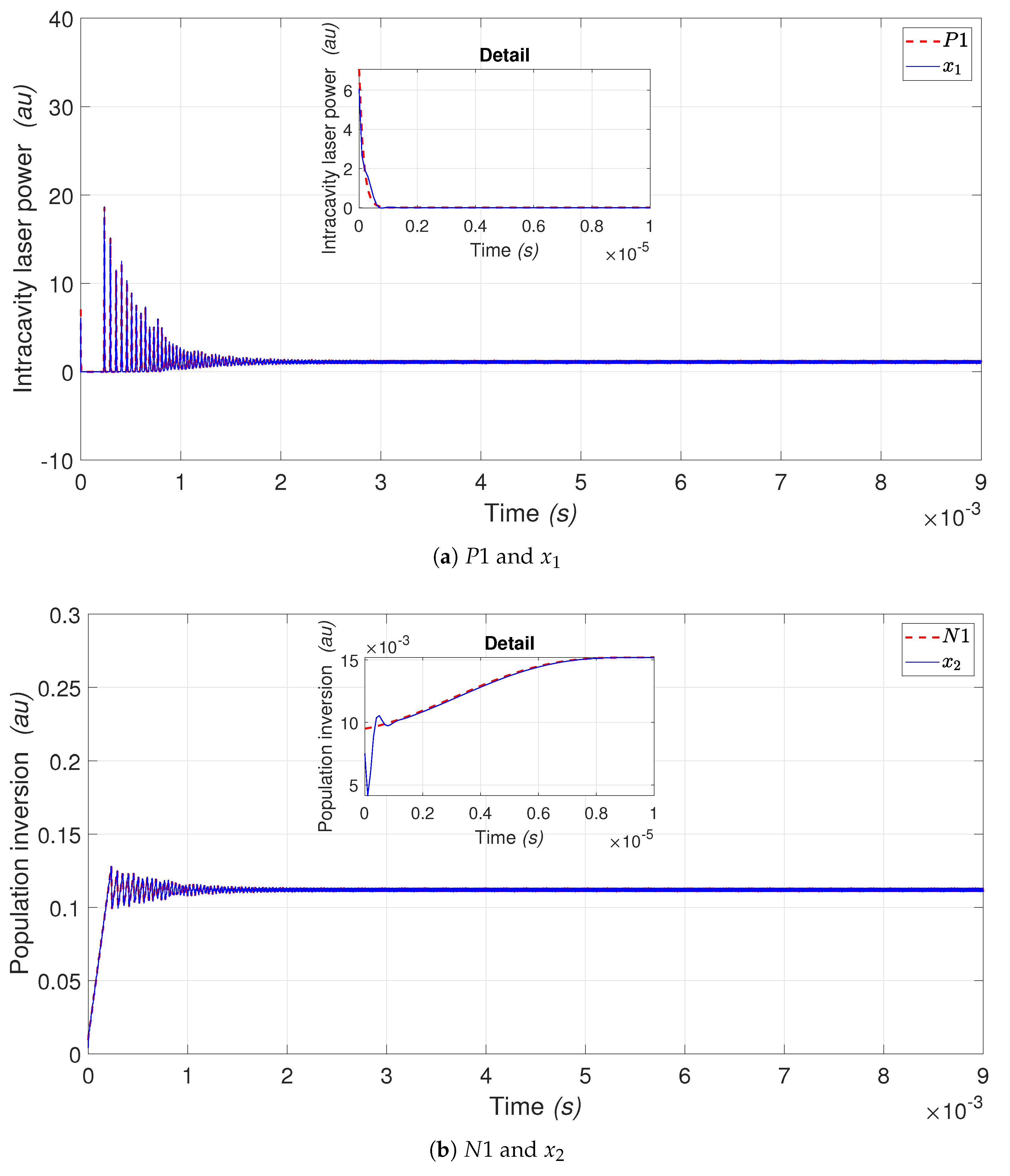
7.1. Neural Identification of P1

For neural identification of the EDFL states, we take the parameter values a 1 = a 2 = b 1 = b 2 = 1.005 × 10 7 , the filtered error parameters γ 1 = γ 2 = 1.005 × 10 7 and the parameters of Morlet wavelet activation functions λ 1 = λ 2 = 10 5 and β 1 = β 2 = 8.9 × 10 5 . Figure 4a,b show the neural identification of the EDFL states. Figure 4a shows the neural identification of the intracavity laser power of the period ( P 1 ) indicated by the red dashed line, while the blue continuous line represents the state of the neural network ( x 1 ). Using the initial condition x ( 0 ) = 7.0614 for period P 1 , the neural network state is x 1 = 6.0614 . The neural identification for P 1 is obtained with the convergence time of 0.00002 s.
The red dashed line in Figure 4b shows the neural identification of population inversion, and the blue continuous line represents the neural network sate ( x 2 ). Using the initial condition for N 1 y ( 0 ) = 0.0095 , the neural network state is x 2 = 0.0075 ; the neural identification is obtained with the convergence time of 10 5 s.
The neuronal identification of for periods P 3 , P 4 , and P 5 is obtained using the same neural network parameters.
Table 2 shows the neural identification results for P 3 (see Figure 5a,b), P 4 (see Figure 6a,b) and P 5 (see Figure 7a,b) periodic orbits, where we present the initial conditions for each EDFL period and the convergence time to the corresponding attractor.

7.2. Neural Identification of Multistate Intermittency

In order to identify multistate intermittency, we add external noise to Equation (2) that results in
P p = P p 0 [ 1 + m 0 sin ( 2 π F 0 t ) + η ζ ,
where η = 0.8 is the noise amplitude and ζ is the random number. Noise induces multistate intermittency so that the four periodic behaviors ( P 1 , P 3 , P 4 , and P 5 ) alternate. The values of the neural network parameters are the same as in the previous subsection. It is worth mentioning that the laser response does not depend on the initial conditions of the system; it only depends on the external noise amplitude [23].
The intracavity laser power ( P h ) under the influence of noise is shown in Figure 8a by the red dashed line, and the blue continuous line represents the neural network state ( x 1 ). Neural identification is obtained with a convergence time of 0.00001 s, as seen in the inset.
Figure 8b shows the population inversion under white noise ( N h ) by the red dashed line, while the blue continuous line represents the neural network state ( x 2 ). The inset shows the neural identification obtained with a convergence time of 0.00002 s. The results of simulations of the neural identification of the plant, represented by the system (1), offer a good approximation. This confirms that the proposed neural network structure (25) is viable for attractor identification in the EDFL. Ensuring neural identification is guaranteed when external noise is applied to the EDFL (1).

7.3. EDFL Controller

Here, we present the results of the controller application to the noisy EDFL, based on the proposed neural network structure (25). The controller allows the selection of one of the coexisting regimes which appears in multistate intermittency. In particular, to select the period-3 ( P 3 ) orbit through the artificial neural network, we use the following gain parameters: k 1 = 6666666666 , λ 1 = 0.01 , and α 1 = 0.6 . Figure 9 illustrates the EDFL behavior toward P 3 . P r e f is shown by the red dashed line, and P of EDFL is represented by the blue continuous line. This figure shows the tracking trajectory of the EDFL (P) to the reference ( P r e f ), where the reference is P 3 generated by the exogenous system. The inset shows a rapid convergence.
Figure 10 illustrates the EDFL behavior toward the period-4 P 4 orbit. P r e f is represented by the red dashed line, and P of EDFL by the blue continuous line. This figure shows the tracking trajectory of the EDFL (P) to the reference ( P r e f ), where the reference is P 4 generated by the exogenous system. The inset illustrates a rapid convergence. The chosen gain parameters are k 1 = 2.1 × 10 12 , λ 1 = 0.001 , and α 1 = 0.6 .
Figure 11 shows the EDFL behavior toward the period-5 ( P 5 ) orbit. P r e f is represented by the red dashed line, and P by the blue continuous line. This figure shows the tracking trajectory of the EDFL (P) to the reference ( P r e f ), where the reference is P 5 generated by the exogenous system. The inset illustrates a rapid convergence. The chosen gain parameters are k 1 = 3.9 × 10 12 , λ 1 = 0.001 , and α 1 = 0.6 .
It should be noted that by the proper choice of controller gains, the laser can be made monostable in any of the coexisting attractors ( P 3 , P 4 , or P 5 ).

8. Conclusions

A novel neural controller is proposed to control multistability in an erbium-doped fiber laser (EDFL) with coexisting attractors and make the laser monostable. This can be achieved using RWFONN, the application of the block control linearization technique and STCA, allowing attractor selection. We showed that the EDFL states can be identified through the proposed artificial neural network. Once the states are classified, the block control linearization technique is applied to generate the sliding surface, which is an argument to implement a robust super-twisting control. On the other hand, the proposed control is indirectly applied to the EDFL since the controller is based on the artificial neural network. We believe that the proposed neural control technique can also be used in other dynamical systems with coexisting attractors.

Author Contributions

D.A.M. and D.L.-M. contributed with the design process of the neural controller, methodology, validation and editing; R.J.-R., J.H.G.-L. and G.H.-C. contributed with conceptualization, review, validation of simulation results, review and editing; A.N.P. contributed with conceptualization, review. All authors have read and agreed to the published version of the manuscript.

Funding

Programa Presupuestario F003 CONACYT–MEXICO Convocatoria “Ciencia Básica y/o Ciencia de Frontera. Modalidad: Paradigmas y Controversias de la Ciencia 2022”, Referencia: 320597 Responsable Técnico: Rider Jaimes Reategui, Institución: Universidad de Guadalajara, Título: Memoria y Compuerta Lógica Óptica en un Laser de Fibra Dopada con Erbio Operando en Régimen no Lineal y Multi Estable.

Institutional Review Board Statement

Not applicable.

Informed Consent Statement

Not applicable.

Data Availability Statement

Not applicable.

Acknowledgments

The authors acknowledge support from CONACYT PCC-2022/320597 and from Universidad de Guadalajara, Centro Universitario de los Lagos.

Conflicts of Interest

The authors declare no conflict of interest.

Appendix A. Identification Error Boundedness

Theorem A1.
Suppose that the system (1) and model (15) are initially in the same state x ( 0 ) = χ ( 0 ) . Then, for any ϵ > 0 and any finite T > 0 , there exist an integer L and a matrix w R L × n such that the state x ( t ) of the RWFONN model (15) and weight values w = w satisfy
sup 0 t T x ( t ) χ ( t ) ϵ .
Next, using the Bellman–Gronwall lemma [43], the identification error ξ j i = x j i χ j i is bounded by
ξ ϵ 2 .
Proof. 
See reference [44]. □

Appendix B. Closed-Loop Stability Analysis

Proof. 
The convergence of ξ j i is considered to complement the analytic test [42]. Thus, an identification error occurs (A1), and the Lyapunov function can be written as
V ( ζ , ξ ) = ζ P ζ + 1 2 ( ξ 1 i ) 2 .
The first time derivative of Equation (A2) is
V ˙ ( ζ , ξ ) = 1 | ζ | ζ Q ζ + ξ 1 i ξ ˙ 1 i .
Substituting the time derivative of ξ j i = x j i χ j i obtained through the filtered error algorithm (20) applied to Equation (A3), we obtain
V ˙ ( ζ , ξ ) = 1 | ζ | ζ Q ζ + ξ 1 i ( a 1 i x 1 i + b 1 i w 1 i ψ 1 i ( χ 1 i ) + x 2 i ) χ ˙ 1 i .
In order to guarantee that (A4) is negative definite, the desired dynamics for x 2 d is
x 2 d i = c 1 ξ 1 i + a 1 i x 1 i b 1 i w 1 i ψ 1 i + χ ˙ 1 i .
Thus,
V ˙ ( ζ , ξ ) = 1 | ζ | ζ Q ζ + ξ 1 i ( a 1 i x 1 i + b 1 i w 1 i ψ 1 i + ( c 1 ξ 1 i + a 1 i x 1 i b 1 i w 1 i ψ 1 i + χ ˙ 1 i ) χ ˙ 1 i ) = 1 | ζ | ζ Q ζ c 1 ξ 1 2 ,
with c 1 > 0 real, the stability uniformly ultimately bounded is ensured. □

References

  1. Digonnet, M.J. Rare-Earth-Doped Fiber Lasers and Amplifiers, Revised and Expanded; CRC Press: Boca Raton, FL, USA, 2001. [Google Scholar]
  2. Luo, L.G.; Chu, P.L. Optical secure communications with chaotic erbium-doped fiber lasers. J. Opt. Soc. Am. B 1998, 15, 2524–2530. [Google Scholar] [CrossRef]
  3. Shay, T.M.; Duarte, F.J. Tunable fiber lasers. In Tunable Laser Applications; Duarte, F.J., Ed.; CRC Press: Boca Raton, FL, USA, 2009. [Google Scholar]
  4. Pisarchik, A.N.; Jaimes-Reátegui, R.; Sevilla-Escoboza, R.; García-Lopez, J.H.; Kazantsev, V.B. Optical fiber synaptic sensor. Opt. Lasers Eng. 2011, 49, 736–742. [Google Scholar] [CrossRef]
  5. Mary, R.; Choudhury, D.; Kar, A.K. Applications of fiber lasers for the development of compact photonic devices. IEEE J. Select. Top. Quantum Electron. 2014, 20, 72–84. [Google Scholar] [CrossRef]
  6. Zhao, L.; Li, D.; Li, L.; Wang, X.; Geng, Y.; Shen, D.; Su, L. Route to larger pulse energy in ultrafast fiber lasers. IEEE J. Select. Top. Quantum Electron. 2017, 24, 1–9. [Google Scholar] [CrossRef]
  7. Zervas, M.N.; Codemard, C.A. High power fiber lasers: A review. IEEE J. Select. Top. Quantum Electron. 2014, 20, 219–241. [Google Scholar] [CrossRef]
  8. Castillo-Guzmán, A.; Anzueto-Sánchez, G.; Selvas-Aguilar, R.; Estudillo-Ayala, J.; Rojas-Laguna, R.; May-Arrioja, D.; Martínez-Ríos, A. Erbium-Doped Tunable Fiber Laser. In Proceedings of the Laser Beam Shaping IX. International Society for Optics and Photonics, San Diego, CA, USA, 11–12 August 2008; Volume 7062, p. 70620Y. [Google Scholar]
  9. Saucedo-Solorio, J.M.; Pisarchik, A.N.; Kir’yanov, A.V.; Aboites, V. Generalized multistability in a fiber laser with modulated losses. J. Opt. Soc. Am. B 2003, 20, 490–496. [Google Scholar] [CrossRef]
  10. Reategui, R.J.; Kir’yanov, A.V.; Pisarchik, A.N.; Barmenkov, Y.O.; Il’ichev, N.N. Experimental study and modeling of coexisting attractors and bifurcations in an erbium-doped fiber laser with diode-pump modulation. Laser Phys. 2004, 14, 1277–1281. [Google Scholar]
  11. Pisarchik, A.; Jaimes-Reátegui, R.; Sevilla-Escoboza, R.; Huerta-Cuellar, G. Multistate intermittency and extreme pulses in a fiber laser. Phys. Rev. E 2012, 86, 056219. [Google Scholar] [CrossRef]
  12. Ke, J.; Yi, L.; Xia, G.; Hu, W. Chaotic optical communications over 100-km fiber transmission at 30-Gb/s bit rate. Opt. Lett. 2018, 43, 1323–1326. [Google Scholar] [CrossRef]
  13. Keren, S.; Horowitz, M. Interrogation of fiber gratings by use of low-coherence spectral interferometry of noiselike pulses. Opt. Lett. 2001, 26, 328–330. [Google Scholar] [CrossRef] [PubMed]
  14. Lim, H.; Jiang, Y.; Wang, Y.; Huang, Y.C.; Chen, Z.; Wise, F.W. Ultrahigh-resolution optical coherence tomography with a fiber laser source at 1 μm. Opt. Lett. 2005, 30, 1171–1173. [Google Scholar] [CrossRef] [PubMed]
  15. Wu, Q.; Okabe, Y.; Sun, J. Investigation of dynamic properties of erbium fiber laser for ultrasonic sensing. Opt. Express 2014, 22, 8405–8419. [Google Scholar] [CrossRef] [PubMed]
  16. Droste, S.; Ycas, G.; Washburn, B.R.; Coddington, I.; Newbury, N.R. Optical frequency comb generation based on erbium fiber lasers. Nanophotonics 2016, 5, 196–213. [Google Scholar] [CrossRef]
  17. Kraus, M.; Ahmed, M.A.; Michalowski, A.; Voss, A.; Weber, R.; Graf, T. Microdrilling in steel using ultrashort pulsed laser beams with radial and azimuthal polarization. Opt. Express 2010, 18, 22305–22313. [Google Scholar] [CrossRef] [PubMed]
  18. Philippov, V.; Codemard, C.; Jeong, Y.; Alegria, C.; Sahu, J.K.; Nilsson, J.; Pearson, G.N. High-energy in-fiber pulse amplification for coherent lidar applications. Opt. Lett. 2004, 29, 2590–2592. [Google Scholar] [CrossRef] [PubMed]
  19. Morin, F.; Druon, F.; Hanna, M.; Georges, P. Microjoule femtosecond fiber laser at 1.6 μm for corneal surgery applications. Opt. Lett. 2009, 34, 1991–1993. [Google Scholar] [CrossRef] [PubMed]
  20. Sanchez, F.; Le Boudec, P.; François, P.L.; Stephan, G. Effects of ion pairs on the dynamics of erbium-doped fiber lasers. Phys. Rev. A 1993, 48, 2220. [Google Scholar] [CrossRef] [PubMed]
  21. Colin, S.; Contesse, E.; Le Boudec, P.; Stephan, G.; Sanchez, F. Evidence of a saturable-absorption effect in heavily erbium-doped fibers. Opt. Lett. 1996, 21, 1987–1989. [Google Scholar] [CrossRef] [PubMed]
  22. Rangel-Rojo, R.; Mohebi, M. Study of the onset of self-pulsing behaviour in an Er-doped fibre laser. Opt. Commun. 1997, 137, 98–102. [Google Scholar] [CrossRef]
  23. Huerta-Cuellar, G.; Pisarchik, A.N.; Barmenkov, Y.O. Experimental characterization of hopping dynamics in a multistable fiber laser. Phys. Rev. E 2008, 78, 035202. [Google Scholar] [CrossRef]
  24. Pisarchik, A.N.; Hramov, A.E. Multistability in Physical and Living Systems: Characterization and Applications; Springer: Berlin/Heidelberg, Germany, 2022. [Google Scholar]
  25. Chen, B.; Cheng, X.; Bao, H.; Chen, M.; Xu, Q. Extreme Multistability and Its Incremental Integral Reconstruction in a Non-Autonomous Memcapacitive Oscillator. Mathematics 2022, 10, 754. [Google Scholar] [CrossRef]
  26. Pisarchik, A.N.; Feudel, U. Control of multistability. Phys. Rep. 2014, 540, 167–218. [Google Scholar] [CrossRef]
  27. Pisarchik, A.N.; Jaimes-Reátegui, R.; Rodríguez-Flores, C.; García-López, J.H.; Huerta-Cuellar, G.; Martín-Pasquín, F.J. Secure chaotic communication based on extreme multistability. J. Franklin Inst. 2021, 358, 2561–2575. [Google Scholar] [CrossRef]
  28. Bao, H.; Ding, R.; Hua, M.; Wu, H.; Chen, B. Initial-condition effects on a two-memristor-based Jerk system. Mathematics 2022, 10, 411. [Google Scholar] [CrossRef]
  29. Bao, H.; Hua, Z.; Li, H.; Chen, M.; Bao, B. Memristor-based hyperchaotic maps and application in auxiliary classifier generative adversarial nets. IEEE Trans. Ind. Inform. 2021, 18, 5297–5306. [Google Scholar] [CrossRef]
  30. Jaimes-Reátegui, R.; Esqueda de la Torre, J.O.; García-López, J.H.; Huerta-Cuellar, G.; Aboites, V.; Pisarchik, A.N. Generation of giant periodic pulses in the array of erbium-doped fiber lasers by controlling multistability. Opt. Commun. 2020, 477, 126355. [Google Scholar] [CrossRef]
  31. Magallón, D.A.; Castañeda, C.E.; Jurado, F.; Morfin, O.A. Design of a neural super-twisting controller to emulate a flywheel energy storage system. Energies 2021, 14, 6416. [Google Scholar] [CrossRef]
  32. Pisarchik, A.N.; Jaimes-Reátegui, R.; Sevilla-Escoboza, R.; Huerta-Cuellar, G.; Taki, M. Rogue waves in a multistable system. Phys. Rev. Lett. 2011, 107, 274101. [Google Scholar] [CrossRef] [PubMed]
  33. Pisarchik, A.N.; Kir’yanov, A.V.; Barmenkov, Y.O.; Jaimes-Reátegui, R. Dynamics of an erbium-doped fiber laser with pump modulation: Theory and experiment. J. Opt. Soc. Am. B 2005, 22, 2107–2114. [Google Scholar] [CrossRef]
  34. Jurado, F.; Lopez, S. A wavelet neural control scheme for a quadrotor unmanned aerial vehicle. Philos. Trans. R. Soc. A 2018, 376, 20170248. [Google Scholar] [CrossRef]
  35. Vázquez, L.A.; Jurado, F. Continuous-time decentralized wavelet neural control for a 2 DOF robot manipulator. In Proceedings of the 2014 11th International Conference on Electrical Engineering, Computing Science and Automatic Control (CCE), Ciudad del Carmen, Mexico, 29 September–3 October 2014; pp. 1–6. [Google Scholar]
  36. Kosmatopoulos, E.B.; Polycarpou, M.M.; Christodoulou, M.A.; Ioannou, P.A. High-order neural network structures for identification of dynamical systems. IEEE Trans. Neural Netw. 1995, 6, 422–431. [Google Scholar] [CrossRef] [PubMed]
  37. Vázquez, L.A.; Jurado, F.; Alanís, A.Y. Decentralized identification and control in real-time of a robot manipulator via recurrent wavelet first-order neural network. Math. Probl. Eng. 2015, 2015, 451049. [Google Scholar] [CrossRef]
  38. Loukianov, A.G. Robust block decomposition sliding mode control design. Math. Probl. Eng. 2003, 8, 349–365. [Google Scholar] [CrossRef]
  39. Utkin, V.; Guldner, J.; Shi, J. Sliding Mode Control in Electro-Mechanical Systems; CRC Press: Boca Raton, FL, USA, 2017. [Google Scholar]
  40. Chalanga, A.; Kamal, S.; Fridman, L.M.; Bandyopadhyay, B.; Moreno, J.A. Implementation of super-twisting control: Super-twisting and higher order sliding-mode observer-based approaches. IEEE Trans. Ind. Electron. 2016, 63, 3677–3685. [Google Scholar] [CrossRef]
  41. Pisarchik, A.N.; Barmenkov, Y.O.; Kir’yanov, A.V. Experimental characterization of the bifurcation structure in an erbium-doped fiber laser with pump modulation. IEEE J. Quantum Electron. 2003, 39, 1567–1571. [Google Scholar] [CrossRef]
  42. Moreno, J.A.; Osorio, M. Strict Lyapunov functions for the super-twisting algorithm. IEEE Trans. Autom. Control 2012, 57, 1035–1040. [Google Scholar] [CrossRef]
  43. Hale, J.K. Ordinary Differential Equations; Wiley-InterScience: Maitland, FL, USA, 1969. [Google Scholar]
  44. Rovithakis, G.A.; Christodoulou, M.A. Adaptive Control with Recurrent High-Order Neural Networks: Theory and Industrial Applications; Springer Science & Business Media: Berlin/Heidelberg, Germany, 2012. [Google Scholar]
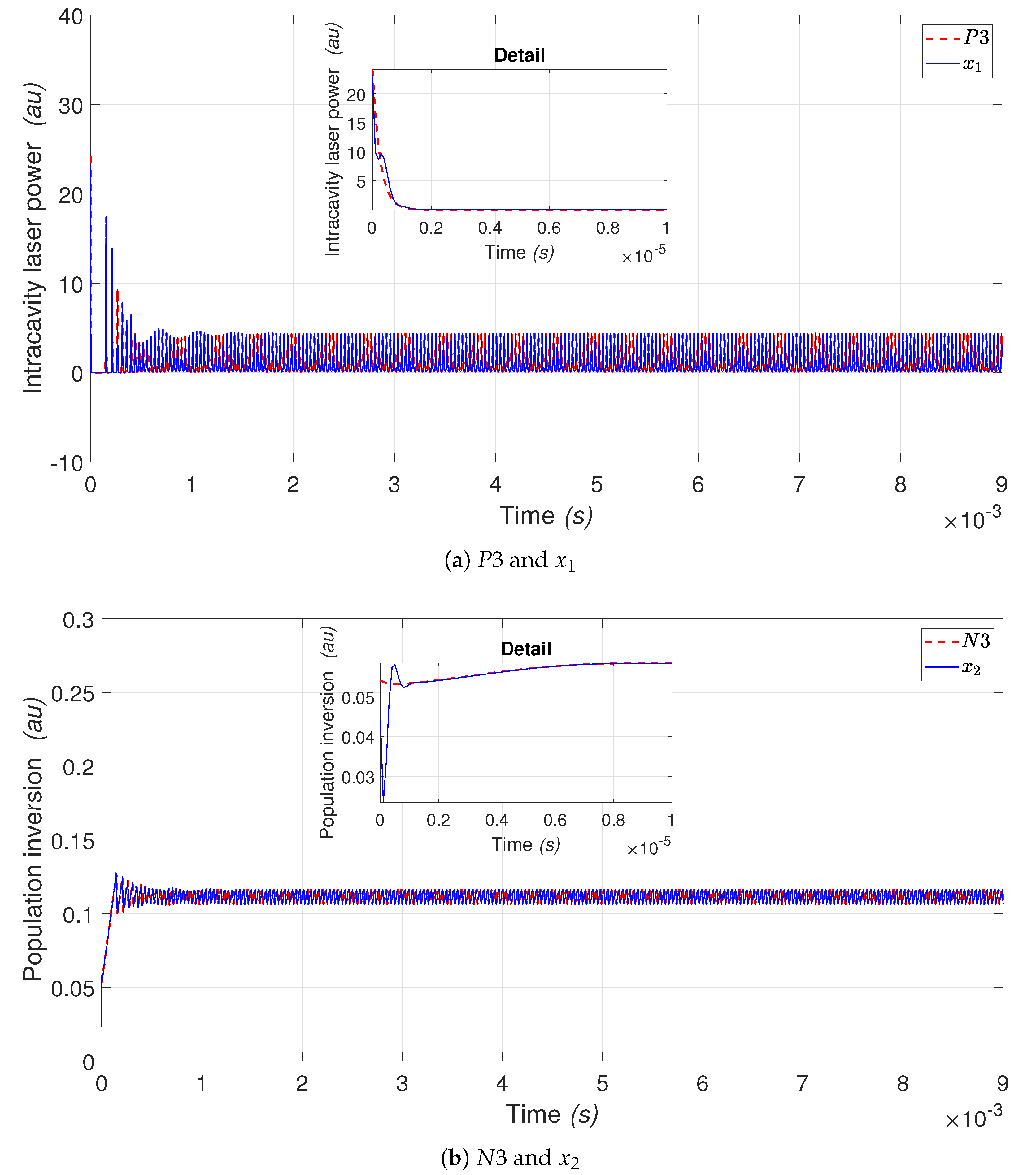
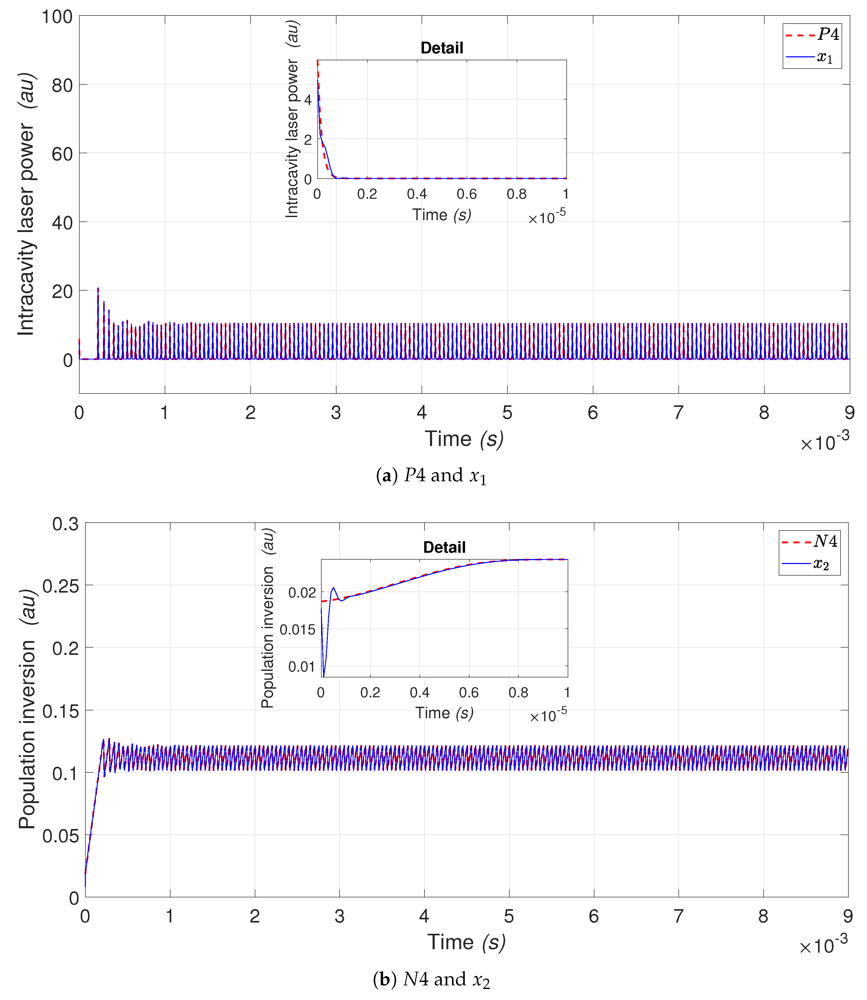
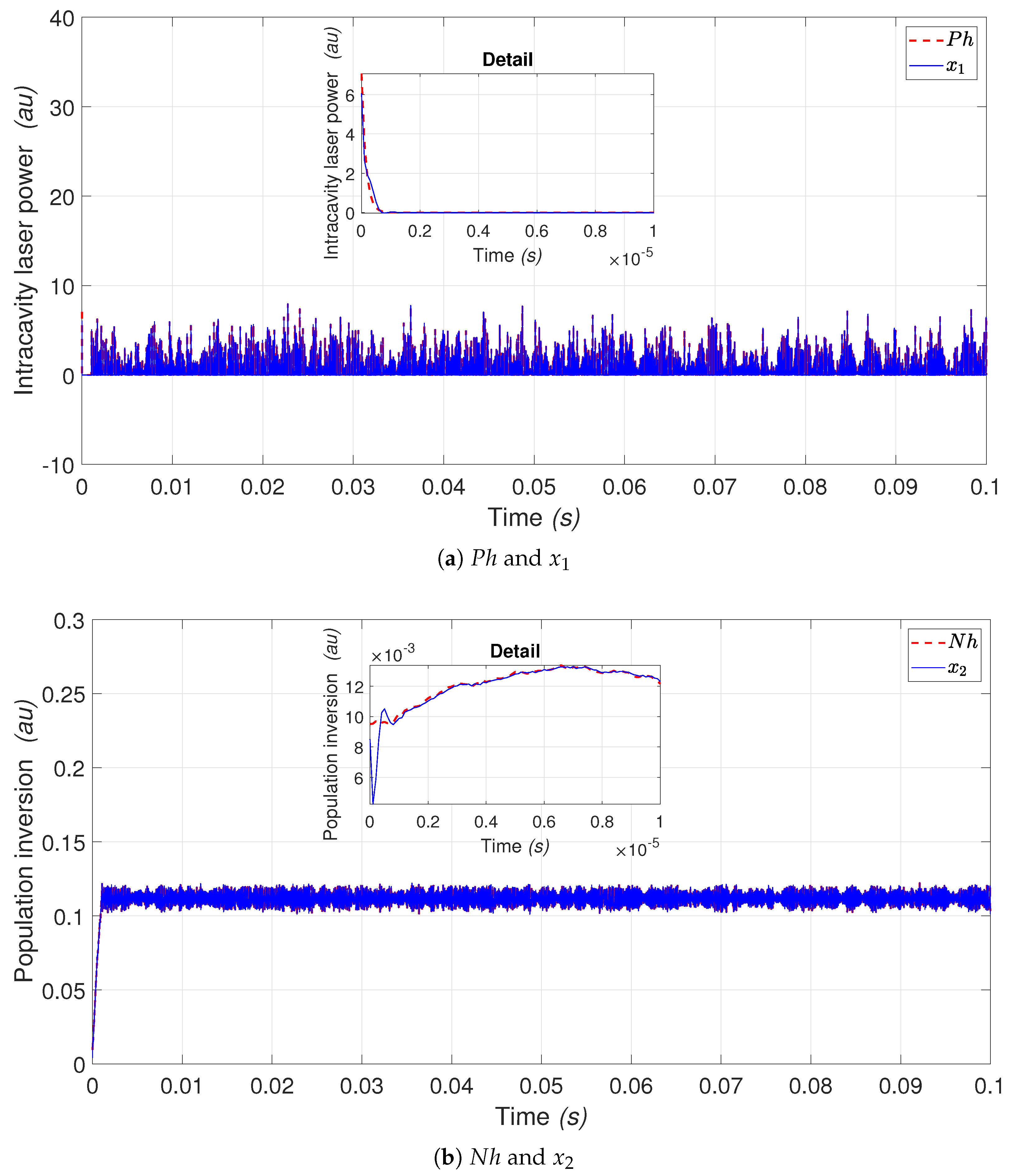
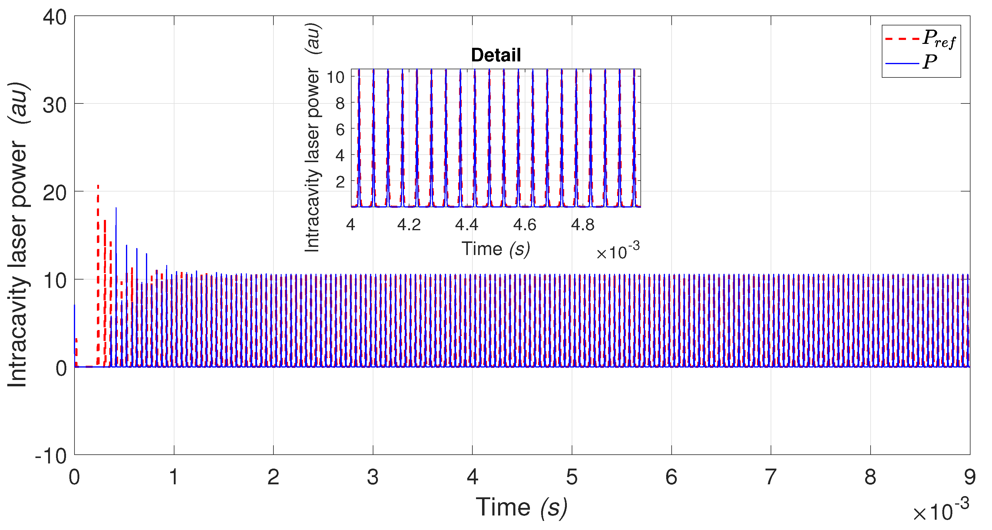
Figure 1. Methodology flowchart of neural identification and control.
Mathematics 10 03140 g001
Figure 2. Bifurcation diagrams of peak laser intensity P with driving frequency f 0 as a control parameter for m 0 = 1 . P1, P3, P4, and P5 are branches of the corresponding coexisting attractors found by taking different initial conditions.
Mathematics 10 03140 g002
Figure 3. Time series of the laser intensity corresponding to coexisting P 1 , P 3 , P 4 , and P 5 regimes at f 0 = 80 kHz and m 0 = 1 .
Mathematics 10 03140 g003
Figure 4. (a) Intracavity laser power P 1 and neural identification x 1 behavior. (b) Population inversion N 1 and neural identification x 2 .
Mathematics 10 03140 g004
Figure 5. (a) Intracavity laser power P 3 and neural identification x 1 behavior. (b) Population inversion N 3 and neural identification x 2 .
Mathematics 10 03140 g005
Figure 6. (a) Intracavity laser power P 4 and neural identification x 1 behavior. (b) Population inversion N 4 and neural identification x 2 .
Mathematics 10 03140 g006
Figure 7. (a) Intracavity laser power P 5 and neural identification x 1 behavior. (b) Population inversion N 5 and neural identification x 2 .
Mathematics 10 03140 g007
Figure 8. (a) Intracavity laser power P h and neural identification x 1 behavior. (b) Population inversion N h and neural identification x 2 .
Mathematics 10 03140 g008
Figure 9. EDFL tracking to P3.
Mathematics 10 03140 g009
Figure 10. EDFL tracking to P4.
Mathematics 10 03140 g010
Figure 11. EDFL tracking to P5.
Mathematics 10 03140 g011
Table 1. Parameters used in numerical simulations.
c 1 c 2 c 3 d 1 d 2 d 3 P 0
2.4 6.9 × 10 13 5.1 × 10 13 3.5 × 10 7 2.6 × 10 7 0.5 2 × 10 23 P p
Table 2. Neural identification results for P 1 , P 3 , P 4 and P 5 periods.
FigurePeriod (States)LineInitial ConditionConvergence
Figure 4a P 1 and x 1 Red dashed and blue continuous x = 7.0614 and x 1 = 6.0614 0.00002 s
Figure 4b N 1 and x 2 Red dashed and blue continuous y = 0.0095 and x 2 = 0.0075 0.00001 s
Figure 5a P 3 and x 1 Red dashed and blue continuous x = 24.2265 and x 1 = 23.2265 0.00002 s
Figure 5b N 3 and x 2 Red dashed and blue continuous y = 0.0542 and x 2 = 0.0442 0.00001 s
Figure 6a P 4 and x 1 Red dashed and blue continuous x = 5.987 and x 1 = 4.987 0.00001 s
Figure 6b N 4 and x 2 Red dashed and blue continuous y = 0.0187 and x 2 = 0.0177 0.00001 s
Figure 7a P 5 and x 1 Red dashed and blue continuous x = 91.1913 and x 1 = 90.1913 0.00001 s
Figure 7b N 5 and x 2 Red dashed and blue continuous y = 0.096 and x 2 = 0.086 0.00002 s
Publisher’s Note: MDPI stays neutral with regard to jurisdictional claims in published maps and institutional affiliations.

