Article

The Geo/Ga,Y/1/N Queue Revisited

1
Department of Mathematics and Computer Science, Royal Military College of Canada, P.O. Box 17000, Kingston, ON K7K 7B4, Canada
2
School of Computer Applications, Kalinga Institute of Industrial Technology, Bhubaneswar 751 024, India
*
Author to whom correspondence should be addressed.
Mathematics 2022, 10(17), 3142; https://doi.org/10.3390/math10173142
Submission received: 25 July 2022 / Revised: 20 August 2022 / Accepted: 23 August 2022 / Published: 1 September 2022

Abstract

:
We not only present an alternative and simpler approach to find steady-state distributions of the number of jobs for the finite-space queueing model G e o / G a , Y / 1 / N using roots of the inherent characteristic equation, but also correct errors in some published papers. The server has a random service capacity Y, and it processes the jobs only when the number of jobs in the system is at least ‘a’, a threshold value. The main advantage of this alternative process is that it gives a unified approach in dealing with both finite- and infinite-buffer systems. The queue-length distribution is obtained both at departure and random epochs. We derive the relation between the discrete-time Geo/ G a , Y /1/N queue and its continuous-time analogue. Finally, we deal with performance measures and numerical results.

1. Introduction

Discrete-time queues with batch service have numerous applications in various areas such as transportation systems, traffic, production, manufacturing, telecommunication, and cloud computing. In various real-life settings, it is often noted that the jobs are served in batches. The server may serve with fixed maximum or variable capacity in batch service systems. For more details on batch service queues, one may refer to Chaudhry and Templeton [1] as well as Medhi [2]. Discrete-time queues are more notable in systems’ modelling, see [3,4,5].
In discrete-time queues, it is assumed that arrivals and departures occur at boundary epochs of time slots. Further, discrete-time queues deal with an early arrival system (EAS) or a late arrival system with delayed access (LAS-DA). For more on this, see Hunter [4]. We may note that EAS and LAS-DA policies are similar to departure-first (DF) and arrival-first (AF), respectively; see Gravey and Hébuterne [6].
Several researchers study single-server batch-service discrete-time queues with various phenomena, see [7,8,9,10,11,12,13]. In Gupta and Goswami [10], they discuss a discrete-time finite-buffer general bulk service queue under both LAS-DA and EAS policies. The model involving batch-size-dependent service in a discrete-time queue where inter-arrival times and the service times follow geometric and general distribution, respectively, has been discussed by Banerjee et al. [14]. In Yi et al. [13], the authors analyze a discrete-time Geo/ G a , Y /1/N queue, where service is initiated only when the number of jobs in the system is at least ‘a’. In Zeng and Xia [15], the authors discuss M/ G a , b /1/N queue where service is in batches with minimum threshold a, maximum capacity b and the buffer size, N, finite or infinite.
At some point, finding the roots of the characteristic equation seemed difficult, mainly when the number involved was large. Several researchers have made these comments. Given this, the procedure for solving queueing models led to the matrix-analytic or matrix-geometric method. In this connection, see the remark below. Following Chaudhry et al. [16], other researchers have attempted to show that roots can be found, and using them leads to nice analytic and numerical solutions. Gouweleeuw [17] shows that the roots’ approach for finding probabilities from generating functions in precise expressions is effective. Further, in the case of large buffer size, solving simultaneous equations gives rise to poor reliability and takes considerable time; see Powell [18] (p. 141), who, while dealing with the model M / D c / 1 , states that when c 40 the method using simultaneous equations breaks down leading to negative probabilities. The goal of this paper is to give an alternative solution that is analytically powerful, simple, and easy to implement numerically. It may be stated further that this method has not been used to discuss the discrete-time queueing system that deals with batch services and a finite buffer.
In real-world systems, we encounter many finite-buffer systems such as telecommunication networks. Because of this, we study the G e o / G a , Y / 1 / N model under the assumption of late arrival and delayed access system (LAS-DA). Here, we assume that the single server with variable service capacity will process the jobs only when there are at least a jobs in the system. In Yi et al. [13], the authors found the queue-length distribution at post-departure by solving simultaneous equations and random epoch by applying the “rate in = rate out” arguments. We develop an alternate process to find the queue-length distributions at post-departure and random epochs.
The principal contributions of this work may be summed up as follows:
  • We find an alternative method to obtain the steady-state queue-length distributions of G e o / G a , Y / 1 / N at post-departure and random epochs.
  • The approach presented in this paper unifies in a way that can handle both the infinite-space as well as finite-space models at the same time.
  • We point out the incorrectness of queue-length distributions’ numerical results (at random epochs) reported in Yi et al. [13]. They also assumed batches with a random capacity Y having probability mass function (pmf) P ( Y = i ) = y i , i = 0 , 1 , , b instead of i = a , a + 1 , , b .
  • We compute the steady-state queue-length distributions of G e o / G a , Y / 1 / N at post-departure and random epochs when ρ > 1 , which is missing in Yi et al. [13]. Further, we point out the incorrectness of the formula for the mean waiting time in the queue (using Little’s rule) in Yi et al. [13].
  • We can obtain the continuous-time solution for the model M / G a , Y / 1 / N (see Appendix A) and the procedure used here can be applied to obtain a solution for this continuous-time model too. Further, it is anticipated that, using this method, we can obtain waiting-time distribution using Little’s law, a problem for which no solution is available, even using the matrix-analytic method. The primary purpose of this paper is to show its unifying power and superiority over other methods, and to give a simple solution to the existing problem.
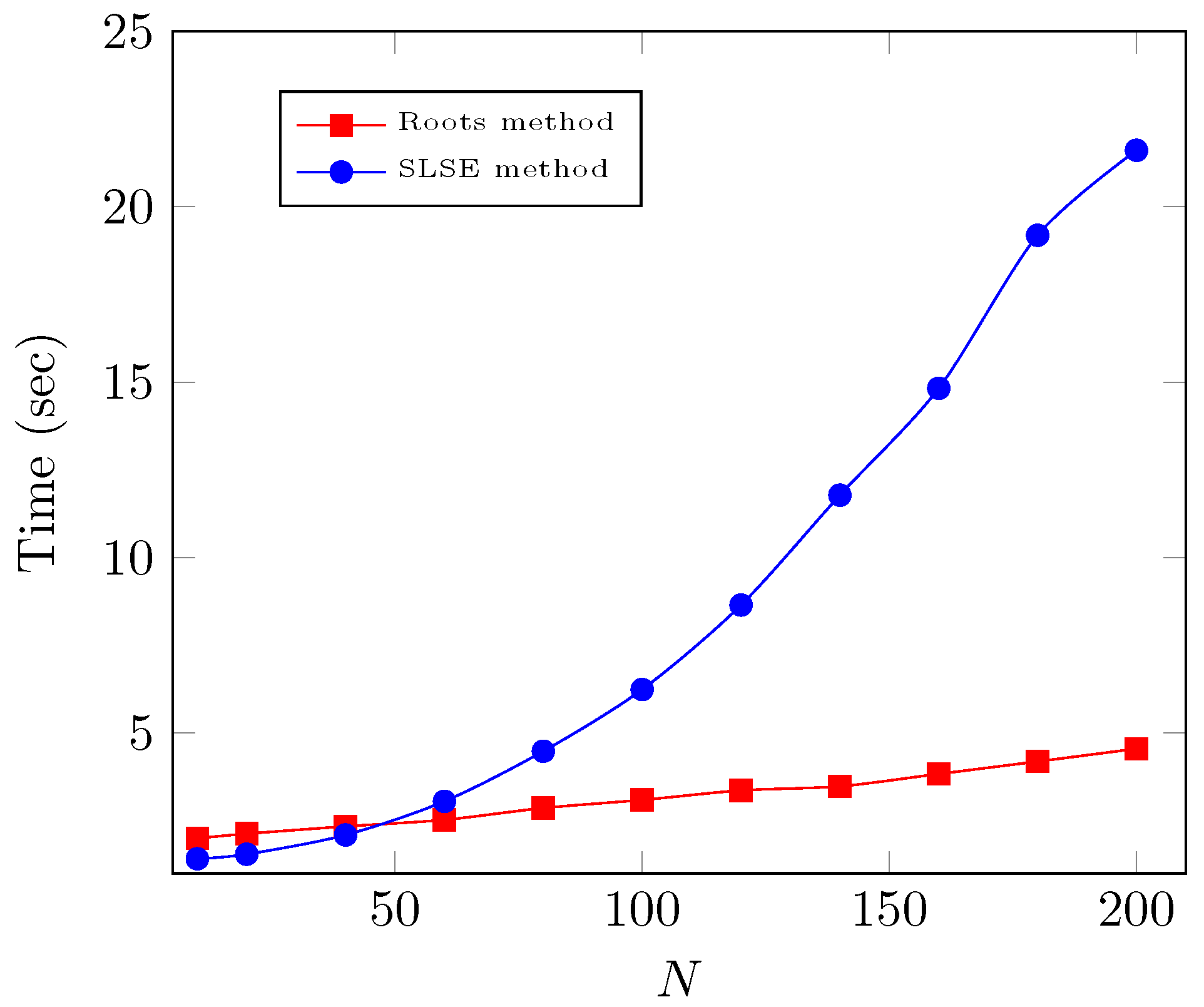
  • Finally, we compare the roots’ method against the process that uses simultaneous equations and present the results in the numerical section. It clearly shows that the roots approach takes less time.
The remaining paper is structured as follows. Section 2 specifies the model. Section 3 analyzes the G e o / G a , Y / 1 / N system and finds queue-length distributions for the LAS-DA policy. Section 4 examines various system performance measurements. Section 5 provides some numerical results and, finally, the paper is concluded in Section 6.
Remark 1.
It may be useful to comment on the matrix-analytic and the root-finding method. Kendall [19] made a famous remark that queueing theory wears the Laplacian curtain. Kleinrock [20] (p. 291) states, “One of the most difficult parts of this method of spectrum factorization is to solve for the roots”. Neuts (see Neuts’ book [21] and also Stidham [22]) states, “In discussing matrix-analytic solutions, I had pointed out that when the Rouché roots coincide or are close together, the method of roots could be numerically inaccurate. When I finally got copies of Crommelin’s papers, I was elated to read that, for the same reasons as I, he was concerned about the clustering of roots. In 1932, Crommelin knew; in 1980, many of my colleagues did not …”. Following this, several other researchers made similar comments. Given this, the procedure for solving queueing models led to the matrix-analytic or matrix-geometric method. In response, Chaudhry et al. [16] showed that the roots can be found even when the number involved is large. (This was done when MATHEMATICA OR MAPLE failed to give those roots. We can now use this software to find roots.)

2. Model Description

We consider a G e o / G a , Y / 1 / N queue where jobs arrive following a Bernoulli process with parameter λ . A single server processes the jobs on a first-come-first-served (FCFS) discipline in batches with a random capacity Y possessing a probability mass function (pmf) P ( Y = i ) = y i , i = a , a + 1 , , b with i = a b y i = 1 , the probability generating function (PGF) Y ( z ) = i = a b y i z i , mean E ( Y ) = i = a b i y i and Y ( z ) = z b Y ( z 1 ) . We assume the minimum and maximum threshold values of the random variable Y as a and b, respectively. When there are at least a jobs in the queue, the server commences serving a batch of size i with probability y i (when there are Y b , it takes all of them). When the number of jobs comes down below a threshold value a ( 1 ) in the system, the server remains idle but awaits the number of jobs to rise to a; when it attains a, it resumes service. The service times { S n , n 1 } are independently and identically distributed (iid) with arbitrary pmf s k = P ( S n = k ) , k = 1 , 2 , and s 0 = 0 , the PGF S ( z ) = i = 1 s i z i and mean service time E ( S ) = s = d d z S ( z ) | z = 1 = 1 / μ .
The processing times of the jobs are independent of the arrival process and the number of jobs served. The waiting buffer has a finite capacity N with b N . Thus, in the system, no more than N + b jobs can be available anytime. We presume offered load of the system as ρ = λ E ( S ) / E ( Y ) . In LAS-DA policy, arrivals occur in ( u , u ) , and departures take place in ( u , u + ) ; arrivals supersede departures. Figure 1 describes the various time periods at which events occur. For more details on this, one may refer to [5,6].

3. Queue-Length Distributions

Here, we find steady-state queue-length distributions at various epochs of G e o / G a , Y / 1 / N queue with the LAS-DA policy.

3.1. Post-Departure Epoch Probabilities

Let Q + be the number of jobs in the queue after completing the th service. Suppose A + 1 and Y + 1 represent the number of arrivals throughout the processing time on the ( + 1 ) th job and the processing capacity of ( + 1 ) th service, respectively. As per the batch service rule, the departure epoch queue lengthis
Q + 1 + = min Q + Y + 1 + + A + 1 , N ,
where x + = max ( x , 0 ) . The probability distribution of A + 1 is
k n = P ( A + 1 = n ) = j = 1 P A + 1 = n | S + 1 = j P S + 1 = j = j = n s j j n λ n ( 1 λ ) j n , n 0 .
Here we may note that arrivals are generated by a Bernoulli sequence by the property of geometric interarrival times. In LAS-DA, if the service time of the ( + 1 ) th job is j slots, then there will be j time slots where n arrivals may occur. One may note that j n λ n ( 1 λ ) j n is the probability of n arrivals in j slots. Let K ( z ) = n = 0 k n z n be the probability generating function of the sequence { k n , n = 0 , 1 , } . Thus
K ( z ) = n = 0 j = n s j j n λ n ( 1 λ ) j n z n = j = 0 s j ( 1 λ + λ z ) j = S ( 1 λ + λ z ) .
Transition probabilities in one step of underlying Markov chain for p i j = lim P r { Q + 1 + = j | Q + = i } are given as
p i j = k j , 0 i a , 0 j N 1 , k j r = i b y r + r = a i 1 y r k j i + r , a + 1 i b 1 , i a 1 j N 1 , r = a b y r k j i + r , b i N , i b j N 1 , N , 0 i a , j = N , N r = i b y r + r = a i 1 y r N i + r , a + 1 i b 1 , j = N , r = a b y r N i + r , b i N , j = N ,
where j = r = j k r and k j with j < 0 defined to be zero, and which leads to the transition probability matrix P = ( p i j ) as
P = 0 1 j N 1 N 0 1 a a + 1 b b + 1 N ( k 0 k 1 k j k N 1 N k 0 k 1 k j k N 1 N k 0 k 1 k j k N 1 N k 0 r = a + 1 b y r k 1 r = a + 1 b y r k j r = a + 1 b y r k N 1 r = a + 1 b y r N r = a + 1 b y r + k 0 y a + k j 1 y a + k N 2 y a + N 1 y a k 0 y b r = b 1 b y r k 1 b + r r = a b y r k j b + r r = a b y r k N 1 b + r r = a b y r k N b + r 0 k 0 y b r = a b y r k j b + r 1 r = a b y r k N b + r 1 r = a b y r k N b + r 1 0 0 0 r = a b y r k j N + r r = a b y r k r 1 r = a b y r r ) .
The ( + 1 ) th batch service starts when there are a jobs in the queue, and the state changeover occurs from 0 i a 1 to 0 j N 1 . If the state changeover is from state i a to state 0 j N 1 , then there is a busy period between the leaving epoch of the th batch and the commencement of processing ( + 1 ) st batch. Let the steady-state probability p + = { P 0 + , P 1 + , , P n + , , P N + } represent jobs at departure epochs. Then, in steady-state, p + = p + P can be expressed as follows:
P j + = i = 0 a P i + k j + i = a + 1 b 1 P i + r = i b y r k j + i = a + 1 b 1 P i + r = a i 1 y r k j i + r + i = b N P i + r = a b y r k j i + r , 0 j N 1 ,
P N + = i = 0 a P i + N + i = a + 1 b 1 P i + r = i b y r N + i = a + 1 b 1 P i + r = a i 1 y r N i + r + i = b N P i + r = a b y r N i + r ,
where the normalization condition is j = 0 N P j + = 1 . It may be noted that Equation (3) is redundant and will not be considered in analysis hereafter. Specify PGF of P j + as P + ( z ) = j = 0 N P j + z j . Multiplying Equation (2) by z j and then adding overall j, we obtain
P + ( z ) = j = 0 N 1 k j z j i = 0 a P i + + j = 0 N 1 z j i = a + 1 b 1 P i + r = i b y r k j + j = 0 N 1 z j i = a + 1 b 1 P i + r = a i 1 y r k j i + r + j = 0 N 1 z j i = b N P i + r = a b y r k j i + r + P N + z N ,
P + ( z ) 1 K ( z ) Y 1 z = K ( z ) i = 0 a 1 P i + 1 z i Y 1 z + P N + z N + K ( z ) i = a b P i + r = i b y r z i r = i b y r z r i = a b y i j = i + 1 N P j + r = N j + a k r z r + j i i = 0 a 1 P i + + i = a b P i + r = i b y r j = N k j z j .
Simplifying the above equation, we get
P + ( z ) = K ( z ) i = 0 a 1 P i + z b z i Y ( z ) + i = a b 1 P i + r = i b y r z b z i r = i b y r z b r z b K ( z ) Y ( z ) + z N + b P N + i = a b y i j = i + 1 N P j + r = N j + a k r z r + j i N z b K ( z ) Y ( z ) z N + b i = 0 a 1 P i + + i = a b P i + r = i b y r j = N k j z j N z b K ( z ) Y ( z ) .
Only the first expression on the right side of the Equation (4) will add to the coefficient of z j , j = 0 , 1 , N . To the right of Equation (4), we ignore the second and third expressions, which consist of an output of z higher than N + b . These are not required as we want to compare the coefficients of z j for j N on both sides in Equation (4) to find P j + for j = 0 , 1 , , N . Let
P N + ( z ) = K ( z ) i = 0 a 1 P i + z b z i Y ( z ) + i = a b 1 P i + r = i b y r z b z i r = i b y r z b r z b K ( z ) Y ( z ) ,
which is equivalent to the PGF of an infinite buffer case. The function P N + ( z ) is fully determined once P i + , i = 0 , 1 , , b 1 are known. One may observe that when ρ < 1 , Equation (5) denotes the PGF of discrete-time infinite buffer G e o / G a , Y / 1 queue. We can calculate the probabilities for ρ 1 in the case of a finite buffer G e o / G a , Y / 1 / N queue.
Remark 2.
Using a = 1 , the model is reduced to G e o / G Y / 1 / N queue.
Remark 3.
Taking y 1 = 1 , y i = 0 , 2 i b and a = 1 , the model becomes G e o / G / 1 / N queue and Equation (5) establishes PGF as P N + ( z ) = P 0 + K ( z ) 1 z K ( z ) z , where K ( z ) = S ( 1 λ + λ z ) , which corresponds to the results of [23].
Remark 4.
Taking y b = 1 and y i = 0 , i b , the model is reduced to G e o / G ( a , b ) / 1 / N and Equation (5) establishes the PGF as P N + ( z ) = K ( z ) i = 0 b 1 P i + z b z i z b K ( z ) .
Intending to establish a unified method to solve the queueing system G e o / G a , Y / 1 / N , we obtain { P n + } 0 N from P + ( z ) by using the roots of characteristic equation and partial-fraction expansion. The literature on queueing systems shows that arrival/service-time distributions that possess the generating function as a rational function deal with the broad class of distributions see [24]. For this, we suppose that K ( z ) = S ( 1 λ + λ z ) as a rational function in z, specified by
K ( z ) = S ( 1 λ + λ z ) = f ( z ) g ( z ) ,
where f ( z ) and g ( z ) are polynomials of degree m and s, respectively, where m and s can have any value, e.g., m can be greater than s, e.g., see Example 3(ii). Thus, we have from Equation (5),
P N + ( z ) = f ( z ) i = 0 a 1 P i + z b z i Y ( z ) + i = a b 1 P i + r = i b y r z b z i r = i b y r z b r z b g ( z ) f ( z ) Y ( z ) .
The denominator of Equation (6) is a polynomial of degree b + s which when equated to zero has b + s roots inside, on, or outside the unit circle z = 1 , say, γ 1 = 1 , γ i ( i = 2 , 3 , , b + s ) .
Remark 5.
If the denominator z b g ( z ) f ( z ) Y ( z ) of Equation (6) = 0 obtains roots close to each other or repeated roots, we may obtain them by applying advanced software packages, for instance, MATHEMATICA or MAPLE. The MAPLE script for calculating repeated roots is exemplified below for Equation
u ( y ) = ( y 2 ) ( y 5 ) 2 ( y 7 ) 3 ( y 11 ) .
r e s t a r t : D i g i t s : = 10 : w i t h ( R o o t F i n d i n g ) : m : = y 2 y 5 2 y 7 3 y 11 ; A n a l y t i c ( u , y , r e = 1 . . 10 , i m = 2 . . 10 ) ; 7.00000000000000 , 7.00000000000000 , 7.00000000000000 , 5.00000000000000 , 5.00000000000000 , 2.00000000000000 , 11.00000000000000
According to Rouché’s theorem, the denominator of Equation (6) has b zeros say, γ i ( i = 1 , 2 , , b ) inside the unit circle. As P N + ( z ) converges in z 1 , the b zeros within the unit circle of the denominator should cancel with the b zeros of the numerator. After canceling the b factors in the numerator and denominator, we can re-write Equation (6) as
P N + ( z ) = T C ( z ) + f 1 ( z ) i = b + 1 b + s ( z γ i ) ,
where C ( z ) = i = 0 n 0 c i z i and T is a normalizing constant. Note that when 2 m < s , then C ( z ) will be zero. In the partial-fraction process, a slight modification is needed ([25], p. 221) when all the roots are not distinct. Since we are looking at the finite buffer queue system, three instances appear here.
  • If ρ < 1 the s roots γ i , i = b + 1 , b + 2 , , b + s remain outside the circle z = 1 .
  • If ρ = 1 , among the s roots, one root is 1 , and the other roots γ i , i = b + 2 , b + 3 , , b + s are outside the unit circle z = 1 .
  • If ρ > 1 , among s roots, one root is inside, say γ b + 1 and the other roots γ i , i = b + 2 , b + 3 , , b + s are outside, see [26]. One may note that when ρ > 0 increases, one positive real root comes closer to the origin from right to left.
The expression (7) is tractable for inversion. Applying partial-fraction expansion to Equation (7) yields
P N + ( z ) = T C ( z ) + i = b + 1 b + s M i z γ i ,
where
M i = f 1 ( γ i ) j = b + 1 , j i b + s ( γ i γ j ) .
Using Equation (8), we have
P n + = T c n + i = b + 1 b + s M i γ i n + 1 , if n = 0 , 1 , , n 0 , T i = b + 1 b + s M i γ i n + 1 , if n = n 0 + 1 , n 0 + 2 , , N .
Employing the normalization condition n = 0 N P n + = 1 , we obtain the only unknown T as
T = i = 0 n 0 c i i = b + 1 b + s M i γ i × 1 γ i ( N + 1 ) 1 γ i 1 1 , if ρ 1 , i = 0 n 0 c i M b + 1 ( N + 1 ) i = b + 2 b + s M i ψ i × 1 ψ i ( N + 1 ) 1 ψ i 1 1 , if ρ = 1 .
Thus, once all the roots are known, we can get the distribution for the number in queue.
Remark 6.
It may be noted that it is also possible to find the probabilities { P n + } 0 N by assuming the solution of the form P j + = C z j , where C 0 . Unfortunately, if we use this method, we have to solve for N simultaneous equations.

3.2. Relationship between the Queue-Length Distributions at Post-Departure and Random Epochs

This sub-section establishes associations between probability at random and post-departure epochs by basic probabilistic reasoning and discrete-time renewal theory. In steady-state, let { P j } 0 N and { P j } 0 N be the probabilities representing the number of jobs in the queue at random times and before arrival, respectively. Since the inter-arrival times use geometric distribution, the arrivals are independent of other events. Thus, it implies that P j = P j , j = 0 , 1 , , N ; for details, see Boxma and Groenendijk [27]. If the server is idle, there are < a jobs in the queue. Suppose N q is the number of tasks in the queue at some random time. At a random epoch, the steady-state probabilities are P n , 0 = P ( N q = n , server   idle ) , 0 n a 1 , and P n , 1 = P ( N q = n , server   busy ) , 0 n N . Given this,
P j = P j , 0 + P j , 1 if   0 j a 1 P j , 1 if   a j N
Let the limiting pmf of the elapsed service time be s ^ , which is determined by s ^ = μ r = + 1 s r , 0 (see, [5] (p. 20)), and k ^ be the probability that the number of arrivals during an elapsed service time is . This yields
k ^ = i = i λ ( 1 λ ) i s ^ i , = 0 , 1 ,
If E * is the mean inter-departure time of processing batches, 1 / E * represents the departure rate. At the batch departure epoch, if the number of jobs in the queue is less than a, the subsequent batch departure occurs after an idle time and the service time processing time. Otherwise, the release of the next batch takes place following the processing time of the subsequent batch. This gives,
E * = E ( S ) 1 i = 0 a 1 P i + + i = 0 a 1 P i + a i λ + E ( S ) = E ( S ) + i = 0 a 1 P i + ( a i ) λ .
Remark 7.
It can also be put down as E * = E ( S ) + i = 1 a P a i + i λ . When a = 1 , it matches with Chaudhry and Chang [7].
Theorem 1.
The random- and post-departure-epoch probabilities { { P j , 0 } 0 a 1 , { P j , 1 } 0 N } , and { P j + } 0 N are related by
P j , 0 = i = 0 j P i + i = 0 a 1 ( a i ) P i + + λ E ( S ) , 0 j a 1 ,
P j , 1 = 1 i = 0 a 1 P i , 0 · [ i = 0 a 1 P i + k ^ j + i = a b 1 P i + m = i b y m k ^ j + i = a + 1 b 1 P i + m = a i 1 y m k ^ j i + m + i = b N P i + m = a b y m k ^ j i + m ] , 0 j N 1 .
Finally, P N , 1 can be found from P N , 1 = 1 j = 0 a 1 P j , 0 j = 0 N 1 P j , 1 .
Proof. 
The fraction of the time the batch server remains idle between two successive departure epochs is the probability of getting the server idle at a random epoch ( P i d l e ). Let E ( I ) be the mean idle period. Using the definition of E ( S ) and E ( I ) , we have
P i d l e = E ( I ) E ( I ) + E ( S ) , P j , 0 = P i d l e × P ( fraction   of   idle   perio ) = E ( I ) E ( I ) + E ( S ) × 1 λ i = 0 j P i + E ( I ) , 0 j a 1 ,
where E ( I ) = 1 λ i = 0 a 1 P i + ( a i ) . We employ system state conditioning and discreet renewal theory to find P j , 1 . The processor is active with probability ( 1 i = 0 a 1 P i , 0 ) ; thus,
P j , 1 = P ( N q = j , processor   active ) = ( 1 i = 0 a 1 P i , 0 ) P ( N q = j | processor   active )
Assuming that k j e is the number of jobs that come following an embedded Markov point until the elapsed service time, we have
P ( N q = j | processor   activ ) = i = 0 a 1 P i + m = a b y m k ^ j + i = a b 1 P i + m = i b y m k ^ j + i = a + 1 b 1 P i + m = a i 1 y m k ^ j i + m + i = b N P i + m = a b y m k ^ j i + m , 0 j N 1 .
Putting together (13) and (14), we obtain (12). We can obtain P N , 1 using normalization condition. Thus, we obtain random epoch probabilities { { P j , 0 } 0 a 1 , { P j , 1 } 0 N } in connection with post departure epoch probabilities { P j + } 0 N . □
Though the relations between random- and post-departure epoch probabilities are available in [13] using transition rates, here, we develop an alternative method to obtain the queue-length distributions at random epochs.
Because of BASTA (Bernoulli arrivals see time averages) property, see [5], the queue-length distribution exactly before arrival of job will be equal to that of P j , 0 and P j , 1 . Further, since the outside observation epoch falls in an interval between arrival and departure epochs, the outside observer’s distribution is the same as the random epoch distribution.

4. Performance Measures

This section deals with several measures of performance. The average number of jobs in the queue ( L q ) is given by
L q = j = 0 a 1 j P j , 0 + j = 0 N j P j , 1
The probability of the processor being busy (PB) at some random moment is specified by 1 j = 0 a 1 P j , 0 . Due to the BASTA property, the loss or blocking probability ( P B L ) is given by P B L = P N , 1 . Since the effective arrival rate λ e = λ ( 1 P N , 1 ) , we can obtain the average wait time in the queue ( W q ) by employing Little’s law as W q = L q λ e . The reported result of W q in [13] is incorrect. They have applied the effective arrival rate as λ instead of λ e .
Remark 8.
If ρ < 1 and N , then λ e = λ and L q = j = 0 a 1 j P j , 0 + j = 0 j P j , 1 . Using Little’s law, the average waiting time in the queue ( W q ) can be computed as W q = L q λ .

5. Numerical Results

To exemplify the analytic results found in this article, we illustrate several numerical outcomes in tables and figures. We also give several performance measures, for instance, the average queue length ( L q ), the average waiting time in the queue ( W q ), and the probability of loss ( P l o s s ). The computations were performed in double precision and executed in a 64-bit windows 10 professional OS possessing Intel(R) corei5-6200U processor @ 2.30 GHz and 8 GB DDR3 RAM utilizing MAPLE 18 software. The numerical results were exact, but we reported outcomes rounding to six decimal places. Because reported outcomes are rounded, the sum of probabilities may not add up to one in some cases.
Example 1.
G e o / N B 2 a , Y / 1 / 10 queue. Consider the distribution of service time as being in two stage negative binomial distribution (NB) with PGF S ( z ) = μ z 1 μ ¯ z 2 . Here, we consider the same parameters as in Table 1 of the paper [13] to compare the results. The parameters are E ( S ) = 5 , y 2 = 0.2 , y 3 = 0.1 , y 4 = 0.7 , and E ( Y ) = 3.5 . The arrival rates are 0.14 , 0.35 , and 0.56 with corresponding traffic intensities ρ = 0.2 , 0.5 , and 0.8 , respectively. To show the evaluation process, let us assume λ = 0.14 . The denominator of Equation (6) has six roots, two of which are outside, and four are in and on the unit circle. From Equation (8),
P N + ( z ) = T 0.068061 + 7.817631 z 6.392624 6.204397 z 5.024572 ,
where T = 6.250001 . Similarly, the denominator of P N + ( z ) has two roots outside the unit circle when arrival rates are 0.35 and 0.56 , and we have from Equation (8),
P N + ( z ) = T c 0 + M b + 1 z γ b + 1 + M b + 2 z γ b + 2 ,
where γ b + 1 = 2.106094 , γ b + 2 = 3.454495 , T = 6.256038 , c 0 = 0.053212 , M b + 1 = 0.619857 , M b + 2 = 1.113392 and γ b + 1 = 1.304299 , γ b + 2 = 2.688401 , T = 6.867372 , c 0 = 0.025779 , M b + 1 = 0.081358 , M b + 2 = 0.224798 , respectively.
Now, we can find post-departure epoch probabilities from Equation (9). The results are presented in Table 1. We note that the results of queue-length distribution at post-departure epoch match the results given by Yi et al. [13], but the random epoch does not. We have also computed queue-length distributions at random epochs using their method for checking purposes. They match perfectly with our results. However, the results presented in the paper by [13] are different. Thus, various performance measures are also not the same.
Remark 9.
It may be noted that P N + ( z ) is a polynomial in both cases, as can be seen in Table 1. The same applies to other cases as well.
Example 2.
G e o / D P H a , Y / 1 / N queue. The service-time distribution is assumed to be discrete phase-type (DPH) having s k = α T k 1 T 0 , k = 1 , 2 , , T 0 = e T e , where e is the appropriate column vector with all elements equal in size. This gives the PGF of service-time distribution as S ( z ) = z α ( I zT ) 1 T 0 , | z | 1 . Table 2 shows the queue length distributions at different times employing the DPH service time distribution. For the first example of Table 2, we suppose
α = 0.40 0.50 0.10 ,   T = 0.10 0.20 0.05 0.30 0.15 0.10 0.20 0.50 0.10 ,
with E ( S ) = 2.005267 and the other parameters are λ = 0.7 , N = 15 , y 3 = 0.5 , y 5 = 0.3 , y 8 = 0.2 with E ( Y ) = 4.6 . Here the denominator of P N + ( z ) has eleven distinct roots, out of which three roots are outside the unit circle, and they are γ b + 1 = 2.254374 , γ b + 2 = 9.788249 , and γ b + 3 = 222.447161 . From Equation (8),
P N + ( z ) = T 3.63007 + 1.301912 z 2.254374 0.702111 z + 9.788249 + 930.333318 z + 222.447161 ,
where T = 1.755933 .
In the second example of Table 2, we assume α = 0.60 0.40 , and T = 0.5 1 / 3 1 / 3 1 / 3 with E ( S ) = 4.2 and the other parameters are λ = 0.84 , N = 50 , y 3 = 0.7 , y 4 = 0.2 , y 5 = 0.1 with E ( Y ) = 3.4 . As ρ = 1.0376 , we have one root in the range ( 0 , 1 ) from the remaining four roots, and the other three are outside the circle of unity. From Equation (8),
P N + ( z ) = T 0.000674 + 5.2 × 10 21 z 1.375407 + 0.001238 z 0.974373 0.006324 z 16.101113 4.900051 × 10 13 z 16.100784 ,
where T = 7.569441 .
Remark 10.
It may be noted that Equations (15) and (16) are polynomials since the coefficients of z b are zero. This may be seen in Table 1. This also applies to all the examples that follow.
Example 3.
As before, in this example, we consider two cases: (i) G e o / M G e o 2 2 , Y / 1 / 10 queue. Here, the service time is a mixture of two geometric distributions with PGF S ( z ) = ς 1 μ 1 z 1 ( 1 μ 1 ) z + ς 2 μ 2 z 1 ( 1 μ 2 ) z , where ς 1 + ς 2 = 1 . The parameters are taken as E ( S ) = 2.83333 , N = 10 , ς 1 = 0.6 , μ 1 = 0.4 , μ 2 = 0.3 , y 2 = 0.2 , y 3 = 0.1 , y 4 = 0.7 , E ( Y ) = 3.5 , λ = 0.14 . The denominator of P N + ( z ) has six distinct roots, out of which two roots are outside the unit circle, and they are γ b + 1 = 4.031316 and γ b + 2 = 5.727647 . From Equation (8),
P N + ( z ) = T 0.561775 1.819848 z 4.031316 4.545280 z 5.727647 ,
where T = 1.0000001 .
(ii) G e o / D 2 , Y / 1 / 50 queue. Here, we consider service-time distribution as deterministic with PGF S ( z ) = z k for some constant k = 4 , s k = 1 . The parameters are taken as E ( S ) = 4 , N = 50 , y 2 = 0.5 , y 3 = 0.2 , y 4 = 0.1 , y 5 = 0.1 , y 6 = 0.1 , E ( Y ) = 3.1 , and λ = 0.4 . In this case, the denominator of P N + ( z ) has eight distinct roots, out of which two roots are outside the unit circle, and they are γ b + 1 = 5.019701 and γ b + 2 = 11.795711 . From Equation (8),
P N + ( z ) = T 1.316734 z 2 + 1.021799 z 102.664691 + 879.864750 z + 11.795711 141.482007 z 5.019701 ,
where T = 1 . Table 3 presents queue-length distributions at various epochs when the service-time distributions are a mixture of geometric and deterministic.
Example 4.
Here, we consider two cases. Table 4 presents the results of G e o / G a , Y / 1 / which can be found from the G e o / G a , Y / 1 / N system by assuming ρ < 1 and buffer capacity N appropriately large. We can easily compute the queue-length distributions of infinite queue capacity from finite queue capacity by assuming ρ < 1 and N sufficiently large.
(i) G e o / N B a , Y / 1 / queue. Here, we assume negative binomial (NB) service time distribution and the parameters are taken as λ = 0.703 , E ( S ) = 5 , y 2 = 0.5 , y 4 = 0.2 , y 5 = 0.1 , y 6 = 0.1 , y 8 = 0.1 with E ( Y ) = 3.7 . From Equation (8), we have
P N + ( z ) = T 0.005129 + 0.03006 z 2.520637 0.00745 z 1.042657 ,
where T = 6.250024 .
(ii) G e o / D P H a , Y / 1 / queue. For a DPH service time distribution, the settings are chosenas
α = 0.60 0.40   a n d   T = 0.5 1 / 3 1 / 3 1 / 3 .
with E ( S ) = 4.2 and the other parameters are λ = 0.58 , y 2 = 0.5 , y 3 = 0.3 , y 4 = 0.2 , and E ( Y ) = 2.7 . From Equation (8), we have
P N + ( z ) = T 0.001463 + 0.019982 z 22.872839 3.590919 × 10 14 z 22.870101 0.004169 z 1.080550 + 1.09 × 10 20 z 1.543692 ,
where T = 20.250 .
In Figure 2, we compare the processing times to calculate probabilities at post-departure using the proposed technique and the method used by [13] (solving a linear system of equations (SLSE)) against finite buffer capacity. We take the NB service-time distribution in two stages with the input parameters in the same way as in Table 1 for ρ = 0.2 . We notice that, with the increase of N, the time needed by the roots method remains almost static, whereas the method used by [13] takes more time for larger buffer size N and increases remarkably as N increases. In the roots method, the variation of the time is minimal. This is because of the initial estimation of the Newton iterative method for the calculation of polynomial roots. The application of the SLSE process is low in reliability and time-consuming. The root method provides a faster solution and superior performance in solving a linear system of method equations both in speed and reliability.
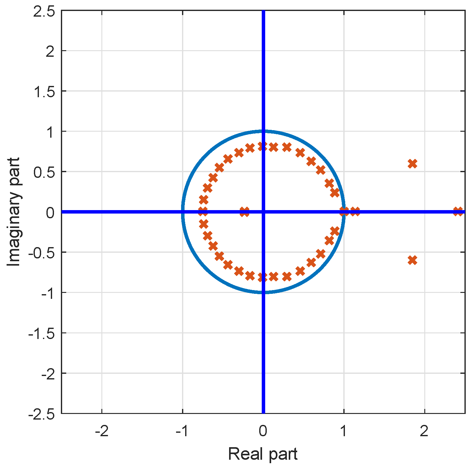
Figure 3 shows the roots of the characteristic equation for the number in the queue with NB service time distribution having 4 successes is the convolution of 4 geometric distributions. Here we consider the parameters as λ = 0.81 , y 4 = 0.4 , y 6 = 0.1 , y 12 = 0.1 , y 25 = 0.2 , y 30 = 0.1 , y 36 = 0.1 , and ρ = 0.54 . There are 40 of roots inside, on, and out of the unit circle for the assumed parameters. Here the characteristic equation is
z 36 0.886 + 0.486 z 4 0.0256 0.19 + 0.81 z 4 0.1 + 0.4 z 32 + 0.1 z 30 + 0.1 z 24 + 0.2 z 11 + 0.1 z 6 .

6. Conclusions

This article focuses on the G e o / G a , Y / 1 / N queue length distributions at various points in time. We use the roots of the associated characteristic equation to determine a unified way to compute performance measures for both infinite- and finite-buffer systems. Queue length distributions at a post-departure time are computed using an embedded Markov chain method. We obtain associations between queue length distributions at several time points by applying system state conditioning and discrete renewal theory. Several performance indices have been carried out, such as the blocking probability, the average wait time in the queue, and the average number of jobs in the queue. We illustrate them by using different numerical outcomes. The approach discussed in this paper can be used to cover cases when customers arrive in groups or even when arrivals are correlated (D-MAP-discrete Markovian arrival process).

Author Contributions

Conceptualization, M.C. and V.G.; methodology, V.G. and M.C.; Writing—original draft preparation, V.G.; supervision, M.C.; funding acquisition, M.C. All authors have read and agreed to the published version of the manuscript.

Funding

This research was funded by FMAS IO 757193 (C143).

Data Availability Statement

Not applicable.

Conflicts of Interest

The authors declare no conflict of interest.

Appendix A. The Continuous-Time Case

Here, we consider the relation between the discrete-time G e o / G a , Y / 1 / N queue and its continuous-time analogue. Let the time axis be divided into periods of uniform length Δ u with Δ u > 0 sufficiently small. In G e o / G a , Y / 1 / N , since the inter-arrival times ( u ) follow geometric distribution, the arrivals will follow binomial distribution which, as we have seen earlier, leads to PGF for binomial distribution. In the continuous-time case, geometric tends to exponential, and binomial tends to Poisson distribution, and the PGF tends to Laplace transform. Let us discuss this analytically. Assume that the inter-arrival times in the case of M / G a , Y / 1 / N have a rate α . Then, λ = α Δ u + o ( Δ u ) . In the discrete-case, let the service times S be in multiples of Δ u with probability P ( S = Δ u ) = s and = 1 s = 1 . Further, let n Δ u = v n , where the interval [ 0 , v n ] is divided into n intervals of length Δ u . The PGF of an arrival (or no arrival) in the interval ( v , v + 1 ) is ( 1 λ + λ z ) . If we denote the probability density function of service times by h ( · ) , then
P ( service   finishes   in ( u , u + Δ u ) | service   time > u ) = h ( u ) Δ u + o ( Δ u ) and s = h ( v ) Δ u + o ( Δ u ) .
When Δ 0 , the PGF S ( 1 λ + λ z ) changes to a Laplace transform. Using the definition of Lebesgue integration and taking the limit as Δ 0 and λ = α Δ , we have
lim Δ 0 K ( z ) = lim Δ 0 = 1 s ( 1 λ + λ z ) = h ¯ ( α α z ) .
The proof of the above is not discussed in detail here since the method applied can be found in [28]. Now, using λ = α Δ , K ( z ) = h ¯ ( α α z ) in (5) and taking the limit as Δ 0 , we have
P N + ( z ) = h ¯ ( α α z ) i = 0 a 1 P i + z b z i Y ( z ) + i = a b 1 P i + r = i b y r z b z i r = i b y r z b r z b h ¯ ( α α z ) Y ( z ) ,
the connections for M / G a , Y / 1 / N system. Taking a = 1 , we have
P N + ( z ) = h ¯ ( α α z ) i = 0 b 1 P i + z b r = i b y r z i r = i b y r z r z b h ¯ ( α α z ) Y ( z ) ,
which matcheswith [29].
Note that we cannot obtain results of discrete-time analogue from [29], that is, the converse is not true.

References

  1. Chaudhry, M.L.; Templeton, J.G.C. First Course in Bulk Queues; Wiley: New York, NY, USA, 1983. [Google Scholar]
  2. Medhi, J. Stochastic Models in Queueing Theory; Elsevier: Amsterdam, The Netherlands, 2002. [Google Scholar]
  3. Bruneel, H.; Kim, B.G. Discrete-Time Models for Communication Systems Including ATM; Springer Science & Business Media: New York, NY, USA, 2012; Volume 205. [Google Scholar]
  4. Hunter, J.J. Mathematical Techniques of Applied Probability: Discrete Time Models: Basic Theory; Academic Press: New York, NY, USA, 2014; Volume 1. [Google Scholar]
  5. Takagi, H. Queueing Analysis: Discrete-Time Systems; North Holland: Amsterdam, The Netherlands, 1993; Volume 3. [Google Scholar]
  6. Gravey, A.; Hébuterne, G. Simultaneity in discrete-time single server queues with bernoulli inputs. Perform. Eval. 1992, 14, 123–131. [Google Scholar] [CrossRef]
  7. Chaudhry, M.L.; Chang, S.H. Analysis of the discrete-time bulk-service queue Geo/GY/1/N+ B. Oper. Res. Lett. 2004, 32, 355–363. [Google Scholar] [CrossRef]
  8. Denteneer, D.; Janssen, A.J.; Van Leeuwaarden, J. Moment inequalities for the discrete-time bulk service queue. Math. Methods Oper. Res. 2005, 61, 85–108. [Google Scholar] [CrossRef]
  9. Goswami, V.; Mohanty, J.; Samanta, S.K. Discrete-time bulk-service queues with accessible and non-accessible batches. Appl. Math. Comput. 2006, 182, 898–906. [Google Scholar] [CrossRef]
  10. Gupta, U.C.; Goswami, V. Performance analysis of finite buffer discrete-time queue with bulk service. Comput. Oper. Res. 2002, 29, 1331–1341. [Google Scholar] [CrossRef]
  11. Janssen, A.J.; VanLeeuwaarden, J. Analytic computation schemes for the discrete-time bulk service queue. Queueing Syst. 2005, 50, 141–163. [Google Scholar] [CrossRef]
  12. Sivasamy, R.; Pukazhenthi, N. A discrete time bulk service queue with accessible batch: Geo/NB(L,K)/1. Opsearch 2009, 46, 321–334. [Google Scholar] [CrossRef]
  13. Yi, X.W.; Kim, N.K.; Yoon, B.K.; Chae, K.C. Analysis of the queue-length distribution for the discrete-time batch-service Geo/Ga,Y/1/K queue. Eur. J. Oper. Res. 2007, 181, 787–792. [Google Scholar]
  14. Banerjee, A.; Gupta, U.; Goswami, V. Analysis of finite-buffer discrete-time batch-service queue with batch-size-dependent service. Comput. Ind. Eng. 2014, 75, 121–128. [Google Scholar]
  15. Zeng, Y.; Xia, C.H. Optimal bulking threshold of batch service queues. J. Appl. Probab. 2017, 54, 409–423. [Google Scholar]
  16. Chaudhry, M.L.; Harris, C.M.; Marchal, W.G. Robustness of rootfinding in single-server queueing models. ORSA J. Comput. 1990, 2, 273–286. [Google Scholar] [CrossRef]
  17. Gouweleeuw, F.N. A General Approach to Computing Loss Probabilities in Finite Buffer Queues. Ph.D. Thesis, Vrije Universiteit Amsterdam, Amsterdam, The Netherlands, 1996. [Google Scholar]
  18. Powell, W.B. Stochastic Delays in Transportation Terminals: New Results in the Theory and Application of Bulk Queues. Ph.D. Thesis, Massachusetts Institute of Technology, Cambridge, MA, USA, 1981. [Google Scholar]
  19. Kendall, D.G. Some recent work and further problems in the theory of queues. Theory Probab. Its Appl. 1964, 9, 1–13. [Google Scholar] [CrossRef]
  20. Kleinrock, L. Theory. In Queueing Systems; Wiley-Interscience: New York, NY, USA, 1975; Volume 1. [Google Scholar]
  21. Neuts, M.F. Matrix-Geometric Solutions in Stochastic Models: An Algorithmic Approach; Courier Corporation: Washington, DC, USA, 1994. [Google Scholar]
  22. Stidham, S., Jr. Applied Probability in Operations Research: A Retrospective; University of North Carolina, Department of Operations Research: Chapel Hill, NC, USA, 2001. [Google Scholar]
  23. Chaudhry, M.L.; Goswami, V. The queue Geo/G/1/N+ 1 revisited. Methodol. Comput. Appl. Probab. 2019, 21, 155–168. [Google Scholar] [CrossRef]
  24. Botta, R.F.; Harris, C.M.; Marchal, W.G. Characterizations of generalized hyperexponential distribution functions. Stoch. Model. 1987, 3, 115–148. [Google Scholar] [CrossRef]
  25. Kobayashi, H.; Mark, B.L.; Turin, W. Probability, Random Processes, and Statistical Analysis: Applications to Communications, Signal Processing, Queueing Theory and Mathematical Finance; Cambridge University Press: Cambridge, UK, 2011. [Google Scholar]
  26. Cohen, J.W. The Single Server Queue; North Holland Publising Company: Amsterdam, The Netherlands, 1982. [Google Scholar]
  27. Boxma, O.J.; Groenendijk, W.P. Waiting times in discrete-time cyclic-service systems. IEEE Trans. Commun. 1988, 36, 164–170. [Google Scholar] [CrossRef]
  28. Yang, T.; Li, H. On the steady-state queue size distribution of the discrete-time Geo/G/1 queue with repeated customers. Queueing Syst. 1995, 21, 199–215. [Google Scholar] [CrossRef]
  29. Singh, V. Finite waiting space bulk service system. J. Eng. Math. 1971, 5, 241–248. [Google Scholar] [CrossRef]
Figure 1. Various time epochs in LAS-DA.
Mathematics 10 03142 g001
Figure 2. Time (in seconds) needed to calculate post-departure probabilities.
Mathematics 10 03142 g002
Figure 3. The 40 roots of Equation (17) when NB service-time distribution.
Mathematics 10 03142 g003
Table 1. Queue-length distributions at various epochs for the G e o / N B 2 2 , Y / 1 / 10 queue.
P j + { P j , 0 , P j , 1 }
ρ = 0 . 2 ρ = 0 . 5 ρ = 0 . 8 ρ = 0 . 2 ρ = 0 . 5 ρ = 0 . 8
P 0 + 0.4997340.1577550.030728 P 0 , 0 0.2449910.0669600.010330
P 1 + 0.3403350.2904590.113199 P 1 , 0 0.4118380.1902460.048385
P 2 + 0.1186580.2460520.169892 P 0 , 1 0.2399890.3016160.170317
P 3 + 0.0315820.1481370.161190 P 1 , 1 0.0771890.2062500.172979
P 4 + 0.0075320.0793980.135131 P 2 , 1 0.0199650.1161850.148409
P 5 + 0.0016940.0403010.107666 P 3 , 1 0.0046940.0604540.119818
P 6 + 0.0003680.0199320.084302 P 4 , 1 0.0010470.0302230.093880
P 7 + 0.0000780.0096920.065970 P 5 , 1 0.0002260.0147620.071726
P 8 + 0.0000160.0045980.049310 P 6 , 1 0.0000480.0072470.059329
P 9 + 0.0000030.0021090.033773 P 7 , 1 0.0000100.0033790.041064
P 10 + 0.0000010.0015670.048838 P 8 , 1 0.0000020.0015600.027772
P 9 , 1 0.0000000.0006650.016418
P 10 , 1 0.0000000.0004520.019571
Sum1.0000001.0000001.000000Sum1.0000001.0000001.000000
L q 0.5487331.0950562.820867
W q 3.9195213.1301455.137817
P B L 0.0000000.0004520.019571
Table 2. Queue-length distributions at various epochs for the G e o / D P H 3 , Y / 1 / 15 and G e o / D P H 3 , Y / 1 / 50 queues.
G e o / D P H 3 , Y / 1 / 15 G e o / D P H 3 , Y / 1 / 50
y 3 = 0 . 5 , y 5 = 0 . 3 , y 8 = 0 . 2 y 3 = 0 . 7 , y 4 = 0 . 2 , y 5 = 0 . 1
λ = 0 . 7 , ρ = 0 . 30515 λ = 0 . 84 , ρ = 1 . 0376
j P j + P j , 0 P j , 1 j P j + P j , 0 P j , 1
00.1703940.0557660.25852300.0015370.0004320.009680
10.4699650.2095760.11194310.0096820.003150.009988
20.2006980.275260.04946420.0101140.0059890.010254
30.088375 0.02196330.010392 0.010524
40.039275 0.0097440.010666 0.010801
50.017414 0.00432150.010946 0.011085
100.000299 0.000074100.012463 0.012621
110.000133 0.000032200.016158 0.016363
120.000059 0.000014300.020947 0.021213
130.000026 0.000005400.027156 0.027501
140.000012 0.000001490.034304 0.009883
150.000005 0.000004500.035206 0.049366
Sum1.0000000.5406030.459397Sum1.0000000.0095700.990430
L q = 1.1208, W q = 1.6012 L q = 29.6650, W q = 7.1493
P B L = 0.000004 P B L = 0.049366
Table 3. Queue-length distributions at various epochs for the G e o / M G e o 2 2 , Y / 1 / 10 and G e o / D 2 , Y / 1 / 50 queues.
Geo / MGeo 2 2 , Y / 1 / 10 Geo / D 2 , Y / 1 / 50
y 2 = 0 . 2 , y 3 = 0 . 1 , y 4 = 0 . 7 y 2 = 0 . 5 , y 3 = 0 . 2 , y 4 = 0 . 1
μ 1 = 0 . 4 , μ 2 = 0 . 3 , ς 1 = 0 . 6 y 5 = 0 . 1 , y 6 = 0 . 1
λ = 0 . 14 , ρ = 0 . 11333 λ = 0 . 4 , ρ = 0 . 51613
j P j + P j , 0 P j , 1 j P j + P j , 0 P j , 1
00.6832220.3392970.1554900.1125800.0526500.353602
10.2505310.4637140.03249110.3130970.1990770.253667
20.051967 0.00699820.337945 0.107802
30.011114 0.00155130.177390 0.027021
40.002447 0.00035240.048246 0.004913
50.000553 0.00008250.008517 0.001019
60.000128 0.000019100.000003 0.000003
70.000030 0.000005200.000000 0.000000
80.000007 0.000001300.000000 0.000000
90.000002 0.000000400.000000 0.000000
100.000001 0.000000500.000000 0.000000
Sum1.0000000.8030100.196990Sum1.0000000.2517270.748273
L q = 0.516831, W q = 3.691651 L q = 0.775713, W q = 1.939284
P B L = 0.000000 P B L = 0.000000
Table 4. Queue-length distributions at various epochs when N .
Geo / NB 2 , Y / 1 / Geo / DPH 2 , Y / 1 /
y 2 = 0 . 5 , y 4 = 0 . 2 , y 5 = 0 . 1 , y 6 = 0 . 1 y 2 = 0 . 5 , y 3 = 0 . 3 , y 4 = 0 . 2 ,
y 8 = 0 . 1 , λ = 0 . 703 , ρ = 0 . 95 λ = 0 . 58 , ρ = 0 . 902
j P j + P j , 0 P j , 1 P j + P j , 0 P j , 1
00.0021770.0006160.0288740.0308090.0119920.070392
10.0132580.0043690.0348320.0715360.0398360.065422
20.029345 0.0362390.066885 0.060557
30.034741 0.0358800.061929 0.056044
40.035937 0.0348580.057314 0.051866
50.035505 0.0336090.053041 0.047999
100.029400 0.0273740.036007 0.032584
200.019366 0.0180280.016594 0.015016
300.012753 0.0118720.007647 0.006920
500.005531 0.0051490.001624 0.001470
1000.000685 0.0006380.000034 0.000031
1500.000085 0.0000790.000001 0.000001
2000.000011 0.0000100.000000 0.000000
2500.000001 0.0000010.000000 0.000000
3000.000000 0.0000000.000000 0.000000
5000.000000 0.0000000.000000 0.000000
Sum1.0000000.0049860.9950141.0000000.0518280.948172
L q =23.80989, W q =33.86898 L q =11.815062, W q =20.370796
Publisher’s Note: MDPI stays neutral with regard to jurisdictional claims in published maps and institutional affiliations.