The Discrete Fractional Variable-Order Tinkerbell Map: Chaos, 0–1 Test, and Entropy

Abstract

The dynamics of the Caputo-fractional variable-order difference form of the Tinkerbell map are studied. The phase portraits, bifurcation, and largest Lyapunov exponent (LLE) were employed to demonstrate the presence of chaos over a different fractional variable-order and establish the nature of the dynamics. In addition, the 0–1 test tool was used to detect chaos. Finally, the numerical results were confirmed using the approximate entropy.

1. Introduction

Nonlinear dissipative dynamical systems with at least one positive Lyapunov exponent, certain cross-product terms allowing dynamical effects between distinct state variables of the systems and all constrained system orbits are referred to as chaotic systems. Chaotic systems are investigated for being extraordinarily sensitive to little changes in their initial conditions [1]. An important feature of chaotic systems is their strange attractors; they are described by a fractal structure and a complex arrangement of points. Firstly, this chaotic behavior was seen in the dynamical systems with continuous time and it was considered to be an unfavorable characteristic. Researchers soon discovered that chaotic systems can also be discrete. In the examination of a meteorological model, a major revelation on chaos was made (Lorenz, 1963) [2]. The Lorenz system is an essential 3D chaotic system concept. Lorenz (1963) developed a system for describing chaotic systems, which has led to the discovery of certain 3D chaotic systems, such as the logistics map [3], Rössler map [4], 3D Stefanski systems [5], Hénon map [6], Lozi map [7], Sprott map [8], Chen system [9], and others.

Fractional calculus is an old mathematical concept that was created by mathematicians, such as Leibniz, Riemann, Liouville, and others [10]. However, it has not attracted much attention until the past few decades. Due to the complexity of its calculation and the ambiguity of its geometric importance, researchers discovered that fractional calculus can precisely explain several anomalous events, and it is now widely utilized to describe various mathematical issues in science and engineering [11,12,13,14,15]. The analysis of the dynamics of chaotic systems with fractional order has received a lot of attention, and significant results have been obtained. For instance, in [16], the dynamics of the discrete fractional Duffing system were analyzed; in [17], the dynamics, control, and synchronization of the fractional Ikeda map were investigated. However, even though the constant fractional calculus concept may handle certain significant physical issues, it is unable to capture significant kinds of physical events in which the order is a function of either dependent or independent variables. As a result, it implies that there are categories of physical problems that are better characterized by variable-order operators [18,19]. In [20], the authors introduced the first variable fractional order operator concept.

In 1993, S.G Samko and B. Ross studied operators with non-constant order derivatives or integrals. Finally, they investigated the notions of variable order derivatives and integrals when the orders of the fractional operators were feasible functions of time, space, etc. They also stated some of their characteristics. As a result, they developed the theory of fractional calculus, which has applications [21], such as in physics [22], signal processing [23], petroleum engineering [24], modeling of viscoelasticity oscillators [25], and mechanics [26]. Numerical solutions of a variable order fractional financial system are presented in [27]; in [28], the predator–prey model involving the variable order fractional differential equation with Mittag–Leffler kernel was analyzed. In [29], the authors studied the variable-order fractional chaotic maps: Chen’s map, logistic map, and Hénon map.

The chaotic discrete-time Tinkerbell map with the following formula is the subject of this study’s investigation:

$$\left\{\begin{array}{ccc}x(n+1)\hfill & =& x^2\left(n\right)-y^2\left(n\right)+\theta x\left(n\right)+\beta y\left(n\right),\hfill \\ y(n+1)\hfill & =& 2x\left(n\right)y\left(n\right)+\rho x\left(n\right)+\eta y\left(n\right),\hfill \end{array}\right.$$

(1)

where $\eta$, $\theta ,$$\rho$, and $\beta$ are parameters and n is the step of the discrete iteration.

The map’s name (1) is derived from the classic Cinderella narrative because the map’s path resembles Tinkerbell’s in the Disney film adaptation of the fictional story. Many researchers have investigated the Tinkerbell map because it includes many dynamics, such as a variety of periodic phases and chaotic behavior. For example, references [30,31,32,33] investigated its bifurcation under various situations and initial conditions. In [34], a more detailed investigation was carried out where the authors found factors that led to flip bifurcation, Hopf bifurcation, and fold bifurcation in the Tinkerbell map. In [35], the authors analyzed the dynamics of the Tinkerbell map with fractional order. The major purpose of this research was to improve the results obtained in [35] by using the Caputo-difference form of the Tinkerbell map with the fractional variable-order. The fractional variable-order form is likely to exhibit even more complex dynamics.

The research is organized as follows. Firstly, some definitions of discrete fractional calculus are presented. Then, the fractional variable-order Tinkerbell map is proposed. In addition, the dynamics of the proposed model along phase portraits, bifurcation, the largest Lyapunov exponent (LLE) diagrams, approximate entropy (ApEn), and the 0–1 test are analyzed. Finally, numerical simulations are executed to illustrate the obtained results.

2. Fractional Variable-Order Discrete-Time of the Tinkerbell Map

Before presenting the Tinkerbell map with the variable order, some essential theories according to the concept of the fractional calculus with discrete-time are given. In this paper, ${}^c{\Delta }_d^{\mu }v\left(r\right)$ represents the $\mu$-Caputo type delta difference of the function $v\left(r\right):{\mathbb{N}}_d\to \mathbb{R}$ with ${\mathbb{N}}_d=\left\{d,d+1,d+2...\right\}$ and $d\in \mathbb{R}$ fixed, which is defined as [36]:

$${}^c{\Delta }_d^{\mu }v\left(r\right)={\Delta }_d^{-(n-\mu )}{\Delta }^{n}v\left(r\right)=\frac{1}{\mathsf{\Gamma }(n-\mu )}\sum _{\sigma =d}^{r-(n-\mu )}{(r-\sigma -1)}^{(n-\mu -1)}{\Delta }^{n}v\left(\sigma \right),$$

(2)

for $\mu \notin \mathbb{N}$, where $r\in {\mathbb{N}}_{d+n-\mu }$ and $n=\left[\mu \right]+1$. The $\mu$-th fractional sum of $v\left(r\right)$ is given as [37]:

$${\Delta }_d^{-\mu }v\left(r\right)=\frac{1}{\mathsf{\Gamma }\left(\mu \right)}\sum _{\sigma =d}^{r-\mu }{(r-\sigma -1)}^{(\mu -1)}v\left(\sigma \right),$$

(3)

with $r\in {\mathbb{N}}_{d+\mu }$ and $\mu >0$. The term $r^{\left(\mu \right)}$ is the falling function, which is given by:

$$r^{\left(\mu \right)}=\frac{\mathsf{\Gamma }(r+1)}{\mathsf{\Gamma }\left(\omega \right)},$$

(4)

where $\omega$$=r+1-$$\mu$ and

$${\Delta }^{n}v\left(r\right)=\Delta \left({\Delta }^{n-1}v\left(r\right)\right)=\sum _{k=0}^n\left(\genfrac{}{}{0pt}{}{n}{k}\right){(-1)}^{n-k}v(r+k),r\in {\mathbf{N}}_d.$$

(5)

The standard forward difference operator, $\Delta v\left(r\right)=v(r+1)-v\left(r\right)$, is used to obtain the ’difference’ form of the system (1):

$$\left\{\begin{array}{ccc}\Delta x\left(n\right)\hfill & =& x^2\left(n\right)-y^2\left(n\right)+(\theta -1)x\left(n\right)+\beta y\left(n\right),\hfill \\ \Delta y\left(n\right)\hfill & =& 2x\left(n\right)y\left(n\right)+\rho x\left(n\right)+(\eta -1)y\left(n\right).\hfill \end{array}\right.$$

(6)

In the above system, when replacing n by $\omega =r-1+\mu$ and the difference operator $\Delta$ by the Caputo-like difference operator ${}^c{\Delta }_d^{\mu }$, the difference system with the fractional-order is obtained as:

$$\left\{\begin{array}{ccc}{}^c{\Delta }_d^{\mu }x\left(r\right)\hfill & =& x^2\left(\omega \right)-y^2\left(\omega \right)+(\theta -1)x\left(\omega \right)+\beta y\left(\omega \right),\hfill \\ {}^c{\Delta }_d^{\mu }y\left(r\right)\hfill & =& 2x\left(\omega \right)y\left(\omega \right)+\rho x\left(\omega \right)+(\eta -1)y\left(\omega \right),\hfill \end{array}\right.$$

(7)

where $r\in {\mathbb{N}}_{d+1-\mu }$, b is the starting point and $\mu \in ]0,1]$ is the fractional-order parameter. Now, replacing the Caputo-like difference operator ${}^c{\Delta }_d^{\mu }$ by the variable-order operator ${}^c{\Delta }_d^{\mu \left(r\right)}$, the fractional variable-order Tinkerbell map is given by:

$$\left\{\begin{array}{ccc}{}^c{\Delta }_d^{\mu \left(r\right)}x\left(r\right)\hfill & =& x^2\left(\omega \right)-y^2\left(\omega \right)+(\theta -1)x\left(\omega \right)+\beta y\left(\omega \right),\hfill \\ {}^c{\Delta }_d^{\mu \left(r\right)}y\left(r\right)\hfill & =& 2x\left(\omega \right)y\left(\omega \right)+\rho x\left(\omega \right)+(\eta -1)y\left(\omega \right),\hfill \end{array}\right.$$

(8)

where $r\in {\mathbb{N}}_{d+1-\mu \left(r\right)}$, $\mu \left(r\right)\in ]0,1]$, $\mu \left(r\right)$, and b are the variable order and the starting point, respectively.

3. Dynamics of the Tinkerbell Map with the Fractional Variable-Order

This section is devoted to numerical techniques for evaluating the dynamics of the suggested fractional Tinkerbell map with the variable-order (8). The discrete numerical formula is necessary to evaluate the solutions of the discrete Tinkerbell map with the fractional variable-order.

Now, the solution of the difference system fractional variable-order obtained in (8) is given by

$$\left\{\begin{array}{c}x\left(r\right)=x\left(d\right)+\frac{1}{\mathsf{\Gamma }\left(\mu \right(r\left)\right)}{\displaystyle \sum _{\sigma =d+1-\mu \left(r\right)}^{\sigma -\mu \left(r\right)}}{(r-\sigma -1)}^{\left(\mu \right(r)-1)}\{x^2(\sigma +\mu \left(r\right)-1)-y^2(\sigma +\mu \left(r\right)-1)\hfill \\ +(\theta -1)x(\sigma +\mu (r)-1)+\beta y(\sigma +\mu (r)-1)\},\hfill \\ y\left(r\right)=y\left(d\right)+\frac{1}{\mathsf{\Gamma }\left(\mu \right(r\left)\right)}{\displaystyle \sum _{\sigma =d+1-\mu \left(r\right)}^{\sigma -\mu \left(r\right)}}{(r-\sigma -1)}^{\left(\mu \right(r)-1)}\{2x(\sigma +\mu \left(r\right)-1)y(\sigma +\mu \left(r\right)-1)\hfill \\ +\rho x(\sigma +\mu (r)-1)+(\eta -1)y(\sigma +\mu (r)-1)\},\hfill \end{array}\right.$$

(9)

where $r\in {\mathbb{N}}_{d+1}$ (see [38]). As a result, since ${(r-\sigma -1)}^{\left(\mu \right(r)-1)}=\frac{\mathsf{\Gamma }(r-\sigma )}{\mathsf{\Gamma }(r-\sigma +1-\mu (r\left)\right)}$ and for $d=0$, the numerical formula is obtained by

$$\left\{\begin{array}{ccc}x\left(n\right)\hfill & =& x\left(0\right)+{\displaystyle \sum _{j=1}^n}\frac{\mathsf{\Gamma }(n-j+\mu (j\left)\right)}{\mathsf{\Gamma }\left(\mu \right(j\left)\right)\mathsf{\Gamma }(n-j+1)}\{x^2(j-1)-y^2(j-1)+(\theta -1)x(j-1)+\beta y(j-1)\},\hfill \\ y\left(n\right)\hfill & =& y\left(0\right)+{\displaystyle \sum _{j=1}^n}\frac{\mathsf{\Gamma }(n-j+\nu (j)}{\mathsf{\Gamma }\left(\mu \right(j\left)\right)\mathsf{\Gamma }(n-j+1)}\{2x(j-1)y(j-1)+\rho x(j-1)+(\eta -1)y(j-1)\}.\hfill \end{array}\right.$$

(10)

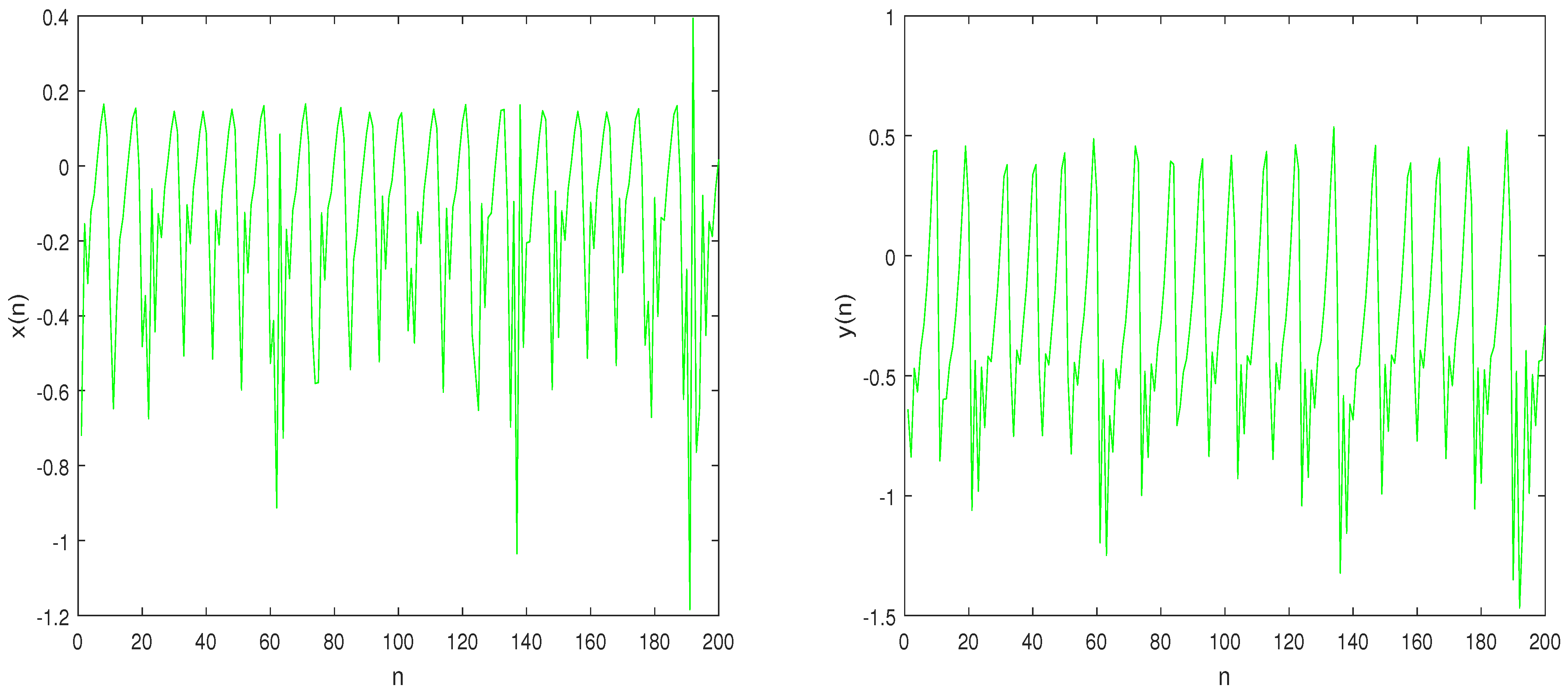
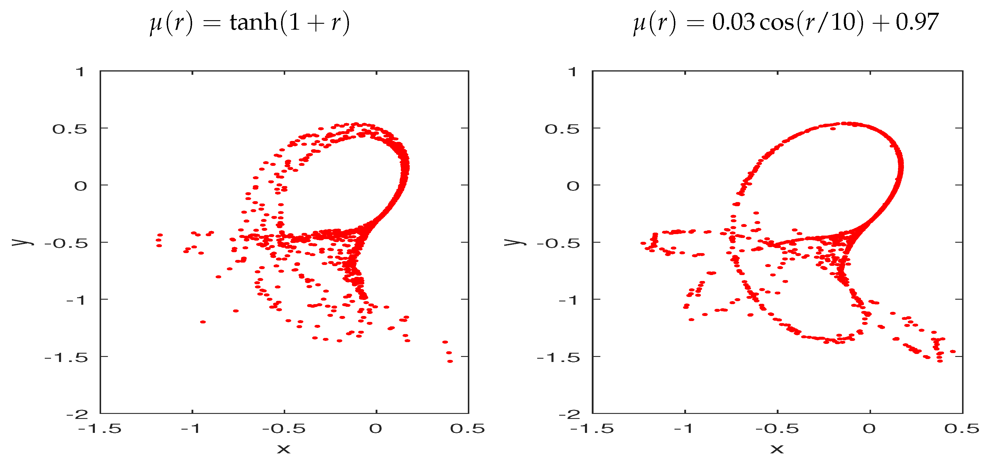
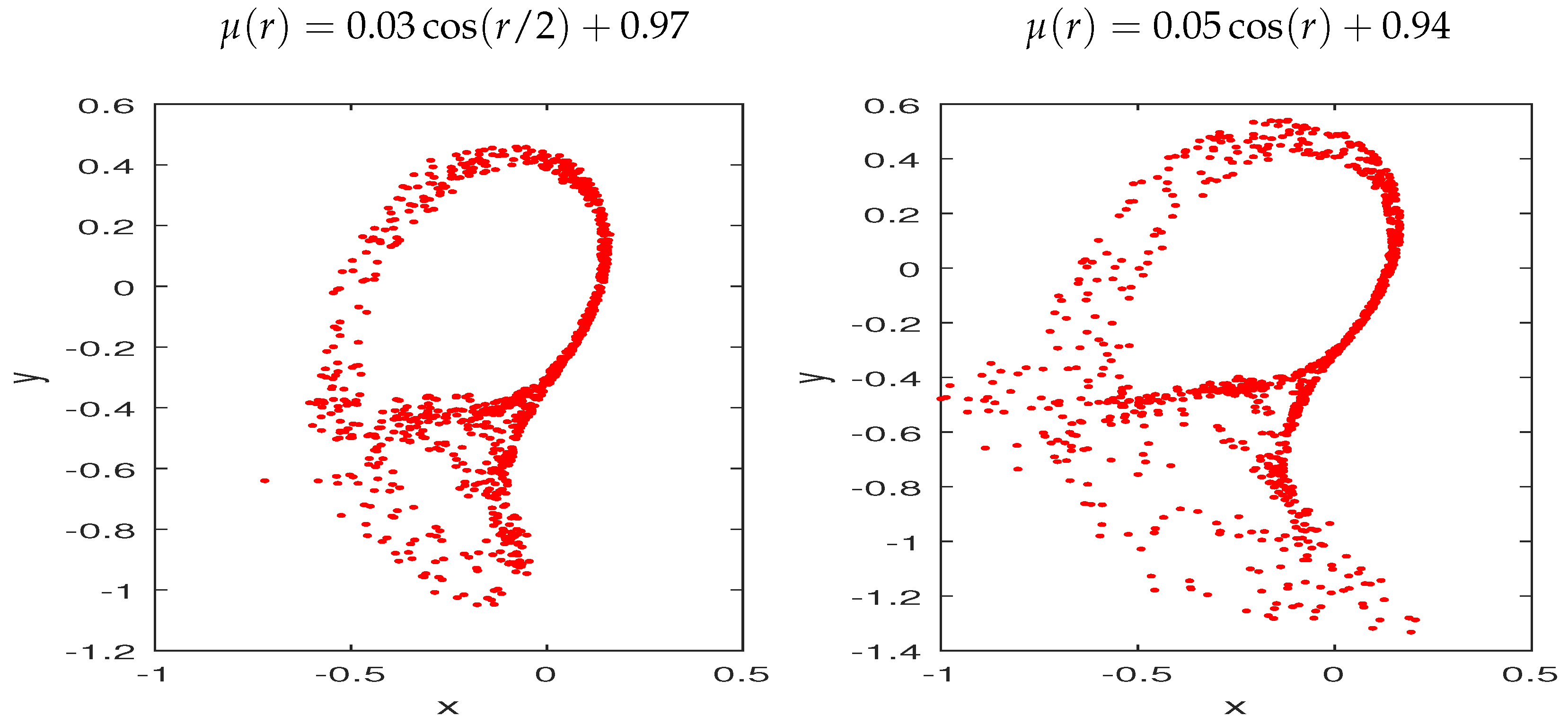
Now, the states of the fractional variable-order Tinkerbell map can be determined by using Formula (10); therefore, the plots of the bifurcation diagrams, time series of the states, and phase portraits can be obtained. The initial condition and parameters are taken from [35], i.e., $(\theta ,\beta ,\rho ,\eta )=(0.9,-0.6013,2,0.5)$ and $\left(x\right(0),y(0\left)\right)=(-0,72,-0.64)$. Figure 1 illustrates the time evolution of the states when $\mu \left(r\right)=0.03cos(r/10)+0.97$. It is more efficient to display the map’s trajectories in the state space because the discrete-time series in Figure 1 does not definitely demonstrate the absence or presence of chaos. Figure 2 displays the phase plots for several fractional variable-order functions: $\mu \left(r\right)=0.03cos(r/10)+0.97$, $\mu \left(r\right)=0.03cos(r/2)+0.97$, $\mu \left(r\right)=0.05cos\left(r\right)+0.94$ and $\mu \left(r\right)=tanh(1+r)$. One can see that the trajectory almost disappears when $\mu \left(r\right)=0.03cos(r/2)+0.97$, but the overall Tinkerbell shape remains valid for the other fractional variable-order functions.

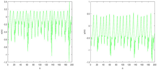
Figure 1. Time evolution of the system (8) states for the fractional variable-order $\mu \left(r\right)=0.03cos(r/10)+0.97$.

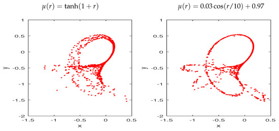
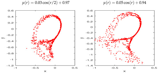
Figure 2. Phase portraits of the Tinkerbell map with fractional variable-order (8) with distinct fractional variable-orders.

Although phase portraits indicate the behavior of the map, a fuller view comes only after seeing the bifurcation of the map as a function of many parameters.

3.1. Bifurcation and Largest Lyapunov Exponents (LLE)

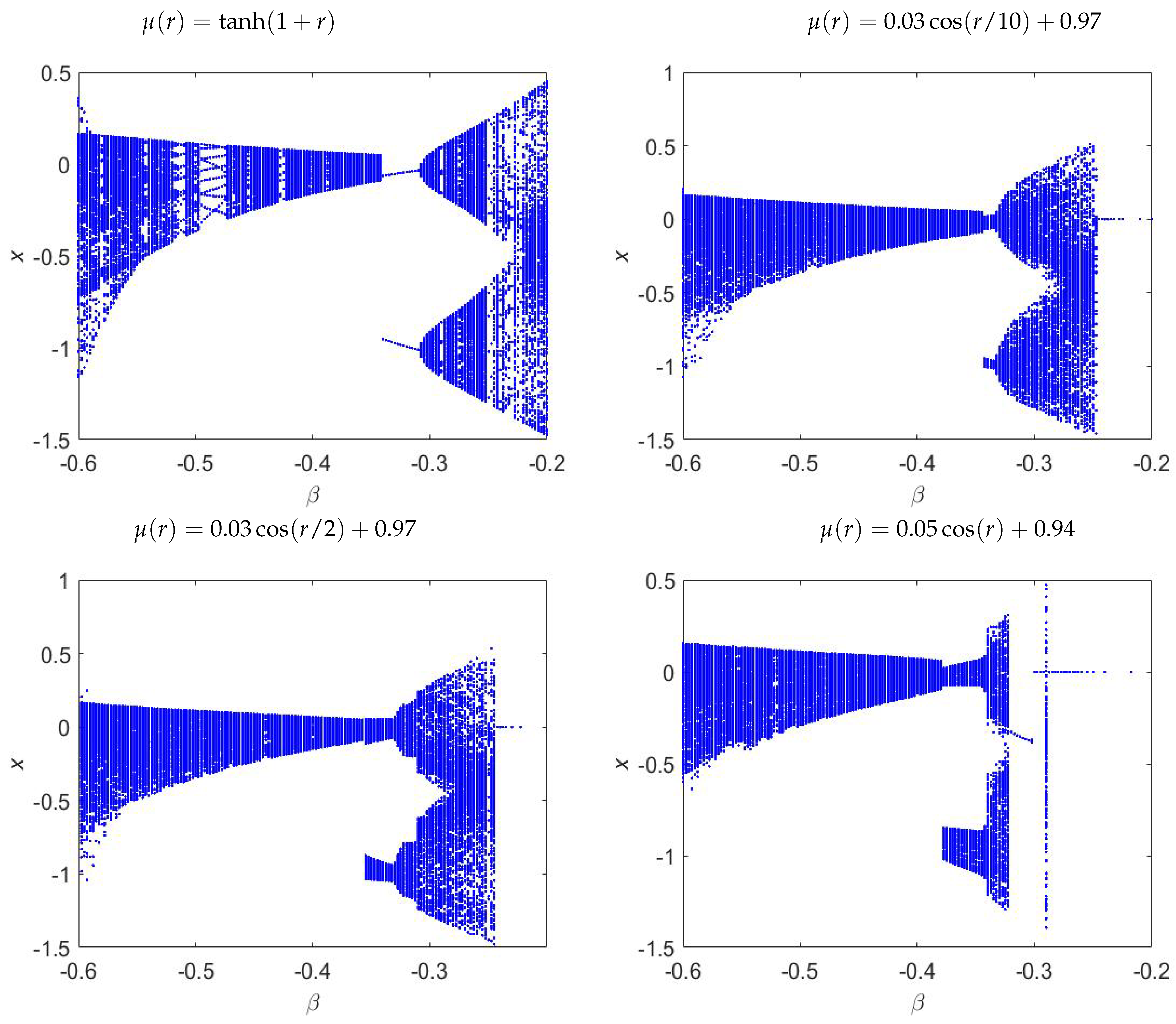
In this section, the bifurcation diagram and largest Lyapunov exponents are employed to study the dynamics of the Tinkerbell map with the fractional variable-order (8). Here, $\beta \in [-0.6,-0.2]$ is considered a critical parameter and $\Delta \beta =0.0025$. Figure 3 shows the bifurcation diagrams, which were derived using identical initial conditions and parameters as before. One can see that by considering the variable-order functions, the chaos exists for certain ranges of the parameter $\beta$. Although bifurcation diagrams are important in detecting the presence of chaos, the most useful tools are Lyapunov exponent(s) (LE). They can be calculated by using the Jacobian matrix method. The Lyapunov exponents are defined as [39]:

$$L{E}_k\left(x_0\right)=\underset{i\to \infty }{lim}\frac{1}{i}ln\mid {\lambda }_k^{\left(i\right)}\mid fork=1,2,$$

(11)

where ${\lambda }_k$ represent the eigenvalues of the matrix $J_i$ given by:

$$J_i=\left[\begin{array}{cc}{a}_i& b_i\\ c_i& d_i\end{array}\right],$$

(12)

where

$$a_i=a_0+\sum _{j=1}^n\frac{\mathsf{\Gamma }(n-j+\mu (j\left)\right)}{\mathsf{\Gamma }\left(\mu \right(j\left)\right)\mathsf{\Gamma }(n-j+1)}\{a_i(2x+\theta -1)+b_i(2y+\rho )\},$$

$$b_i=b_0+\sum _{j=1}^n\frac{\mathsf{\Gamma }(n-j+\mu (j\left)\right)}{\mathsf{\Gamma }\left(\mu \right(j\left)\right)\mathsf{\Gamma }(n-j+1)}\{a_i(\beta -2y)+b_i(2x+\eta -1)\},$$

$$c_i=c_0+\sum _{j=1}^n\frac{\mathsf{\Gamma }(n-j+\mu (j\left)\right)}{\mathsf{\Gamma }\left(\mu \right(j\left)\right)\mathsf{\Gamma }(n-j+1)}\{c_i(2x+\theta -1)+d_i(2y+\rho )\},$$

$$d_i=d_0+\sum _{j=1}^n\frac{\mathsf{\Gamma }(n-j+\mu (j\left)\right)}{\mathsf{\Gamma }\left(\mu \right(j\left)\right)\mathsf{\Gamma }(n-j+1)}\{c_i(\beta -2y)+d_i(2x+\eta -1)\},$$

and

$$\left[\begin{array}{cc}{a}_0& b_0\\ c_0& d_0\end{array}\right]=\left[\begin{array}{cc}1& 0\\ 0& 1\end{array}\right].$$

(13)

Figure 3. Bifurcation diagrams of the fractional variable-order Tinkerbell map (8) with $\beta \in [-0.6,-0.2]$ changed in steps of $\Delta \beta =0.0025$, parameters $(\theta ,\rho ,\eta )=(0.9,2,0.5)$, initial condition $\left(x\right(0),y(0\left)\right)=(-0.72,-0.64)$, and different fractional variable-orders.

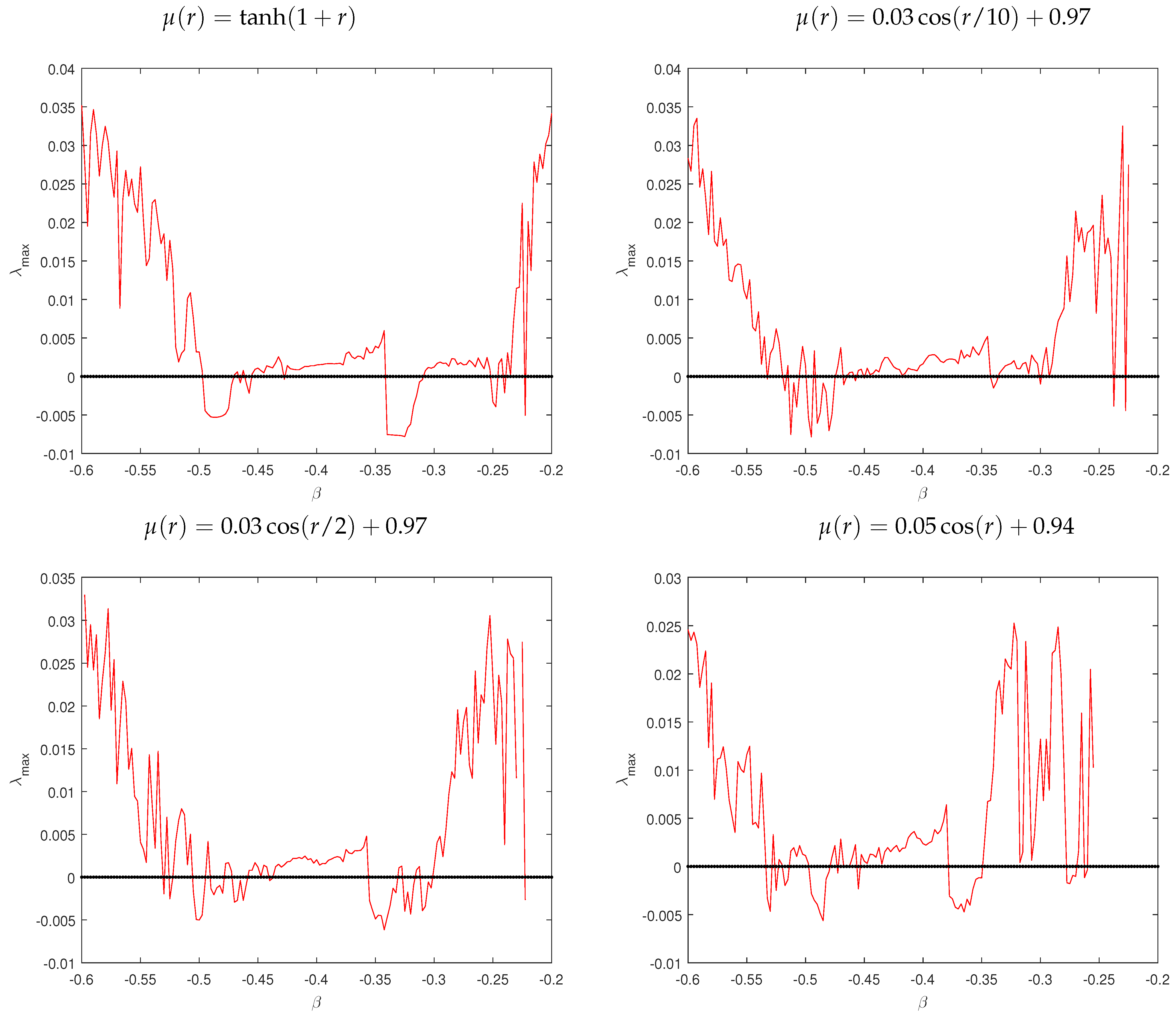
It is well known that when ${\lambda }_{max}$ is positive, the map is chaotic. Figure 4 illustrates the Lyapunov exponents with identical initial conditions, parameters, and fractional variable-order functions using the previous bifurcation plots (see Figure 3). Comparing the obtained results in Figure 3 and Figure 4, one can say that the (LLE) agrees well with the bifurcation diagrams.

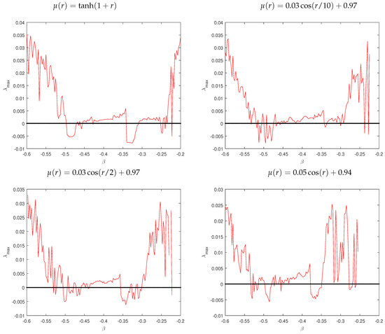
Figure 4. Plots of the largest Lyapunov exponents versus the parameter $\beta$ of the system (8) with distinct functions of the fractional variable-order.

3.2. The 0–1 Test

The 0–1 test tool [40] was used to analyze the dynamics of the Tinkerbell chaotic map with the fractional variable-order. The 0–1 test for chaos is another indicator, it was used to validate chaos from a time series. To represent this method, a set of states $\left\{u\right(l),l=1,2,\dots L\}$ was analyzed; the translation components p and q are given as:

$$p\left(l\right)=\sum _{i=1}^{l}u\left(i\right)\cos \left(ic\right),$$

(14)

$$q\left(l\right)=\sum _{i=1}^{l}u\left(i\right)\sin \left(ic\right),$$

(15)

where $l\in \{1,2,\dots L\}$ and c are chosen randomly in $(0,\pi )$.

By using p and q, the mean square displacement was determined by the following formula:

$$M_c=\frac{1}{L}\sum _{i=1}^L({(p(i+l)-p\left(i\right))}^2+{(q(i+l)-q\left(i\right))}^2),l<\frac{L}{10}.$$

(16)

The asymptotic growth rate was calculated by:

$$K_c=\underset{l\to \infty }{lim}\frac{log{M}_c}{logl}.$$

(17)

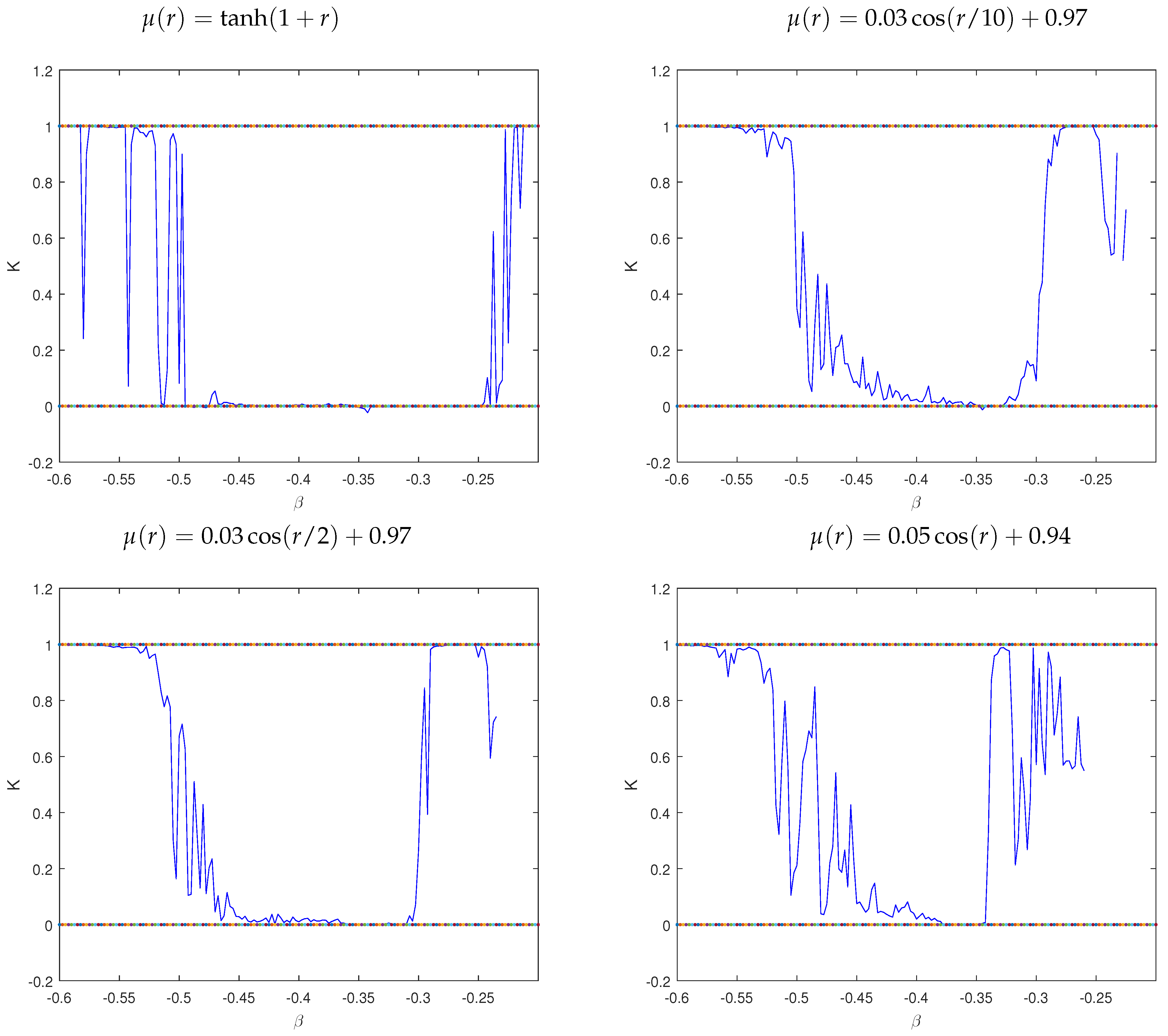
Thus, the system is chaotic when $K=median\left(K_c\right)$ approaches 1, and it is periodic when K approaches 0. Generally, if the system is regular, then the $p-q$ trajectories are bounded; when the $p-q$ trajectories are unbounded, the system is chaotic. To detect the chaotic behavior of the Tinkerbell map with the fractional variable-order, Figure 5 shows the asymptotic growth rate K with distinct fractional variable-orders and $p-q$ plots are depicted in Figure 6 and Figure 7. The state $u\left(l\right)$ is obtained by using identical initial conditions and parameters in Figure 3. In our results, the asymptotic growth rate K of the proposed map (8) approaches 1 for a specific range of $\beta$, which proves the existence of chaos. The results of the 0–1 test are consistent with the bifurcation and largest(LE) diagrams.

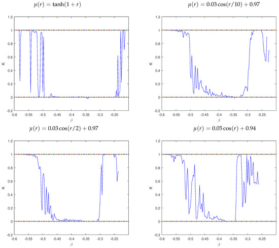
Figure 5. The 0–1 test plots of the Tinkerbell system with the fractional variable-order (8) for different fractional variable-orders.

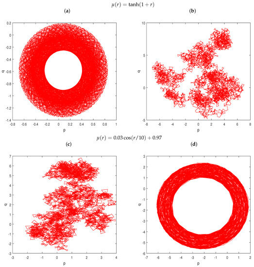
Figure 6. The p-q plots of the 0–1 test of the system (8) with different fractional variable-orders and values of $\beta$: (a) $\beta =-0.6013$, (b) $\beta =-0.30$, (c) $\beta =-0.58$, (d) $\beta =-0.31.$

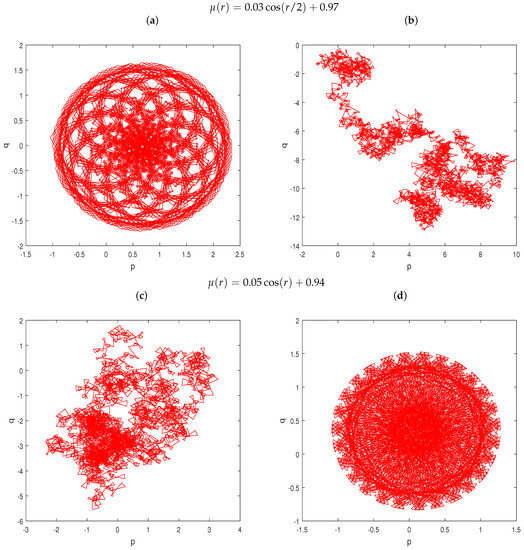
Figure 7. The p-q plots of the 0–1 test of the Tinkerbell map with the fractional variable-order (8) for distinct fractional variable-orders and values of $\beta$: (a) $\beta =-0.26$, (b) $\beta =-0.34$, (c) $\beta =-0.6013$, (d) $\beta =-0.37.$

3.3. The Approximate Entropy

Here, the complexity of the system (8) is described by using approximate entropy, which is defined as follows. (ApEn) assigns non-negative numbers where higher values show higher complexity. Let $w\left(1\right),w\left(2\right),\dots w\left(M\right)$ be a set of discrete states and present $M-m+1$ vectors by:

$$W\left(j\right)=\left[w\right(j),\dots w(j+m-1\left)\right].$$

(18)

The given vectors are the m consecutive w values, which begin with the jth state. Note that the value of the approximation entropy (ApEn) depends on two principal parameters: the tolerance r and the embedding dimension m. In this case, $r=0.2std\left(w\right)$ and $m=2$ where $std\left(w\right)$ presents the standard deviation of the data w. Define the following formula:

$$C_j^m\left(r\right)=\frac{k}{M-m+1},forj\in [1,M-m+1],$$

(19)

where k is the number of $W\left(j\right)$, which verifies the condition $d\left(W\right(j),W(l\left)\right)\le r$ and $d\left(W\right(j),W(l\left)\right)$ represents the distance between $W\left(j\right)$ and $W\left(l\right)$, the approximation entropy [41] is defined as:

$$ApEn={\chi }^m\left(r\right)-{\chi }^{m+1}\left(r\right),$$

(20)

where ${\chi }^m\left(r\right)$ is given by

$${\chi }^m\left(r\right)=\frac{1}{M-m-1}\sum _{j=1}^{M-m+1}log{C}_j^m\left(r\right).$$

(21)

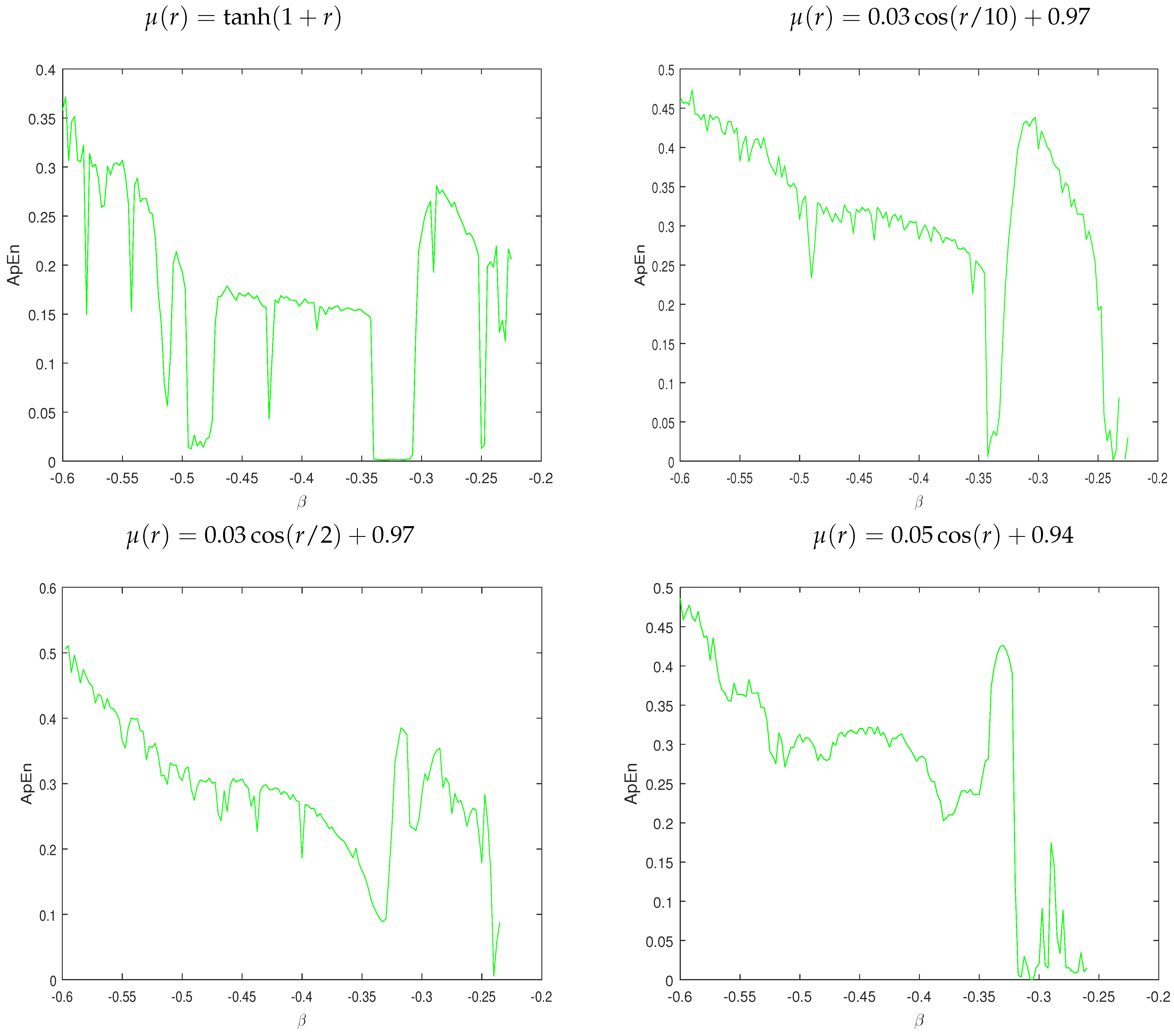
Figure 8 illustrates the approximate entropy (ApEn) of the proposed map (8) for several functions of the fractional variable-order.

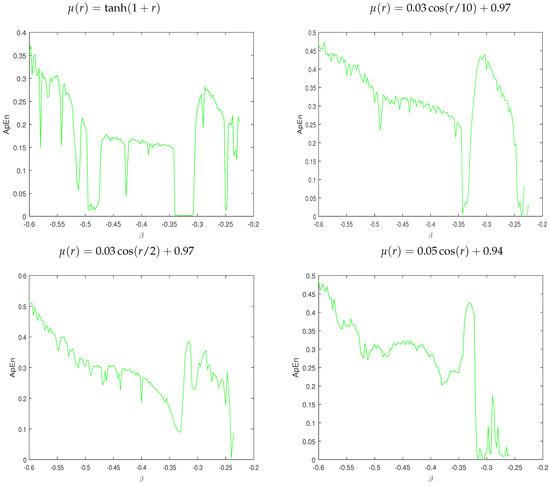
Figure 8. ApEn plots of the Tinkerbell map with the fractional variable-order (8) for several fractional variable-orders.

4. Conclusions and Future Works

In this research, the Caputo-difference form of the Tinkerbell map with fractional variable-order was studied. Phase-space portraits, bifurcation, and the largest Lyapunov exponent (LLE) indicate that the dynamics of the proposed system are dependent on the fractional variable-order. The 0–1 test and the approximation entropy (ApEn) confirmed our results obtained by the phase plots, bifurcation, and the largest Lyapunov exponent (LLE) diagrams. The results found in this work assure the successfulness of the fractional variable-order on the Tinkerbell map. One of the future goals is to use such systems and their applications in encryption and secure communications since the change of the fractional order to a fractional variable order makes the encryption more powerful.

References

- Vaidyanatham, S. Global chaos synchronisation of identical Li-Wu chaotic systems via sliding mode control. Int. J. Model. Identif. Control 2014, 22, 170–177. [Google Scholar] [CrossRef]
- Lorenz, E.N. Deterministic nonperiodic flow. J. Atmos. Sci. 1963, 20, 130–141. [Google Scholar] [CrossRef]
- May, R. Simple mathematical models with very complicated dynamics. Nature 1976, 261, 459–467. [Google Scholar] [CrossRef] [PubMed]
- Itoh, M.; Yang, T.; Chua, L.O. Conditions for impulsive synchronization of chaotic and hyperchaotic systems. Int. J. Bifurc. Chaos 2001, 11, 551–560. [Google Scholar] [CrossRef]
- Stefanski, K. Modelling chaos and hyperchaos with 3D maps. Chaos Solit. Fractals 1998, 9, 83–93. [Google Scholar] [CrossRef]
- Hénon, M. A two-dimensional mapping with a strange attractor. Commun. Math. Phys. 1976, 50, 69–77. [Google Scholar] [CrossRef]
- Lozi, R. Un atracteur étrange du type attracteur de Hénon. J. Phys. Colloq. 1978, 39, 9–10. [Google Scholar] [CrossRef]
- Sprott, J.C. Some simple chaotic flows. Phys. Rev. E 1994, 50, R647. [Google Scholar] [CrossRef]
- Chen, G.; Ueta, T. Yet another chaotic attractor. Int. J. Bifurc. Chaos 1999, 9, 1465–1466. [Google Scholar] [CrossRef]
- Hioual, A.; Ouannas, A. On fractional variable-order neural network with time varying external inputs. Innov. J. Math. 2022, 1, 52–65. [Google Scholar] [CrossRef]
- Kilbas, A.A.; Srivastava, H.M.; Trujillo, J.J. Theory and Applications of Fractional DiffErential Equations; Elsevier: Amsterdam, The Netherlands, 2006. [Google Scholar]
- Montesinos-García, J.J.; Martínez -Guerra, R. A numerical estimation of the fractional-order liouvillian systems and its application to secure communications. Int. J. Syst. Sci. 2019, 50, 791–806. [Google Scholar] [CrossRef]
- Magin, R.L. Fractional calculus in bioengineering. Begell House Redd. 2006, 2. [Google Scholar]
- Wang, L.; Song, Q. Pricing policies for dual-channel supply chain with green investment and sales effort under uncertain demand. Math. Comput. Simul. 2020, 171, 79–93. [Google Scholar] [CrossRef]
- Hilfer, R. Applications of Fractional Calculus in Physics; World Scientifc: Singapore, 2000. [Google Scholar]
- Ouannas, A.; Khennaoui, A.A.; Momani, S.; Pham, V. The Discrete Fractional Duffing System: Chaos, 0–1 Test, Co Complexity, Entropy and Control. Chaos 2020, 30, 083131. [Google Scholar] [CrossRef] [PubMed]
- Ouannas, A.; Khennaoui, A.A.; Odibat, Z.; Pham, V.T.; Grassi, G. On the dynamics, control and synchronization of fractional-order Ikeda map. Chaos Solitons Fractals 2019, 123, 108–115. [Google Scholar] [CrossRef]
- Sun, H.G.; Chen, W.; Chen, Y.Q. Variable-order fractional differential operators in anomalous diffusion modeling. Phys. A Stat Mech. Appl. 2009, 388, 4586–4592. [Google Scholar] [CrossRef]
- Coimbra, C.F.M. Mechanics with variable-order differential operators. Ann. Phys. 2003, 12, 692–703. [Google Scholar] [CrossRef]
- Samko, S.G.; Ross, B. Integration and differentiation to a variable fractional order. Integral Transform. Spec. Funct. 1993, 1, 277–300. [Google Scholar] [CrossRef]
- Yousefi, F.S.; Ordokhani, Y.; Yousefi, S. Numerical solution of variable order fractional differential equations by using shifted Legendre cardinal functions and Ritz method. Eng. Comput. 2020, 38, 1–8. [Google Scholar] [CrossRef]
- Pedro, H.T.C.; Kobayashi, M.H.; Pereira, J.M.C.; Coimbra, C.F.M. Variable order modeling of difusive-convective efects on the oscillatory fow past a sphere. J. Vib. Control 2008, 14, 1569–1672. [Google Scholar] [CrossRef]
- Sun, H.G.; Chen, Y.Q.; Chen, W. Random-order fractional differential equation models. Signal Process 2011, 91, 525–530. [Google Scholar] [CrossRef]
- Obembe, A.D.; Hossain, M.E.; Abu-Khamsin, S.A. Variable-order derivative time fractional difusion model for heterogeneous porous media. J. Petrol. Sci. Eng. 2017, 152, 391–405. [Google Scholar] [CrossRef]
- Soon, C.M.; Coimbra, C.F.M.; Kobayashi, M.H. The variable viscoelasticity oscillator. Ann. Phys. 2005, 14, 378–389. [Google Scholar] [CrossRef]
- Ingman, D.; Suzdalnitsky, J.; Zeifman, M. Constitutive dynamic-order model for nonlinear contact phenomena. J. Appl. Mech. 2000, 67, 383–390. [Google Scholar] [CrossRef]
- Ma, S.; Xu, Y.; Yue, W. Numerical solutions of a variable-order fractional financial system. J. Appl. Math. 2012, 2012, 417942. [Google Scholar] [CrossRef]
- Khan, A.; Alshahri, H.M.; Gómez-Aguilar, J.F.; Khan, Z.A.; Fernández-Anaya, G. A predator–prey model involving variable-order fractional differential equations with Mittag-Leffler kernel. Adv. Differ. Equ. 2021, 1, 1–18. [Google Scholar]
- Wu, G.C.; Deng, Z.G.; Beleanu, D.; Zeng, D.Q. New variable-order fractional chaotic systems for fast image encryption. Chaos 2019, 29, 083103. [Google Scholar] [CrossRef]
- Aulbach, B.; Colonius, F. Six Lectures on Dynamical Systems; World Scientific: Singapore, 1996. [Google Scholar]
- Nusse, H.; Yorke, J. Dynamics: Numerical Explorations; Springer: New York, NY, USA, 1997. [Google Scholar]
- Davidchack, R.; Lai, Y.; Klebanoff, A.; Bollt, E. Towards complete detection of unstable periodic orbits in chaotic systems. Phys. Lett. A 2001, 287, 99–104. [Google Scholar] [CrossRef]
- Mcsharry, P.; Ruffino, P. Asymptotic angular stability in non-linear systems: Rotation numbers and winding numbers. Dyn. Syst. 2003, 18, 191–200. [Google Scholar] [CrossRef]
- Yuan, S.; Jiang, T.; Jing, Z. Bifurcation and chaos in the tinkerbell map. Int. J. Bifurc. Chaos 2011, 21, 3137–3156. [Google Scholar] [CrossRef]
- Ouannas, A.; Khennaoui, A.A.; Bendoukha, S.; Vo, T.; Pham, V.; Huynh, V. The fractional form of the Tinkerbell map is chaotic. Appl. Sci. 2018, 8, 2640. [Google Scholar] [CrossRef]
- Abdeljawad, T. On Riemann and Caputo fractional differences. Comput. Math. Appl. 2011, 62, 1602–1611. [Google Scholar] [CrossRef] [Green Version]
- Atici, F.; Eloe, P.W. Discrete fractional calculus with the nabla operator. Electron. J. Qual. Theory Differ. Equ. 2009, 3, 1–12. [Google Scholar] [CrossRef]
- Chen, F.; Luo, X.; Zhou, Y. Existence results for nonlinear fractional difference equation. Adv. Differ. Equ. 2011, 2011, 713201. [Google Scholar] [CrossRef]
- Wu, G.C.; Baleanu, D. Jacobian matrix algorithm for Lyapunov exponents of the discrete fractional maps. Commun. Nonlinear. Sci. Numer. Simulat. 2015, 22, 95–100. [Google Scholar] [CrossRef]
- Gottwald, G.A.; Melbourne, I. A new test for chaos in deterministic systems. Proc. Math. Phys. Eng. Sci. 2004, 460, 603–611. [Google Scholar] [CrossRef]
- Pincus, S.M. Approximate entropy as a measure of system complexity. Proc. Natl. Acad. Sci. USA 1991, 88, 2297–2301. [Google Scholar] [CrossRef] [Green Version]
Publisher’s Note: MDPI stays neutral with regard to jurisdictional claims in published maps and institutional affiliations. |
© 2022 by the authors. Licensee MDPI, Basel, Switzerland. This article is an open access article distributed under the terms and conditions of the Creative Commons Attribution (CC BY) license (https://creativecommons.org/licenses/by/4.0/).