Article

Moore–Gibson–Thompson Photothermal Model with a Proportional Caputo Fractional Derivative for a Rotating Magneto-Thermoelastic Semiconducting Material

by
Osama Moaaz
1,*,
Ahmed E. Abouelregal
2,3,* and
Meshari Alesemi
4
1
Department of Mathematics, College of Science, Qassim University, P.O. Box 6644, Buraydah 51482, Saudi Arabia
2
Department of Mathematics, College of Science and Arts, Jouf University, Al-Qurayat 77455, Saudi Arabia
3
Department of Mathematics, Faculty of Science, Mansoura University, Mansoura 35516, Egypt
4
Department of Mathematics, College of Science, University of Bisha, Bisha 61922, Saudi Arabia
*
Authors to whom correspondence should be addressed.
Mathematics 2022, 10(17), 3087; https://doi.org/10.3390/math10173087
Submission received: 2 August 2022 / Revised: 13 August 2022 / Accepted: 23 August 2022 / Published: 27 August 2022

Abstract

:
By considering the Moore–Gibson–Thompson (MGT) equation, the current work introduces a modified fractional photothermal model. The construction model is based on the proportional Caputo fractional derivative, which is a new definition of the fractional derivative that is simple and works well. In addition, the theory of heat transfer in semiconductor materials was used in the context of optical excitation transfer and plasma processes. The proposed model was used to investigate the interaction of light and heat within a magnetized semiconductor sphere rotating at a constant angular speed. The Laplace transform was used to obtain solutions for optical excitation induced by physical field variables. Using a numerical method, Laplace transforms can be reversed. The figures show the effects of carrier lifetime, conformable fractional operator, and rotation on thermal and mechanical plasma waves, which are shown in the graphs. The theory’s predictions were compared and extensively tested against other existing models.

1. Introduction

Fractional calculus is the subfield of mathematical modeling that investigates and applies integrals and derivatives of non-integer order. The term “fractional” is erroneous, although it continues to be used since it is the most common term [1]. Over the past 30 years or more, several scientists have demonstrated a significant deal of interest in the topic of fractional calculus, which tackles derivatives and integrals of any order. In actuality, this interest was sparked by the significant results these experts gained when they applied this calculus’s tools to the analysis of real-world models [2,3,4]. Because not all real-world occurrences can be described using basic calculus operators, researchers attempted generalizations of these operators. It was discovered that fractional operators are good instruments for simulating long-memory processes as well as many phenomena seen in physical sciences, chemical engineering, electrical and mechanical design, as well as many other areas [5,6].
There are several derivatives and integrals in traditional fractional calculus, which is one of its strengths. However, there has always been a desire to refine calculus further and uncover new derivatives to comprehend the cosmos better. In addition, investigators required fractional operators other than Riemann–Liouville fractional operators to gain the best understanding and most accurate modeling of real-world issues. A few recently suggested fractional operators have non-singular kernels [7,8,9,10,11]. Studies previously suggested novel non-singular fractional operators because of the singularities found in standard fractional operators, which are expected to cause certain challenges in the modeling improvement. Exponentiation and the Mittag–Leffler functions appear in a number of these operators. Caputo and Fabrizio [7] developed a new non-singular fractional operator. Atangana and Baleanu [8] made their ideas work for a wider range of complex phenomena, including biological influences. Katugampola [12] presented what he termed extended fractional operators in order to combine the Riemann–Liouville and Hadamard fractional operators. The fractional derivatives of Caputo and Caputo–Hadamard were added to the generalized derivatives. Local derivatives allow differentiation and integration of orders that are not integers in other ways.
Jarad et al. [13] developed generalized RL and Caputo fractional derivatives with exponential functions in their kernels. In 2021, Baleanu et al. [14] presented new fractional operators mixing proportional and conventional integrals. Akgül and Baleanu [15] also looked into the analysis and testing of stabilization of the proportional Caputo derivative. Laplace transforms were utilized in these situations to explain how the symmetrical fractional derivatives were related in Riemann–Liouville and Caputo situations. The novel fractional operator in the Caputo sense is a generalization of the classical proportional derivative presented in [15], which has significant applications in control theory. In terms of control theory application processes, the proposed fractional operator provides improvements. In this work, we concentrated on the Caputo fractional generalization due to the physical significance of the beginning circumstances. More details about these new proportional fractional operators can be found in [5,16,17,18,19,20,21].
Many advancements have been made in the field of ultrafast carrier patterns and processes in semiconductor materials over the past 50 years. In addition to fundamental physical objectives, the work was motivated by semiconductor optical and electrical properties and electronic device technologies, as well as the increasing demand for faster response and processing of information. In order to continuously improve and improve microelectromechanical semiconductor devices, it is necessary to comprehend the various dynamical mechanisms in semiconductor materials. Therefore, the non-equilibrium excitation of semiconductors and the following processes must be studied in detail [22].
Optically modulated or non-radioactively modulated materials can both be used to detect and record the PA signal (the so-called heat transfer configuration). Thermal diffusion mechanisms in materials can be evaluated using the heat transport detection system [23]. When this technology is applied to semiconductors, further information on carrier recombination characteristics can be gleaned. Because of the semiconductor’s periodic creation of surplus carriers, thermal transformation and recombination operations generate heat waves [24]. During the formation of electron–hole pairs, the semiconductor materials are mechanically compressed. In order to create a sound wave, photo-induced free carriers generate periodic elastic stress in the sample. Free carrier density has a small influence on the physical properties of semiconductors [25].
It is possible to exploit a wide range of physical properties, such as those found in semiconductors, for study. Only thermoelasticity enables semiconductor materials to be classed as elastic materials. An experiment demonstrating semiconductors’ importance in modern technology was published recently [26], using them in conjunction with laser pulses to generate electrical energy from sunshine. Electro-mechanical systems extensively use nano particulates referred to as “semiconductors.” Transistors, screens, and solar cells are just a few modern-day applications for these materials [22].
Renewed energy technology is being developed using photothermal theory and semiconductors. Different theoretical concepts were used to analyze photothermal and thermoelasticity equation interactions. Elastic semiconductor materials’ physical features can be better understood with the use of novel systems that include revised phase-lag approaches. The improved technique employs methods for modifying heat-transfer characteristics from diffusive to wave kinds. Microelement structural changes occur in the elastic medium during heat transfer (excitation) operations [27].
In recent years, the photothermal framework was applied to semiconductor materials in an effort to produce sustainable energy solutions. Numerous theories were studied in order to identify the interaction between both the photothermal and thermoelasticity formulas. Gordon et al. [28] applied photothermal spectroscopic analysis to electronic elastic deformation for the first time. Photoacoustic spectroscopy was used to detect the sound velocity of certain semiconductor materials using a laser source [29] within the context of sensitive analytical procedures. During electro-deformations of flexible semiconducting in photothermal processing procedures, wave propagation is currently utilized in several advanced applications [30]. Abouelregal [31] investigated the effects of time-dependent heat flow in a spinning semiconductor silicon solid body. By utilizing Green and Naghdi theories, Abouelregal et al. [32,33,34] examined the impact of an additional carrier on a semiconducting semi-infinite structure subjected to an applied load and spinning semiconductor materials.
Currently, models of enhanced thermoelasticity are becoming more prominent due to more accurate predictions from uncoupled or coupled thermoelasticity models. In order to deal with the phenomenon of unbounded heat transport rate inherent in the conventional coupled thermoelasticity notion, modified generalized theories [35,36,37,38] were constructed throughout the preceding five decades. The literature proposed that Green–Naghdi theories of type II or III [39,40,41] could be used to explain thermoelasticity, depending on whether or not energy is dissipated. Consequently, the type-II theory is considered a subset of type-III theory, which allows for energy dissipation. Several investigators undertook investigations on thermoelasticity employing Green–Naghdi theories (e.g., [42,43]). Another type of material is multiferroic, which has electric and ferromagnetic properties in one molecule.
The Moore–Gibson–Thompson equation was developed to simulate high-amplitude sound vibrations. With so many potential uses for high-intensity ultrasound in medicine and industry, including lithotripsy, heat therapy, ultrasound cleaning, and more, it is no surprise that much research has been conducted [44]. The Moore–Gibson–Thompson (MGT) equation has been the subject of numerous scientific studies in recent years. The theory was developed by using a third-order differential equation, which is too much fluid mechanics. An innovative thermoelastic MGT heat transport theory is being developed by Quintanilla [45,46]. Abouelregal et al. [31,47,48,49] used the energy equation to add a relaxation factor to GN-III for the proposed new heat equation.
A survey of the literature revealed that there is no research on the transient evaluation of semiconductor materials exposed to thermal and optical plasma applied load as well as the temperature-dependent characteristics of materials. The main objective of this manuscript was to present and analyze the time-fractional photothermal MGT formulas (FMGTPT) that result from substituting the fractional Fourier law for the usual heat-flux law in the mathematical model. The proposed model presents more general types of integrals and proportional fractional derivatives. The presence of the thermal relaxation parameter in front of the third-order time derivative makes it possible for the FMGTPT concept to accommodate the concept of limited velocity transmission. To the best of the researcher’s knowledge, this is the first publication to deal with the mathematical modeling of time-fractional MGT systems.
In addition, several researchers who considered their applications and problems when used as a spherical medium concluded that semiconductor materials with a spherical cavity are not in the same state as the center of the sphere. Tibault et al. [50] applied L’Hôpital’s rule to provide a solution to the singularity problem that existed in the optical rubber solid sphere. In the present work, L’Hôpital’s rule was applied to remove any individual points that might be at the center of the material analyzed. Surface waves in semiconductor materials have numerous applications, including atomic theory, systems engineering, solar power plants, submarine development, compressed gases, airplanes, chemical pipelines, and metalworking, to highlight a few.
The fractional FMGTPT photovoltaic heat transfer equation is applied to examine the effects of photovoltaic mechanisms in an isotropic, thermoelastic, rigid isotropic sphere that is homogenous. The system of equations, which comprise associated plasmas, thermal conduction, and elastic vibrations, is provided in the field of Laplace transforms, and numerical inversion techniques find the computational solution. Aspects of the studied physical areas are illustrated and represented graphically using analytic techniques. Comparisons were made between the findings and the conclusions of the scholars’ studies.

2. Mathematical Modeling Formulation

Both thermoelastic and electronic deformation processes can be used to derive the following motion equation when an external force is present:
σ i j , j + F i = ϱ u i ¨ .
It can be seen that the comma notation stands for the partial differential with respect to the coordinates.
The constitutive relations, as well as the strain–displacement relationships, are given by [31,33]:
σ i j = C i j k l e k l ( β i j θ + d n i j N ) , e i j = 1 2 ( u i , j + u j , i ) ,   u i , j u j , i   for   i j .  
Assuming the solid material rotates uniformly about the axis of rotation with an angular speed of Ω = Ω n , where n is the axis direction of the rotation vector, the motion Equation (1) adds two additional forces (terms) in the rotating reference frame. The first term represents the centripetal acceleration force ( ϱ Ω × ( Ω × u ) ), which is related to time-varying motion, while the second term refers to Corioli’s acceleration ( 2 ϱ ( Ω × u ˙ ) ). Based on the preceding, the equation of motion can be written as [51]:
σ i j , j + F i = ϱ u i ¨ + ϱ Ω × ( Ω × u ) i + 2 ϱ ( Ω × u ˙ ) i   = ϱ u i ¨ + 2 ρ ( Ω × u ˙ ) i + ϱ [ ( Ω · u ) Ω Ω 2 u ] i .
The increase in carrier density N can be explained by the plasma–thermal–elastic wave equation that can be expressed as [52,53]:
( D E i j N , j ) , i = ϱ N t + 1 τ N + κ θ + G .
According to the classical Fourier law, the increase in thermal diffusion rate can reach infinity. It was also shown from previous studies that even a small change in the starting data might affect the entire solution over the entire area, so it was necessary to improve this law. In this context, the modified Fourier law was represented as follows by including a time lag τ 0 in the heat flow vector [35]:
( 1 + τ 0   t ) q = K i j θ .
This time delay τ 0 can be seen in many different models and applications, such as those used to study lithotripsy; heat therapy for cancer cells; processes that use ultrasound, such as cleaning; and high-frequency ultrasound chemistry.
Green and Naghdi introduced a new set of thermal models to study how heat is transferred through a solid body in the mid-1990s [39,40,41]. According to its theoretical model, heat waves can travel at a finite flow rate. According to the Green and Naghdi (GN-III) model, the improved Fourier law can be expressed as [40]
q = K i j θ K i j *   ϑ .
In the above equation case, the function ϑ is a thermal variable of the state, here referred to as thermal displacement, and can be defined as θ ( x , t ) = 0 t ϑ ( x , χ ) d χ . Moreover, the values of the parameter K i j * indicate the rates of heat conductivity.
The equation for determining the energy balance can be stated as [35,42]
ϱ C E θ t + T 0 t ( β i j e i j ) = · q + Q .
By combining Equations (6) and (7), we obtain an equation for thermal conductivity that has the same defect as in the traditional Fourier theory, which predicts that heat waves will propagate at an infinite speed. Quintanilla [45,46] and Abouelregal et al. [47,48,49] provided a modification of the heat equation after including the relaxation coefficient in the GN-III model [40]. Based on this improvement, Fourier’s law should be of the following form [45,46]
( 1 + τ 0   t ) q = K i j θ K i j *   ϑ .
In the case when the elastic semiconductor medium is subjected to light pulses, the exciting free electrons form a carrier-free charge density with the energy E g of the semiconductor gap. As a result, the absorbed light energy causes a change in the electronic deformation of the medium as well as a change in the elastic vibrations. In this scenario, the thermal flexible plasma vibrations affect the overall shape of the medium as well as the heat equation. Some of the optical energy collected is thermalized when electron–hole pairs are considered. The extended Fourier law can be written in the following form for semiconducting with a plasma influence [31]:
( 1 + τ 0   t ) q = K i j θ K i j *   ϑ E g τ N d x .
The last term in R.H.S. of Equation (9) represents the impact of heat generation from carrier volume and surface de-excitation in the material.
Non-classical thermoelasticity models have been suggested during the past few decades, replacing Equation (9) with more generic and applicable formulations. Many conceptions for the derivative of a non-integer order have yielded many conceptions for the derivative of fractional order. The fundamental benefit of fractional calculus is that fractional derivatives are non-local, unlike traditional derivatives, which by definition are highly local. The use of fractional calculus has been crucial in many fields, including physics, machine design, systems engineering, technology, and economics. Not all derivatives of non-integer orders have the unique features of these fractional derivatives.
This paper is an attempt to establish a generalized framework for thermal elasticity with a fractional derivative. This change depends on substituting a fractional derivative for the time derivative in the modified Equation (9). The result is a general equation for the flow of heat that takes the following form [54]:
( 1 + τ 0   D t α ) q = K i j θ K i j *   ϑ E g τ N d x .
In the above equation, D t α denotes the order α ( 0 , 1 ) fractional derivative operator. One can identify a number of fractional derivatives, including the Riemann–Liouville; Caputo–Hadamard; and Marchaud, Riesz, Weyl, and Erdélyi–Kober, as well as many others [55]. It is possible to derive the Riemann–Liouville and Caputo definitions by means of a fractional integral. Non-local phenomena such as past memory and future dependency can be found in the two fractional derivatives [56]. With the help of the previous research, a new class of generalized Caputo–Riemann–Liouville proportional fractional derivatives that incorporate exponential functions into their kernels has developed [13]. The semi-group property of the newly defined derivatives is what makes them stand out, and they generalize the previous Caputo and Riemann–Liouville fractional derivatives and integrals in a manner that does not change [1].
Akgül and Baleanu [15] examined the analysis of the freshly produced proportional Caputo derivative and derived several interesting relationships between this new derivative and the beta function. This new derivative is discretized. In addition, stability was explored, and a stability criterion was derived for the novel derivative. The modified conformable differential operator D t α of order α has the definition [18]:
D t α [ f ( t ) ] = k 1 ( α , t ) f ( t ) + k 0 ( α , t ) f ( t ) ,
where k 1 ( α , t ) 0 ,   α [ 0 , 1 ) , k 0 ( α , t ) 0 , α ( 0 , 1 ] and
lim α 0 + k 1 ( α , t ) = 1 ,   lim α 0 + k 0 ( α , t ) = 0 ,   lim α 1 k 1 ( α , t ) = 0 ,   lim α 1 k 0 ( α , t ) = 1 .
The derivative given in (11) is called a proportional derivative and is prevalent in control theory and relates to the expansive and expanding notion of conformable derivatives. Baleanu et al. [14] developed a new form of the fractional operator by beginning with the Caputo fractional derivative, which is stated as an integral formula, and substituting (11) for t in the integrand of this formula. By combining the concepts of proportional and Caputo, they arrive at a hybrid fractional operator:
P C D t α f ( t ) = 1 Γ ( 1 α ) 0 t [ k 1 ( α , ξ ) f ( ξ ) + k 0 ( α , ξ ) f ( ξ ) ] ( t ξ ) α d ξ .  
As a special case, an interesting, specific case can be obtained when both k 1 and k 0 are unaffected by t (independent of t ) in the case of the P C D t α f ( t ) operator.
It can be noted that
lim α 0 + D t α f ( t ) = f ( t ) ,   lim α 1 D t α f ( t ) = f ( t ) .
It is clear that the conformable derivative (11) is a generalization of the conformable derivative, which does not return the original function as it approaches zero.
We considered only the situation of constant proportional in which k 1 ( α , t ) = k 1 ( α ) and k 0 ( α , t ) = k 0 ( α ) . In this particular scenario, the proportional–Caputo hybrid operator can be defined as follows:
P C D t α f ( t ) = 1 Γ ( 1 α ) 0 t [ k 1 ( α ) f ( ξ ) + k 0 ( α ) f ( ξ ) ] ( t ξ ) α d ξ = k 1 ( α ) R L D t α f ( t ) + k 0 ( α ) C D t α f ( t ) .
The Riemann–Liouville integral and the Caputo derivative are combined in the above formula.
Applying the Laplace transform to Equation (15), we can obtain:
L { D t α f ( t ) } = [ k 1 ( α ) s + k 0 ( α ) ] s α L { f ( t ) } α s α 1 f ( 0 ) .
After differentiating Equation (10) concerning the location vector, x yields
( 1 + τ 0   D t α ) ( · q ) = · ( K i j θ ) · ( K i j *   ϑ ) E g τ N .
Inserting Equation (17) into Equation (7) yields an altered heat transfer equation that describes the interplay of thermal, plasmatic, and elastic waves as
( 1 + τ 0   D t α ) [ ϱ C E 2 θ t 2 + T 0 2 t 2 ( β i j u i , j ) ϱ Q t ] = ( K i j θ ˙ , j ) , i + ( K i j * θ , j ) , i + E g τ N t .
It was supposed that the surrounding free space has an initial magnetic field H that permeates it. In order to meet the magnetic equations of Maxwell, as well as slow-moving medium, this generates a generated electro-field E and a generated magnetic field   h . Maxwell’s equations are given by
J = × h ,   × E = μ 0 h t ,   E = μ 0 ( h t × H ) ,   h = 0 ,
τ i j = μ 0 [ H i h j + H j h i H k h k δ i j ] .  
J is the current density, the Maxwell stress tensor is represented by τ i j , while the magnetic permeability is represented by μ 0 .

3. Statement of the Problem

This article presents an application of a physical problem to illustrate the fractional mathematical model of photo-thermoelasticity derived in the previous section. An ideal, homogeneous, isotropic spherical solid semiconductor medium with a radius of R was considered. Its outer surface was assumed to be traction-free and exposed to a time-dependent variable temperature. In addition, we assumed that the body is free from any external sources of heat or light. The spherical coordinate system ( r , ϑ , ϕ ) was taken into account in which r [ 0 , R ] , ϑ [ 0 ,   2 π ] , and ϕ [ 0 ,   2 π ] . It is possible to write the Laplace operator, often known as the Laplacian, for any function f ( r , ϑ , ϕ ) using spherical coordinates as:
2 f ( r , ϑ , ϕ ) = 1 r 2 r ( r 2 f ) + 1 r 2 sin ( ϑ ) ϑ ( sin ( ϑ ) f ϑ ) + 1 r 2 sin 2 ( ϑ ) 2 f ϕ 2 .
Regarding solving basic equations, we can see that each term on the Laplace operator’s right-hand side presents its unique set of obstacles [50]. At the point where r is zero, the expression 1 r 2 r ( r 2 f ) displays a singularity in the radial direction. On the other hand, if symmetry constraints continue to hold, L’Hôpital’s rule could easily reduce singularity [50,57]. In addition, when r is equal to zero and ϑ is equal to zero and π , the second component of the Laplace operator, which indicates the longitudinal direction, is singular. If symmetry prevails at ϑ = 0 and ϑ = π , it is possible to solve for singularities using L’Hôpital’s approach. When we apply L’Hôpital’s rule to the first and second terms in Equation (21), we obtain [50,54]:
lim r 0 [ 1 r 2 r ( r 2 f ) ] = lim r 0 [ 2 f r 2 + 2 r f r ] = 2 f r 2 + 2 2 f r 2 = 3 2 f r 2 ,
lim ϑ 0 , π [ 1 r 2 sin ( ϑ ) ϑ ( sin ( ϑ ) f ϑ ) ] = lim ϑ 0 [ 1 r 2 2 f ϑ 2 + cos ( ϑ ) r 2 sin ( ϑ ) f ϑ ] = 1 r 2 2 f ϑ 2 + 1 r 2 2 f ϑ 2 = 2 r 2 2 f ϑ 2 .
where lim r 0 [ 1 r f r ] = 2 f r 2 and lim ϑ 0 [ cos ( ϑ ) r 2 sin ( ϑ ) f ϑ ] = 1 r 2 2 f ϑ 2 .
Singularities at ϑ = 0 and ϑ = π are addressed in Equation (23), but the singularity at r = 0 cannot be eliminated. For the third term, L’Hôpital’s rule cannot be applied to remove the singularities at r = 0 , ϑ = 0 . Due to symmetry, it is presumed that all of the analyzed fields rely on distance r and time t . In this particular instance, we obtain
2 f = 3 2 f r 2 .
The following set of equations can be deduced from the assumptions mentioned above of the 1D situation:
u ρ = u ( r , t ) ,   u ϕ ( r , t ) = 0 = u ϑ ( r , t ) ,   e r r = u r ,   e ϕ ϕ = e ϑ ϑ = u r ,  
e = e r r + e ϕ ϕ + e ϑ ϑ = u r + 2 u r = 1 r 2 ( r 2 u ) r ,
σ r r = ( λ + 2 μ ) u r + 2 λ u r ( 3 λ + 2 μ ) ( α t θ + δ n N ) , σ ϑ ϑ = σ ϕ ϕ = λ u r + 2 ( μ + λ ) u r ( 3 λ + 2 μ ) ( α t θ + δ n N ) ,
where α t represents the linear thermal expansion coefficient, δ n represents the electronic displacement coefficient, and λ and μ represent Lame’s constants. If the rotation about the sphere axis is fixed, i.e., Ω = ( 0 , 0 , Ω ) , then the following equation of motion can be derived: the influence of the magnetic force F r and the force due to body rotation ϱ Ω 2 u . In this instance, Equation (3) can be expressed as follows:
σ r r r + 2 r ( σ r r σ ϑ ϑ ) + F r = ϱ 2 u t 2 ϱ Ω 2 u .
In this example, suppose that a magnetic field of uniform intensity surrounds the sphere’s boundary H 0 = ( 0 , 0 , H 0 ) . Then, Equation (19) leads to the following result:
  E = ( 0 , μ 0 H 0 u t , 0 ) ,   J = ( 0 , r ( 1 r 2 ( r 2 u ) r ) , 0 ) , h = ( 0 , 0 , 1 r 2 ( r 2 u ) r ) .
The component of the Lorentz force, denoted by F r and Maxwell’s stress τ r r caused by the magnetic field H 0 and can be expressed as
F r = μ 0 ( J × H 0 ) r = μ 0 H 0 2 r ( 1 r 2 ( r 2 u ) r ) , τ r r = μ 0 H 0 2 r 2 ( r 2 u ) r
When Equations (27) and (30) are substituted into Equation (28), we obtain the following:
( λ + 2 μ + μ 0 H 0 2 ) r ( 1 r 2 ( r 2 u ) r ) γ θ r d n N r = ϱ 2 u t 2 ϱ Ω 2 u .
where { γ ,   d n } = ( 3 λ + 2 μ ) { α t , δ n } .
It is possible to rewrite Equation (31) as
( λ + 2 μ + μ 0 H 0 2 ) 2 e γ 2 θ d n 2 N = ϱ 2 e t 2 ϱ Ω 2 e .
The extended fractional FMGTPT heat transfer Equation (18) can be expressed as ( Q = 0 ):
( 1 + τ 0   D t α ) [ ϱ C E 2 θ t 2 + γ T 0 2 e t 2 ] = K 2 θ ˙ + K * 2 θ + E g τ N t .
D E 2 N = ϱ N t + 1 τ N + κ θ + G ,
By substituting formulas (24) into expressions (32)–(34), the following result is obtained:
3 ( λ + 2 μ + μ 0 H 0 2 ) 2 e r 2 3 γ 2 θ r 2 d n 2 N r 2 = ϱ 2 e t 2 ϱ Ω 2 e .
( 1 + τ 0   D t α ) [ ϱ C E 2 θ t 2 + γ T 0 2 e t 2 ] = 3 ( K t + K * ) ( 2 θ r 2 ) + E g τ N t .
3 D E 2 N r 2 = ϱ N t + 1 τ N + κ θ + G ,
The system of equations is simply converted into dimensionless formulations. Then, the non-dimensional quantities indicated below can be expressed:
{ r ,   u } = v 0 η { r , u } ,   { t , τ 0 , τ } = v 0 2 η { t , τ 0 , τ } , { θ , N } = 1 ϱ v 0 2 { γ θ , d n n } , Ω = Ω c 0 2 η ,   { σ i j , τ r r } = 1 ϱ v 0 2 { σ i j , τ r r } ,   η = ρ C E K ,   v 0 2 = v 1 2 + v a 2 ,
where v 1 = λ + 2 μ ϱ and v a = μ 0 H 0 2 ϱ .
If the primes are omitted, the system of equations can be reformulated in the following manner:
( 1 + τ 0   D t α ) [ 2 θ t 2 + ε 1 2 e t 2 ] = 3 ( t + ω * ) 2 θ r 2 + ε 2 N t ,
3 2 e r 2 3 2 θ r 2 3 2 N r 2 = 2 e t 2 Ω 2 e ,
3 2 N r 2 = g 1 N t + g 2 N + g 3 θ ,
σ r r = β 2 u r + ( 1 β 2 ) e θ N , σ ϑ ϑ = 2 β 2 u r + ( 1 β 2 ) e θ N ,
where
β 2 = 2 μ λ + 2 μ ,   ε 1 = γ 2 T 0 ϱ 2 C E c 0 2 ,   ω * = K * v 0 2 η K , ε 2 = γ E g v 0 2 τ d n K ,   g 1 = ϱ D E η ,   g 2 = 1 D E η τ 1 ,   g 3 = κ d n γ η 2 D E c 0 2 .
For the previous explanation, we assumed that the medium was at rest at the beginning, which means that at time t = 0 , the displacement u , carrier density N , and temperature θ , as well as their derivatives with respect to t , were both zero. Therefore, the initial conditions are as follows:
u ( r , 0 ) = 0 = u ( r , 0 ) r ,   N ( r , 0 ) = 0 = N ( r , 0 ) r ,   θ ( r , 0 ) = 0 = θ ( r , 0 ) r .
Furthermore, it was assumed that the following boundary requirements are met:
θ ( a , t ) = θ 0 H ( t ) ,   t > 0 ,
σ r r ( R , t ) = 0 ,
where H ( t ) stands for the Heaviside function and θ 0 is a constant.
During the photo-diffusion phase, carriers can reach the sample surface, but there is still a chance for recombination. As a result, the state of the carrier density boundary can be expressed in the following way [34]:
D E N r = s v N   at   r = R ,
where s v represents the speed of recombination at the external boundary.

4. Solution Technique

With the Laplace transform, mathematicians can translate functions between time and space by transforming their integrals. Some linear differential equations with known initial conditions can be solved by means of the Laplace transform. The transform can specifically convert a differential equation into an algebraic equation. If the algebraic problem can be solved, the required solution is found by performing the inverse transform.
The Laplace transformation of any function g ( t ) is defined as follows:
[ g ( t ) ] = g ¯ ( s ) = 0 g ( t ) e s t d t ,   s > 0 .
The following is the result of applying the Laplace transform to Equations (39)–(42), taking into account the initial conditions (44):
( 3 d 2 d r 2 ψ ) θ ¯ = ψ ε 1 e ¯ ε 2 s N ¯ ,
( 3 d 2 d r 2 s 2 + Ω 2 ) e ¯ = 3 d 2 θ ¯ d r 2 + 3 d 2 N ¯ d r 2 ,  
( 3 d 2 d r 2 g 4 ) N ¯ = g 3 θ ¯ ,
σ ¯ r r = β 2 d u ¯ d r + ( 1 β 2 ) e ¯ θ ¯ N ¯ ,
σ ¯ ϑ ϑ = β 2 u ¯ r + ( 1 β 2 ) e ¯ θ ¯ N ¯ ,
where ψ = s 2 ( 1 + τ 0   [ k 1 ( α ) s + k 0 ( α ) ] s α ) / ( s + ω * ) .
When Equations (49)–(51) are decoupled, yield
( d 6 d r 6 α 2 d 4 d r 4 + α 1 d 2 d r 2 α 0 ) { θ ¯ , N ¯ , e ¯ } = 0 ,
where α 2 , α 1 and α 0 are defined as follows:
α 2 = 9 g 6 + 3 g 5 + g 3 g 9 27 , α 1 = 3   g 6 + g 8 g 5 + g 3 g 10 27 , α 0 = g 8 g 6 27 , g 4 = s g 1 + g 2 ,   g 5 = 3 ( g 3 + ψ ) ,   g 7 = g 3 ψ ε 1 , g 6 = g 4 ψ + s g 3 ε 2 ,   g 8 = s 2 Ω 2 g 9 = 9   g 3 ,   g 10 = 3 g 4   g 3 + 3 .
If the parameter   λ 1 2 , λ 2 2 and λ 3 2 are the roots of the characteristic equation
λ 6 α 2 λ 3 + α 1 λ 2 α 0 = 0 ,
then the differential Equation (54) can be rewritten in the following form
( d 2 d r 2 λ 1 2 ) ( d 2 d r 2 λ 2 2 ) ( d 2 d r 2 λ 3 2 ) { e ¯ , θ ¯ , N ¯ } = 0 .
It is possible to calculate the roots of Equation (56) as
λ 1 2 = 1 3 [ 2 β 0 sin ( γ 0 ) + α 2 ] , λ 2 2 = 1 3 β 0 [ sin ( γ 0 ) + 3 cos ( γ 0 ) ] + 1 3 α 2 , λ 2 2 = 1 3 β 0 [ 3 cos ( γ 0 ) sin ( γ 0 ) ] + 1 3 α 2 ,
with
β 0 = α 2 2 3 α 1 ,   γ 0 = 1 3 sin 1 ( 2 α 2 3 9 α 2 α 1 + 27 α 0 2 β 0 3 ) .
Equation (57) has a general solution that may be expressed in bounded form as follows:
{ e ¯ ,   θ ¯ , N ¯ } ( r , s ) = i = 1 3 { 1 , L i , H i } A i cosh ( λ i r ) .
It is generally recognized that the three integral parameters A i ,   ( i = 1 , 2 , 3 ) are dependent on the Laplace parameter s . In addition, when linking Equation (60) with Equations (49)–(51), the following relationships can be obtained
H i = g 3 ( λ i 2 s 2 ) λ i 4 g 5 λ i 2 ,   L i = ( λ i 2 s 2 ) ( λ i 2 g 4 ) λ i 4 g 5 λ i 2 ,   i = 1 , 2 , 3 .
Applying Equations (25) and (60) with the restriction that lim r 0 ( u ) = 0 allows us to calculate the displacement that occurs in the field of the Laplace transform. In this particular case, we have
u ¯ = 1 4 i = 1 3 A i e ( λ i 2 4 + r 2 ) π [ Erfi ( r λ i / 2 ) + Erfi ( r + λ i / 2 ) ] .
The imaginary error function is denoted by the symbol Erfi ( . ) in Equation (62), which has the following definition:
Erfi ( x ) = 𝒱   Erf ( i x ) ,
where 𝒱 is the imaginary unit, and Erf ( . ) is the Gaussian integral, which is defined by
E r f i ( x ) = 2 π 0 x e t 2 d t .
It is possible to calculate the thermal stresses by putting Equation (60) into Equations (52) and (53) as follows:
σ ¯ r r = β 2 2 i = 1 3 A i e ( λ i 2 4 + r 2 ) [ e ( λ i 2 r ) 2 ( 1 + e 2 λ i r ) + π r ( Erfi ( λ i 2 r ) Erfi ( λ i 2 + r ) ) ] + i = 1 3 ( 1 β 2 L i H i ) A i cosh ( λ i r ) ,    
σ ¯ r r = 2 β 2 2 i = 1 3 A i e ( λ i 2 4 + r 2 ) [ e ( λ i 2 r ) 2 ( 1 + e 2 λ i r ) + π r ( Erfi ( λ i 2 r ) Erfi ( λ i 2 + r ) ) ] + i = 1 3 ( 1 β 2 2 L i H i ) A i cosh ( λ i r ) .  
The following are the forms that the boundary conditions (45)–(47) take after the application of the Laplace transform:
θ ¯ = θ 0 s ,   at   r = R ,   σ ¯ r r = 0 ,   at   r = R ,   D E N ¯ r = s f N ¯   at   r = R .  
When Equations (60) and (65) are substituted for Equation (67), the result is
i = 1 3 L i A i cosh ( λ i R ) = θ 0 s ,
i = 1 3 H i A i ( D E λ i sinh ( λ i R ) s f cosh ( λ i R ) ) = 0 ,
β 2 2 i = 1 3 A i e ( λ i 2 4 + R 2 ) [ e ( λ i 2 R ) 2 ( 1 + e 2 λ i R ) + π R ( Erfi ( λ i 2 R ) Erfi ( λ i 2 + R ) ) ] + i = 1 3 ( 1 β 2 L i H i ) A i cosh ( λ i R ) = 0 .
The Honig and Hirdes [58] approach for the inversion of the Laplace Transform was used to obtain the final solution for temperature change, displacement, and thermal stress distribution in the time domain. This numerical technique was used to invert the Laplace Transform. In order to reverse any function from the Laplace domain to the time domain, the following procedure may be utilized:
Γ ( r , t ) = e c t t ( 1 2 Γ ¯ ( r , c ) + R e j = 1 N f Γ ¯ ( r , c + 𝒾 j π t ) ( 1 ) j ) ,
N f = the number of terms, R e = real portion, 𝒾 = imaginary number unit. This description is important because it shows that Honig and Hirdes’s algorithm works very well for systems with little or no hyper-damping.

5. Numerical Results and Discussion

For the sake of this analysis, a solid sphere was explored using a modified version of the Moore–Gibson–Thompson photo-thermoelasticity theory (FMGTPT) that includes a new fractional operator in the sense of Caputo termed the proportional Caputo derivative. The inverse Laplace transform method (71) was applied to reach the numerical results of the studied fields. For this reason, a computer program was made to calculate the numerical results with the help of the Mathematica package. These results were shown graphically to compare and show how rotation and the fractional-order factor affect how different distributions behave. In this mathematical analysis, silicon (Si) material was employed as a semiconductor solid. The following values of the different physical constants were taken into consideration at T 0 = 300   K [52]:
λ = 3.64 × 10 10   kg   m 1 s 2 ,   μ = 5.46 × 10 10   kg   m 1 s 2 ,   ρ = 2330   kg   m 3 , K = 1.51   W   m 1 K 1 ,   C E = 6.95 × 10 2   J   kg   K 1 ,   d n = 9 × 10 31   m 3 ,   E g = 1.11   eV ,   D E = 2.5 × 10 3   m 2   s 1 ,   s f = 2   m   s 1 ,   τ = 5 × 10 5   s .
Non-dimensional temperature change, radial deformation, radially and circumferential thermal stresses, electromagnetic Maxwell’s stress, and absolute carrier density were calculated numerically in the radial spherical direction. The results were presented. In the case of t = 0.12 s, we achieved numerical findings with R = 1 . Every one of the studied field variables investigated can be examined in three categories.

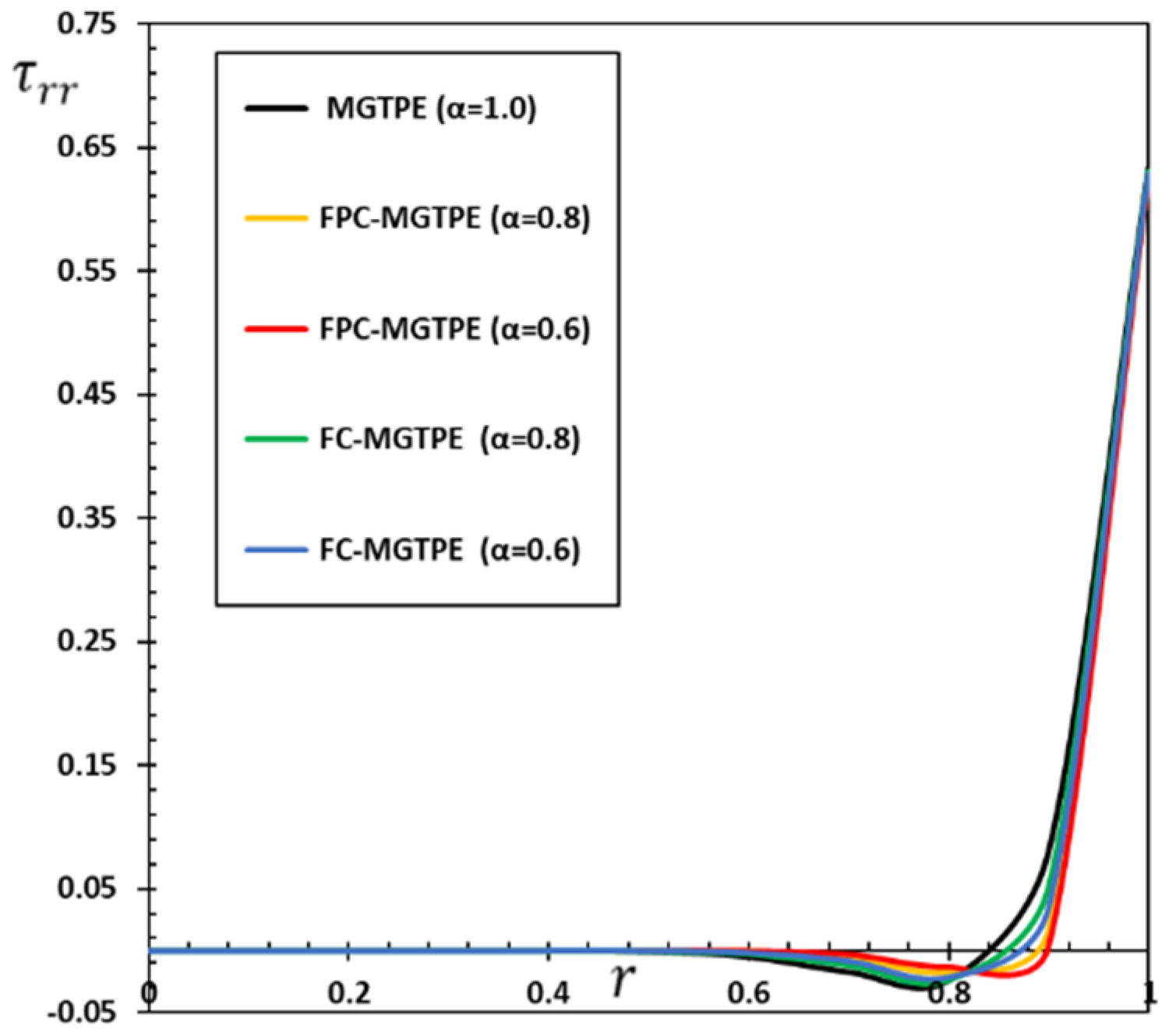
5.1. Comparative Analysis of Conventional and Proportional Caputo Derivative

Regarding integral and differential operators of variable orders, fractional calculus has been around for just as long as conceptional calculus, which works with non-negative integers. Researchers examined the possibility of modifications of classical calculus operators because not all real occurrences could be described using them. Fractional operators proved to be effective tools for simulating long-memory processes and various other processes found in the physical sciences, chemical engineering, electromagnetism, mechanical design, and other fields. An operator based on the proportional derivatives of a function relative to another function is introduced in this paper, which can be developed in tandem with the formulations in [14]. For the fractional operators, a new kernel that is built from an exponential function and depends on it was suggested.
This section compared the Moore–Gibson–Thompson fractional photothermal model (FPC-MGTPE) with a constant proportional Caputo type fractional derivative and the fractional photothermal model using the conventional Caputo operator (FC-MGTPE). If the initial condition is set to zero, the conventional fractional Caputo operator’s Laplace transform will be in the following form:
L [ D t ( α ) f ( t ) ] = s α L [ f ( t ) ] f ( 0 ) = s α F ( s ) .
Two cases of constant proportionality can be taken into account in which [59]
k 1 ( α , t ) = 1 α   and   k 0 ( α , t ) = α , k 1 ( α , t ) = 1 α 2   and   k 0 ( α , t ) = α 2
As the distance r increases, Figure 1, Figure 2, Figure 3, Figure 4 and Figure 5 show how the studied fields vary over time. In order to calculate the effects of the fractional-order coefficients, we used α = 0.8 and α = 0.6 in the numerical calculations and estimates. Moreover, to check and validate the numerical results, a comparison was made with the conventional case where α = 1 .
The results show that there is a need for operators and fractal derivatives that reduce the patterns of different physical fields in accordance with the physical qualitative and experimental results. It can also be seen that the decay rate is faster in the case of using modified fractional models than in the case of the classical model. This clearly occurs in the case of the study of viscous and non-viscous materials. The figures show that when the fractional order factor decreases, the maximum amplitude of the studied physical fields also decreases.
Figure 1 displays the changes in the temperature increase in the opposite direction of the radius increase, and it can be seen that all the heat graphs start at the surface r = 1 , with their largest value, which represents the thermal shock on the surface of the sphere boundary, and then gradually decrease again until it vanishes. As illustrated in Figure 1, fractional derivatives have only a minor impact on the temperature distribution; in some cases, they are completely absent. Through the numerical results, we can take advantage of the advanced MGTPE fractal model, through which we are able to classify some materials according to the properties of the fractal order they possess. As a direct result of this, the fractal parameter represented by the symbol α becomes an increasingly important way to measure how well a substance transfers heat. At the terminus of the sphere’s radius, the FC-MGTPE and FPC-MGTPE model graphs converge to a point where they have zero value. It shows that the thermal wave has moved at a limited rate in the FC-MGTPE and FPC-MGTPE theories but not in the traditional MGTPE theory.
Figure 2 illustrates how different types of fractional derivatives change the amount of deformation u in a radial direction. L’Hôpital’s rule was applied to reduce singularities in the domain center of the analyzed functions. The graph shows that the fractional differential greatly impacts how the deformation changes over time. In order to meet the regularity requirement, all displacement curves in the case of all the different models always converge and tend towards zero inside the sphere because there are no singular points. The numerical data and graphs illustrate that the displacement u starts with negative values, rapidly increases to a maximum of positive values, and then gradually decreases to zero. In addition, it can be demonstrated that, despite the disparities in values, the displacement diagrams of each model converge. Thus, it may be concluded that thermal parameters have little effect on displacement changes. The FC-MGTPE concept has a significantly greater displacement variation than the FPC-MGTPE theory, and the constant proportional Caputo fractional operator significantly affects displacement.
Radial and hoop stress are indicated in the radial direction in Figure 3 and Figure 4, respectively. Regarding fractional-order characteristics, the radial stress is obviously tensile, while the hoop stress is compressive. In the FPC-MGTPE concept, the thermomechanical wave action is smoother than it is in the FC-MGTPE version and in the normal scenario in which there is no fractional derivative, which is one of the most remarkable conclusions that can be derived from the evaluation of the various field patterns. It follows from these figures that the decrease in the order of the fractional derivative α leads to an increase in the amplitude of stresses. In order to be consistent with the boundary conditions, it is important to remember that the radial stress always begins at zero. After that, it gradually lowers until it approaches the lowest value at the sphere’s surface, progressively rising until it approaches zero again.
Figure 5 depicts the five curves for the carrier density N versus the radius r that were calculated using various fractional photo-thermoelasticity models. These curves are shown in relation to one another. As a result of charge carrier recombination, the carrier density N increases close to the surface of the sphere and then steadily declines as the radial distance increases until it achieves a steady state. Each of the five curves exhibits the same behavior but at different values, and they all have a peak point.
When it comes to a wide range of flexible photothermal formulations, Maxwell’s stress τ r r against r can be shown as shown in Figure 6. Because photothermal semiconductors behave physically, electromagnetic waves can only travel a certain distance before reaching their destination. We can also see that the curves behave consistently across models, with minor variations. The fractional-order parameter affects Maxwell’s stress. Because of this, the inclusion of a fractional-order parameter is critical in this model.
In order to make the theoretical framework of fractal thermoelasticity simpler, the links between current models are illustrated in this study. The current model may theoretically be reduced to a pre-existing fractional theory. When solving for the heat conduction equation, numerical findings reveal that the order of the Caputo derivative has an important impact on the sphere’s temperature history. There is less of an impact on the temporal history of temperature in the sphere when comparing the Riemann–Liouville and Caputo fractional heat transport models. When applied to control theory, this novel Caputo-style fractional operator is a modification of the conventional proportional derivative [14,15]. Control theory will benefit from the new fractional operator. In light of the physical significance of the beginning conditions, the Caputo fractional extension is the focus here.

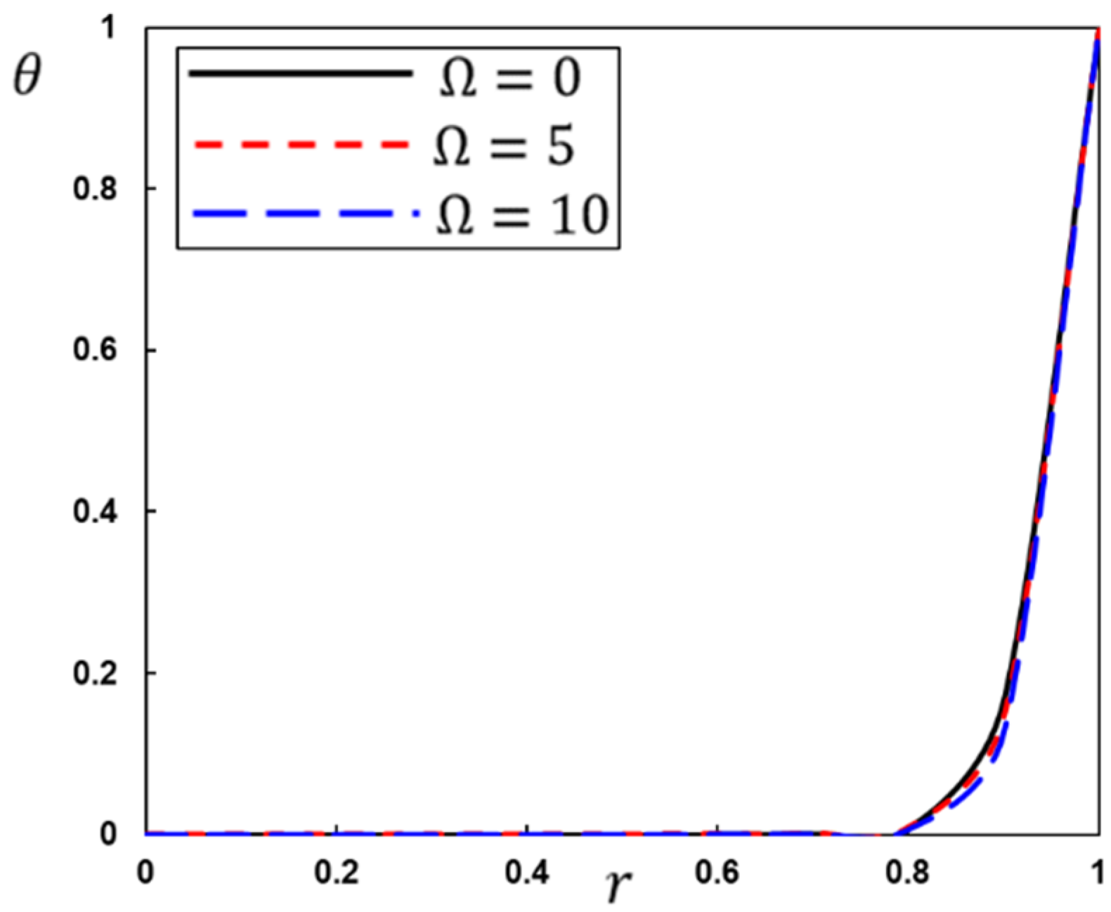
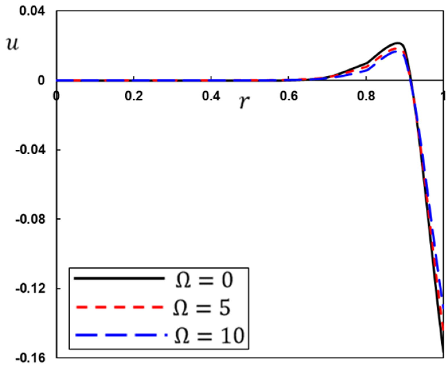
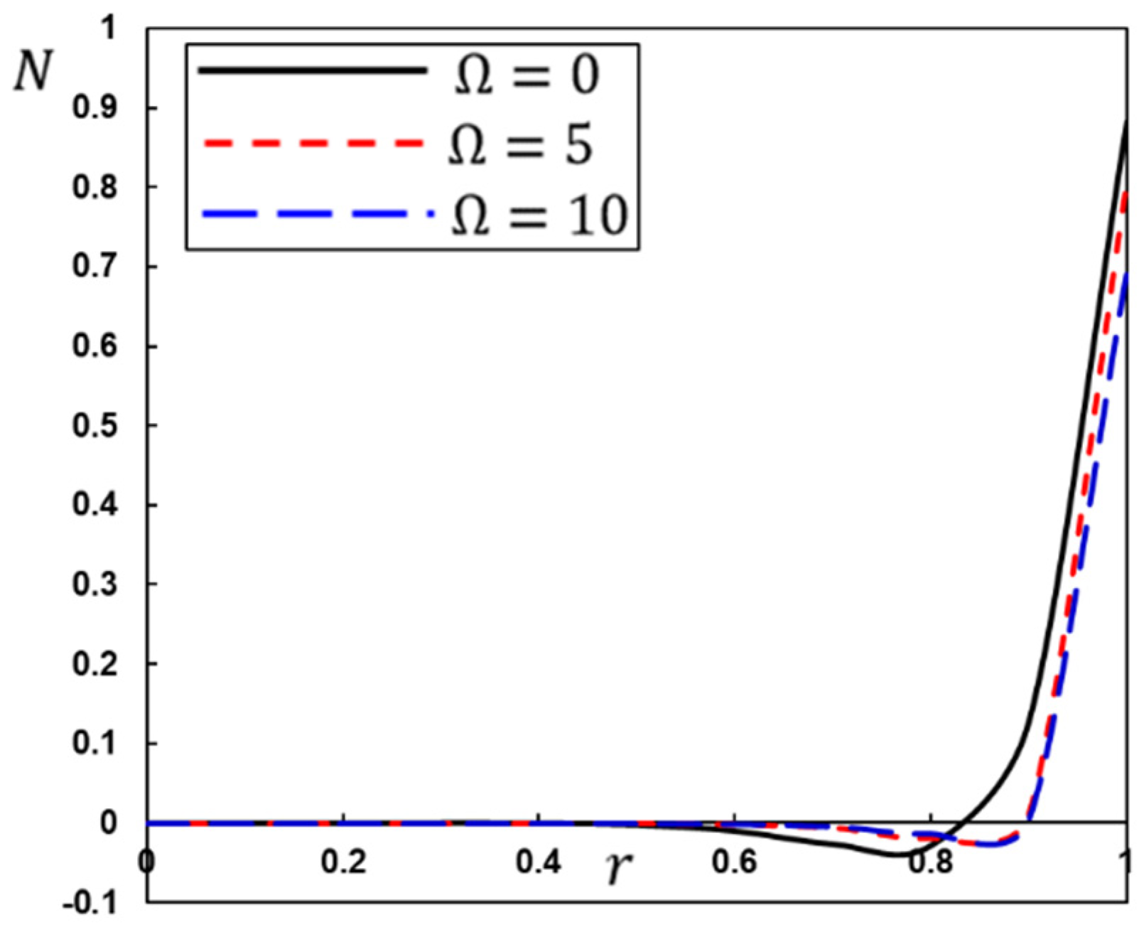
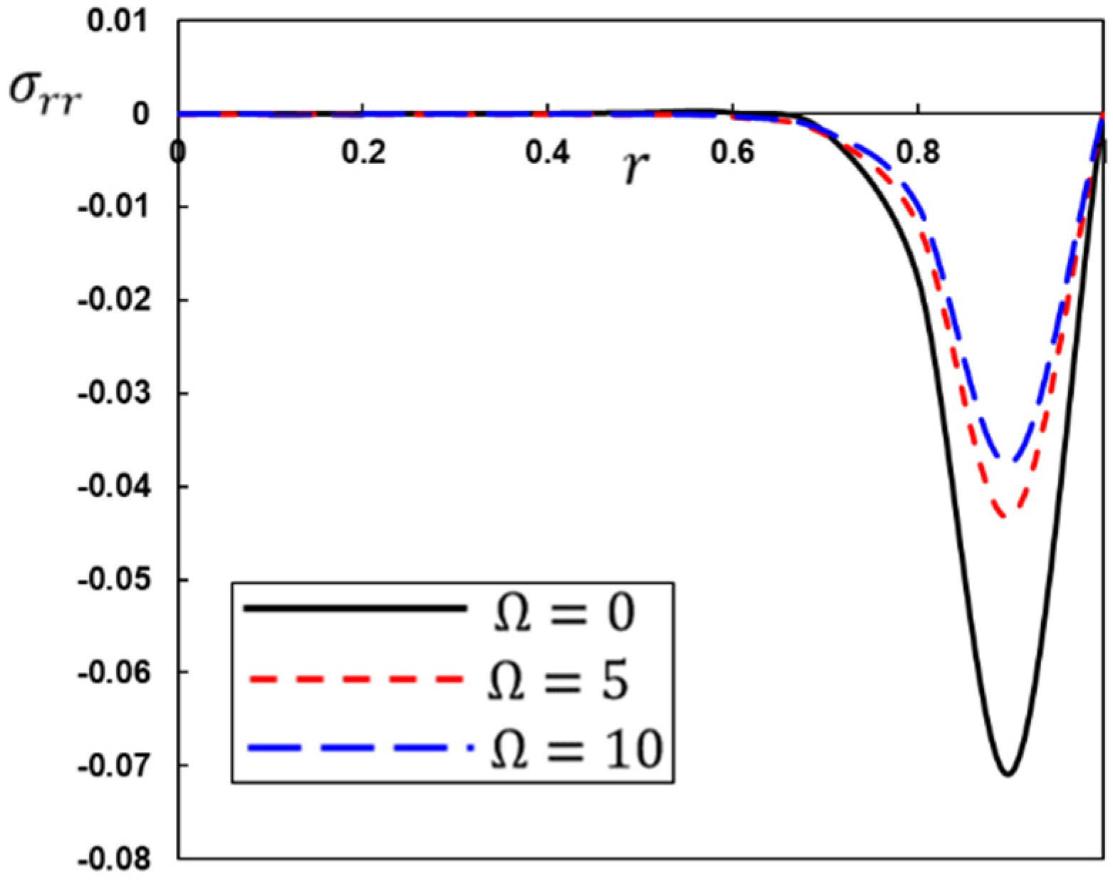
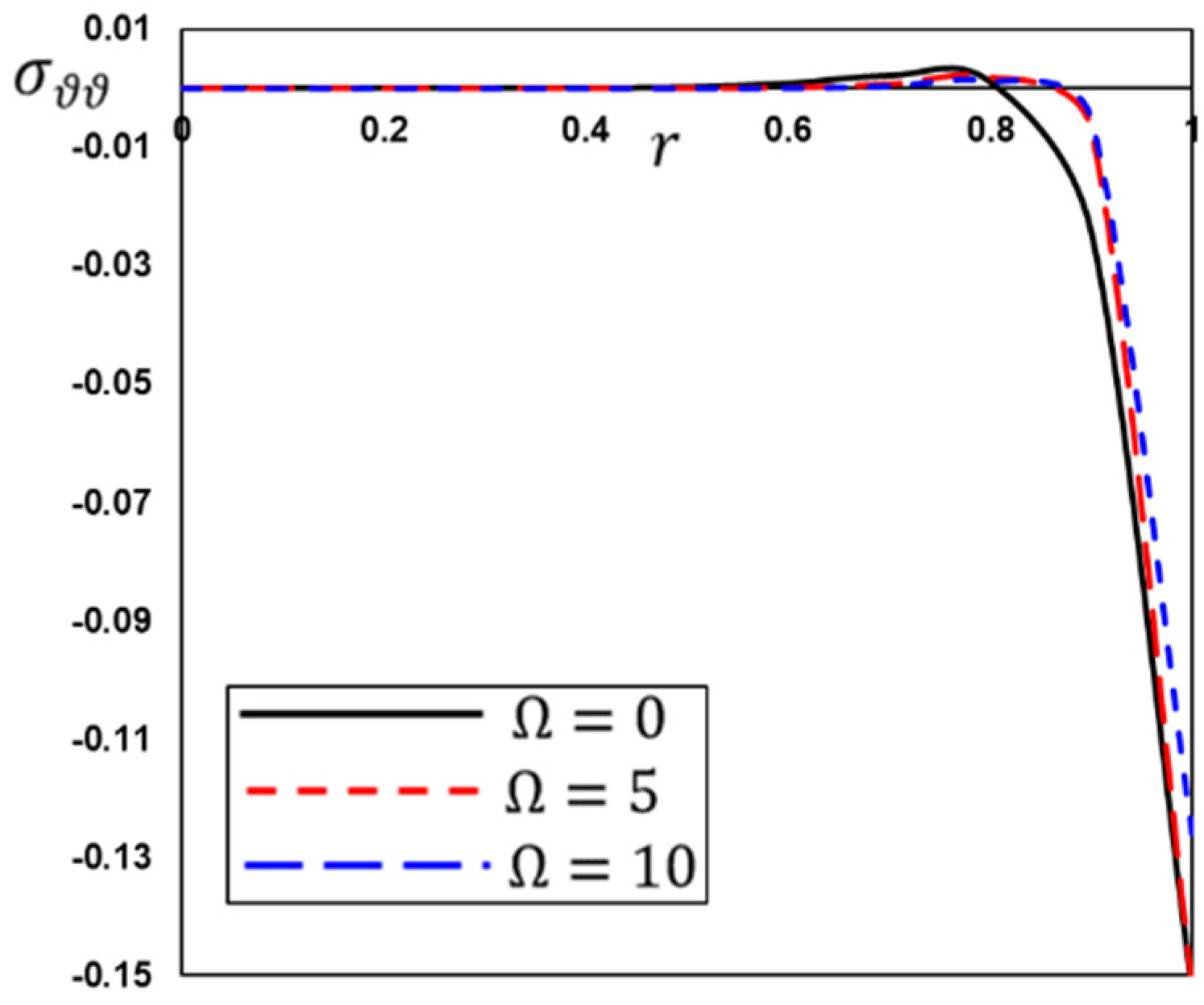
5.2. The Rotation Influence

Solid motion can be divided into translational and rotational movements, which play an essential role in heat and mass transfer in various engineering processes. Research into thermal light wave propagation in a spinning medium appears to be restricted, judging from a review of the available research on the topic. The Earth, the moon, and other planets all move at an angle, so it makes sense to explore how planar ductile heat waves or thermally induced magnetic waves propagate across rotating media where the temperature changes.
Various non-dimensional photothermal fields in generalized heat and mass transfer theory are examined in this section concerning the rotation parameter (MGTPT). Everything is better compared to what would have happened if there had been no rotation. When it comes to comparing the angular velocity, we used three numbers to express it: With Ω = 5 ,   10 , the revolving case is selected, whereas the nonrotating case is chosen with a value of Ω = 0 . Results for the relevant fields of analysis are shown in Figure 7, Figure 8, Figure 9, Figure 10, Figure 11 and Figure 12. A slight effect of rotation on temperature increment θ , radial displacement u , and Maxwell’s stress τ r r can be observed in Figure 7, Figure 8, and Figure 12. This is in line with what was found in the literature [60,61,62]. Increasing the rotation parameter Ω decreases all three field variables: θ , u , and τ r r , as can be seen in Figure 7, Figure 8, and Figure 12. For various rotation parameters Ω , the temperature curve is shown in Figure 7. The temperature drops radially from the sphere’s surface to its center, as depicted in the figure, whereas the temperature drops as the rotation parameter Ω increases. There is a gradual decrease in the amount of radial displacement as the rotational parameter Ω rises, as shown in Figure 8. According to the thermal stress σ r r profile, the rotational factor ( Ω ) has an enormous impact.
As can be seen in Figure 9, Figure 10 and Figure 11, the rotational parameter Ω greatly affects the carrier density N as well as the thermal stresses σ r r and σ ϑ ϑ . Figure 10 depicts the relationship between radius and rotational parameter Ω to demonstrate how thermal stresses change with increasing radius. With increasing rotation parameters, the radial stress σ r r decreases while the hoop stress σ ϑ ϑ rises, as seen in Figure 10 and Figure 11, respectively. Raising rotational factor Ω raises carrier density numerical data, as seen in Figure 10.

6. Conclusions

An expanded photothermal Moore–Gibson–Thompson heat conduction model with various fractional proportional integrals and derivatives is suggested in this work. The fractional variation impact of the new constant proportional Caputo type fractional derivative operator is more appropriate and adaptive than that of the Caputo derivative operator. It can be utilized to explain various real-world scenarios successfully. When using the Laplace transform method, a combination of fractional operators with a singular kernel is used to model the system of equations. It was found that angular velocity has two general patterns for different values of the fractional parameter for both small and large amounts of time, depending on the fractional parameter. Based on the proposed fractional photothermal model, a numerical study of the problem of one-dimensional thermoelasticity of a rotating spherical solid body was presented. The most important observations and conclusions obtained can be summarized as follows:
  • In contrast to other models, the model that was proposed allows heat-elastic light waves to move at a measurable speed. In addition, the model analyzes how heat, plasma, and elastic waves interact in semiconductor materials. The fractional proposed model makes it possible to derive, as special cases, several thermoelastic and photothermal models that have already been proposed;
  • Some materials can be further classified based on the Caputo-type constant relative partial derivative factor, which may be the basis for using temperature-dependent refractory materials in terms of photothermal conductivity;
  • The thermal relaxation time that was introduced in the new model had a prominent role in the behavior of the physical fields, as it was found that its presence reduces the propagation of mechanical and thermal optical waves within the medium. L’Hôpital’s rule was used to remove the singular points in the functions that were looked at in the middle of the sphere;
  • The rotation speed of the medium affects the behavior of many physical fields in addition to electro-optical mechanical waves;
  • In future work, the current work can be generalized by using the fractional derivative with time-dependent variable fractional orders. Moreover, the results obtained in this study can be generalized to other fields such as experimental physics, thermal efficiency, material design, and geophysics. Finally, these theoretical results will be very useful for scientists who are working on experimental results in the heat flow of a second-order viscoelastic fluid and a Maxwell fluid.

Author Contributions

Conceptualization, O.M. and A.E.A. Formal analysis, O.M. and A.E.A.; Investigation, M.A.; Methodology, A.E.A. and M.A.; Software, M.A.; Writing—original draft, M.A.; Writing—review & editing, O.M. and A.E.A. All authors have read and agreed to the published version of the manuscript.

Funding

The authors extend their appreciation to the Deputyship for Research& Innovation, Ministry of Education, Saudi Arabia for funding this research work through the project number (QU-IF-2-5-3-26923).

Institutional Review Board Statement

Not applicable.

Informed Consent Statement

Not applicable.

Data Availability Statement

Not applicable.

Acknowledgments

The authors extend their appreciation to the Deputyship for Research& Innovation, Ministry of Education, Saudi Arabia for funding this research work through the project number (QU-IF-2-5-3-26923). The authors also thank to Qassim University for technical support.

Conflicts of Interest

The authors declared no potential conflicts of interest with respect to the research, authorship, and publication of this article.

Notations and Symbols

λ ,   μ Lam e s   constants  
α t thermal   expansion  
C E specific heat
γ = ( 3 λ + 2 μ ) α t thermal   coupling  
T 0 reference   temperature  
θ = T T 0 temperature change
T absolute temperature
u i displacement   components  
e = u k , k cubical   dilatation
σ i j stress   tensor
e i j strain   tensor
δ i j Kronecker’s delta function
n 0 equilibrium carrier concentration
K i j thermal   conductivity   tensor
G carrier photogeneration
K thermal   conductivity
ρ material   density  
Ω angular   velocity  
C i j k l elastic   constants  
d n = ( 3 λ + 2 μ ) δ n diffusion   coupling  
N carrier   density
i , j , k 1 ,   2 ,   3
Q ource   of   heat
E g semiconducting   energy   gap
δ n electronic deformation
D E diffusion
q heat   flux  
κ thermal   activation   coupling  
τ ifetime   of   photogenerated   electron  
F external   forces

References

  1. Jarad, F.; Abdeljawad, T.; Rashid, S.; Hammouch, Z. More properties of the proportional fractional integrals and derivatives of a function with respect to another function. Adv. Differ. Equ. 2020, 2020, 303. [Google Scholar] [CrossRef]
  2. Kilbas, A.; Srivastava, H.M.; Trujillo, J.J. Theory and Application of Fractional Differential Equations; North-Holland Mathematics Studies; Elsevier: Amsterdam, The Netherlands, 2006; Volume 204. [Google Scholar]
  3. Magin, R.L. Fractional Calculus in Bioengineering; Begell House Publishers: Danbury, CT, USA, 2006. [Google Scholar]
  4. Podlubny, I. Fractional Differential Equations; Academic Press: San Diego, CA, USA, 1999. [Google Scholar]
  5. Jarad, F.; Alqudah, M.A.; Abdeljawad, T. On more general forms of proportional fractional operators. Open Math. 2020, 18, 167–176. [Google Scholar] [CrossRef]
  6. Al-Mdallal, Q.M. On fractional-Legendre spectral Galerkin method for fractional Sturm-Liouville problems. Chaos Solitons Fractals 2018, 116, 261–267. [Google Scholar] [CrossRef]
  7. Caputo, M.; Fabrizio, M. A new definition of fractional derivative without singular kernel. Prog. Fract. Differ. Appl. 2015, 1, 73–85. [Google Scholar]
  8. Atangana, A.; Baleanu, D. New fractional derivative with non-local and non-singular kernel. Therm. Sci. 2016, 20, 757. [Google Scholar] [CrossRef]
  9. Jarad, F.; Abdeljawad, T.; Hammouch, Z. On a class of ordinary differential equations in the frame of Atangana–Baleanu fractional derivative. Chaos Solitons Fractals 2018, 117, 16–20. [Google Scholar] [CrossRef]
  10. Yavuz, M.; Özdemir, N. Comparing the new fractional derivative operators involving exponential and Mittag-Leffler kernel. Discret. Contin. Dyn. Syst. 2020, 13, 995–1006. [Google Scholar] [CrossRef]
  11. Nazir, G.; Shah, K.; Alrabaiah, H.; Khalil, H.; Khan, R.A. Fractional dynamical analysis of measles spread model under vaccination corresponding to non-singular fractional order derivative. Adv. Differ. Equ. 2020, 2020, 171. [Google Scholar] [CrossRef]
  12. Katugampola, U.N. A new approach to generalized fractional derivatives. Bull. Math. Anal. Appl. 2014, 6, 1–15. [Google Scholar]
  13. Jarad, F.; Abdeljawad, T.; Alzabut, J. Generalized fractional derivatives generated by a class of local proportional derivatives. Eur. Phys. J. Spec. Top. 2017, 226, 3457–3471. [Google Scholar] [CrossRef]
  14. Baleanu, D.; Fernandez, A.; Akgul, A. On a fractional operator combining proportional and classical differintegrals. Mathematics 2020, 8, 360. [Google Scholar] [CrossRef]
  15. Akgul, A.; Baleanu, D. Analysis and applications of the proportional Caputo derivative. Adv. Differ. Equ. 2021, 2021, 136. [Google Scholar] [CrossRef]
  16. Shiri, B.; Baleanu, D. A General Fractional Pollution Model for Lakes. Commun. Appl. Math. Comput. 2022, 4, 1105–1130. [Google Scholar] [CrossRef]
  17. Rahman, G.; Nisar, K.S.; Abdeljawad, T. Certain Hadamard proportional fractional integral inequalities. Mathematics 2020, 8, 504. [Google Scholar] [CrossRef]
  18. Anderson, D.R.; Ulness, D.J. On a fractional operator combining proportional. Adv. Dyn. Sys. Appl. 2015, 10, 109–137. [Google Scholar]
  19. Shiri, B.; Kong, H.; Wu, G.-C.; Luo, C. Adaptive Learning Neural Network Method for Solving Time-Fractional Diffusion Equations. Neural Comput. 2022, 34, 971–990. [Google Scholar] [CrossRef] [PubMed]
  20. Abbas, M.; Ragusa, M. On the hybrid fractional differential equations with fractional proportional derivatives of a function with respect to a certain function. Symmetry 2021, 13, 264. [Google Scholar] [CrossRef]
  21. Khaminsou, B.; Sudsutad, W.; Kongson, J.; Nontasawatsri, S.; Vajrapatkul, A.; Thaiprayoon, C. Investigation of Caputo proportional fractional integro-differential equation with mixed nonlocal conditions with respect to another function. AIMS Math. 2022, 7, 9549–9576. [Google Scholar] [CrossRef]
  22. Ahmed, I.E.; Abouelregal, A.E.; Mostafa, D.M. Photo-carrier dynamics in a rotating semiconducting solid sphere under modification of the GN-III model without singularities. Arch. Appl. Mech. 2022, 92, 2351–2370. [Google Scholar] [CrossRef]
  23. Adams, M.J.; Kirkbright, G.F. Thermal diffusivity and thickness measurements for solid samples utilising the optoacoustic effect. Analyst 1977, 102, 678–682. [Google Scholar] [CrossRef]
  24. Vargas, H.; Miranda, M.L.C. Photoacoustic and Re1ated Phototherma1 Technique. Phys. Rep. 1988, 161, 43–101. [Google Scholar] [CrossRef]
  25. Ferreira, S.O.; Ying An, C.; Bandeira, I.N.; Miranda, L.C.M.; Vargas, H. Photoacoustic measurement of the thermal diffusivity ofPb1−xSnxTe alloys. Phys. Rev. B 1989, 39, 7967–7970. [Google Scholar] [CrossRef] [PubMed]
  26. Stearns, R.G.; Kino, G.S. Effect of electronic strain on photoacoustic generation in silicon. Appl. Phys. Lett. 1985, 47, 1048–1050. [Google Scholar] [CrossRef]
  27. Lotfy, K.; El-Bary, A.; Ismail, E.A.; Atef, H.M. Analytical solution of a rotating semiconductor elastic medium due to a refined heat conduction equation with hydrostatic initial stress. Alex. Eng. J. 2020, 59, 4947–4958. [Google Scholar] [CrossRef]
  28. Gordon, J.P.; Leite RC, C.; Moore, R.S.; Porto SP, S.; Whinnery, J.R. Long-transient effects in lasers with inserted liquid samples. Bull. Am. Phys. Soc. 1964, 119, 501. [Google Scholar] [CrossRef]
  29. Todorovic, D.M.; Nikolic, P.M.; Bojicic, A.I. Photoacoustic frequency transmission technique: Electronic deformation mechanism in semiconductors. J. Appl. Phys. 1999, 85, 7716. [Google Scholar] [CrossRef]
  30. Song, Y.Q.; Todorovic, D.M.; Cretin, B.; Vairac, P. Study on the generalized thermoelastic vibration of the optically excited semiconducting microcantilevers. Int. J. Solids Struct. 2010, 47, 1871. [Google Scholar] [CrossRef]
  31. Abouelregal, A.E. Magnetophotothermal interaction in a rotating solid cylinder of semiconductor silicone material with time dependent heat flow. Appl. Math. Mech. 2021, 42, 39–52. [Google Scholar] [CrossRef]
  32. Abouelregal, A.E.; Sedighi, H.M.; Shirazi, A.H. The effect of excess carrier on a semiconducting semi-infinite medium subject to a normal force by means of Green and Naghdi approach. Silicon 2022, 14, 4955–4967. [Google Scholar] [CrossRef]
  33. Abouelregal, A.E.; Akgöz, B.; Civalek, Ö. Nonlocal thermoelastic vibration of a solid medium subjected to a pulsed heat flux via Caputo–Fabrizio fractional derivative heat conduction. Appl. Phys. A 2022, 128, 660. [Google Scholar] [CrossRef]
  34. Zakaria, K.; Sirwah, M.A.; Abouelregal, A.E.; Ali, F.R. Photo-Thermoelastic model with time-fractional of higher order and phase lags for a semiconductor rotating materials. Silicon 2021, 13, 573–585. [Google Scholar] [CrossRef]
  35. Lord, H.W.; Shulman, Y. A generalized dynamical theory of thermoelasticity. J. Mech. Phys. Solids 1967, 15, 299–309. [Google Scholar] [CrossRef]
  36. Green, A.E.; Lindsay, K.A. Thermoelasticity. J. Elast. 1972, 2, 1–7. [Google Scholar] [CrossRef]
  37. Tzou, D.Y. Experimental support for the lagging behaviour in heat propagation. J. Thermophys. Heat Transf. 1995, 9, 686–693. [Google Scholar] [CrossRef]
  38. Tzou, D.Y. A unified approach for heat conduction from macro to microscale. J. Heat Transf. 1995, 117, 8–16. [Google Scholar] [CrossRef]
  39. Green, A.E.; Naghdi, P.M. A re-examination of the basic postulates of thermomechanics. Proc. R. Soc. A Math. Phys. Eng. Sci. 1991, 432, 171–194. [Google Scholar]
  40. Green, A.E.; Naghdi, P.M. On undamped heat waves in an elastic solid. J. Therm. Stresses 1992, 15, 253–264. [Google Scholar] [CrossRef]
  41. Green, A.E.; Naghdi, P.M. Thermoelasticity without energy dissipation. J. Elast. 1993, 31, 189–208. [Google Scholar] [CrossRef]
  42. Abouelregal, A.E. A novel generalized thermoelasticity with higher-order time-derivatives and three-phase lags. Multidiscip. Modeling Mater. Struct. 2019, 16, 689–711. [Google Scholar] [CrossRef]
  43. Abouelregal, A.E.; Alesemi, M. Vibrational analysis of viscous thin beams stressed by laser mechanical load using a heat transfer model with a fractional Atangana-Baleanu operator. Case Stud. Therm. Eng. 2022, 34, 102028. [Google Scholar] [CrossRef]
  44. Boulaaras, S.; Choucha, A.; Scapellato, A. General Decay of the Moore–Gibson–Thompson Equation with Viscoelastic Memory of Type II. J. Funct. Spaces 2022, 2022, 9015775. [Google Scholar] [CrossRef]
  45. Quintanilla, R. Moore-Gibson-Thompson thermoelasticity. Math. Mech. Solids 2019, 24, 4020–4031. [Google Scholar] [CrossRef]
  46. Quintanilla, R. Moore-Gibson-Thompson thermoelasticity with two temperatures. Appl. Eng. Sci. 2020, 1, 100006. [Google Scholar] [CrossRef]
  47. Abouelregal, A.E. A comparative study of a thermoelastic problem for an infinite rigid cylinder with thermal properties using a new heat conduction model including fractional operators without non-singular kernels. Arch. Appl. Mech. 2022. [Google Scholar] [CrossRef] [PubMed]
  48. Aboueregal, A.E.; Sedighi, H.M.; Shirazi, A.H.; Malikan, M.; Eremeyev, V.A. Computational analysis of an infinite magneto-thermoelastic solid periodically dispersed with varying heat flow based on non-local Moore–Gibson–Thompson approach. Contin. Mech. Thermodyn. 2022, 34, 1067–1085. [Google Scholar] [CrossRef]
  49. Abouelregal, A.E.; Ersoy, H.; Civalek, Ö. Solution of Moore–Gibson–Thompson equation of an unbounded medium with a cylindrical hole. Mathematics 2021, 9, 1536. [Google Scholar] [CrossRef]
  50. Tibault, J.; Bergeron, S.; Bonin, H.W. On fnite-diference solutions of the heat equation in spherical coordinates. Numer. Heat Transf. Part A Appl. 1987, 12, 457–474. [Google Scholar]
  51. Xie, P.; He, T. Investigation on the electromagnetothermoelastic coupling behaviors of a rotating hollow cylinder with memory-dependent derivative. Mech. Based Des. Struct. Mach. 2021, 49, 1–19. [Google Scholar] [CrossRef]
  52. Song, Y.Q.; Bai, J.T.; Ren, Z.Y. Study on the reflection of photothermal waves in a semiconducting medium under generalized thermoelastic theory. Acta Mech. 2012, 223, 1545–1557. [Google Scholar] [CrossRef]
  53. Todorovic, D.M. Plasma, thermal, and elastic waves in semiconductors. Rev. Sci. Instrum. 2003, 74, 582. [Google Scholar] [CrossRef]
  54. Abouelregal, A.E. Fractional derivative Moore-Gibson-Thompson heat equation without singular kernel for a thermoelastic medium with a cylindrical hole and variable properties. ZAMM Z. Angew. Math. Und Mech. 2022, 102, e202000327. [Google Scholar] [CrossRef]
  55. Oliveira, E.C.; Machado, J.A.T. A Review of Definitions for Fractional Derivatives and Integral. Math. Probl. Eng. 2014, 2014, 238459. [Google Scholar] [CrossRef]
  56. Gao, F.; Chi, C. Improvement on conformable fractional derivative and its applications in fractional differential equations. J. Funct. Spaces 2020, 2020, 5852414. [Google Scholar] [CrossRef]
  57. Youssef, H.M.; El-Bary, A.A. Characterization of the photothermal interaction of a semiconducting solid sphere due to the mechanical damage and rotation under Green-Naghdi theories. Mech. Adv. Mater. Struct. 2022, 29, 889–904. [Google Scholar] [CrossRef]
  58. Honig, G.; Hirdes, U. A method for the numerical inversion of Laplace transform. J. Comp. Appl. Math. 1984, 10, 113–132. [Google Scholar] [CrossRef] [Green Version]
  59. Suleyman, C.; Ali, D. Equation including local fractional derivative and Neumann boundary conditions. Kocaeli J. Sci. Eng. 2020, 3, 59–63. [Google Scholar]
  60. Abouelregal, A.E.; Fahmy, M.A. Generalized Moore-Gibson-Thompson thermoelastic fractional derivative model without singular kernels for an infinite orthotropic thermoelastic body with temperature-dependent properties. ZAMM J. Appl. Math. Mech. Z. Angew. Math. Und Mech. 2022, 102, e202100533. [Google Scholar] [CrossRef]
  61. Abouelregal, A.E.; Mondal, S. Thermoelastic vibrations in initially stressed rotating microbeams caused by laser irradiation. Z. Angew. Math. Und Mech. 2022, 102, e202000371. [Google Scholar] [CrossRef]
  62. Nasr, M.E.; Abouelregal, A.E. Light absorption process in a semiconductor infinite body with a cylindrical cavity via a novel photo-thermoelastic MGT model. Arch. Appl. Mech. 2022, 92, 1529–1549. [Google Scholar] [CrossRef]
Figure 1. The temperature variation θ for different fractional derivatives.
Mathematics 10 03087 g001
Figure 2. The displacement variation u for different fractional derivatives.
Mathematics 10 03087 g002
Figure 3. The radial stress variation σ r r for different fractional derivatives.
Mathematics 10 03087 g003
Figure 4. The hoop stress variation σ ϑ ϑ for different fractional derivatives.
Mathematics 10 03087 g004
Figure 5. The carrier density N for different fractional derivatives.
Mathematics 10 03087 g005
Figure 6. Maxwell’s stress τ r r for different fractional derivatives.
Mathematics 10 03087 g006
Figure 7. The temperature variation θ for different rotation parameter Ω .
Mathematics 10 03087 g007
Figure 8. The displacement variation u for different rotation parameter Ω .
Mathematics 10 03087 g008
Figure 9. The carrier density N for different rotation parameter Ω .
Mathematics 10 03087 g009
Figure 10. The radial stress variation σ r r for different rotation parameter Ω .
Mathematics 10 03087 g010
Figure 11. The hoop stress variation σ ϑ ϑ for different rotation parameter Ω .
Mathematics 10 03087 g011
Figure 12. Maxwell’s stress τ r r for different rotation parameter Ω .
Mathematics 10 03087 g012
Publisher’s Note: MDPI stays neutral with regard to jurisdictional claims in published maps and institutional affiliations.

