A Robust Variable Selection Method for Sparse Online Regression via the Elastic Net Penalty

Abstract

Variable selection has been a hot topic, with various popular methods including lasso, SCAD, and elastic net. These penalized regression algorithms remain sensitive to noisy data. Furthermore, “concept drift” fundamentally distinguishes streaming data learning from batch learning. This article presents a method for noise-resistant regularization and variable selection in noisy data streams with multicollinearity, dubbed canal-adaptive elastic net, which is similar to elastic net and encourages grouping effects. In comparison to lasso, the canal adaptive elastic net is especially advantageous when the number of predictions (p) is significantly larger than the number of observations (n), and the data are multi-collinear. Numerous simulation experiments have confirmed that canal-adaptive elastic net has higher prediction accuracy than lasso, ridge regression, and elastic net in data with multicollinearity and noise.

1. Introduction

Most traditional algorithms are built on closed-world assumptions and use fixed training and test sets, which makes it difficult to cope with changeable scenarios, including the streaming data issue. However, most data in practical applications are provided as data streams. One of their common characteristics is that the data will continue to grow over time, and the uncertainty introduced by the new data will influence the original model. As a result, learning from streaming data has become more essential [1,2,3] in machine learning and data mining communities. In this article, we employ the online gradient descent (OGD) framework proposed by Zinkevich [4]. It is a real-time, streaming online technique that updates the model on top of the trained model once per piece of data, making the model time-sensitive. In this article, we will provide a novel noise-resistant variable selection approach for handling noisy data streams with multicollinearity.

Since the 1960s, the variable selection issue has been much research literature. Since Hirotugu Akaike [5] introduced the AIC criterion, variable selection techniques have advanced, including more classic methods such as subset selection and coefficient shrinkage [6]. Variable selection methods based on penalty functions were developed to optimize computational efficiency and accuracy. Using a multivariate linear model as an illustration, e.g.,

$$y={\beta }_0+x_1{\beta }_1+...+x_p{\beta }_p+ϵ,$$

where the parameter vector is $\beta ={[{\beta }_0,{\beta }_1,...,{\beta }_p]}^T$, the parameters are estimated by methods such as OLS and Maximum Likelihood. The penalty function that balances the complexity of the model is added to this to construct a new penalty objective function. This penalty objective function is then optimized (maximized or minimized) to obtain parameter estimates. Its general framework is:

$$R\left(\beta \right)+P_{\lambda }\left(\right|\beta \left|\right),$$

where $R\left(\beta \right)$ is loss function and $P_{\lambda }\left(\right|\beta \left|\right)$ is a penalty function. This strategy enables the S/E (selection/Estimation) phase of the subset selection method to be done concurrently by compressing part of the coefficients to zero, significantly lowering computing time and minimizing the chance of the subset selection method becoming unstable. The most often employed of these are bridge regression [7], ridge regression [8], and lasso [9], with bridge regression having the following penalty function:

$$P_{\lambda }\left(\left|\beta \right|\right)=\lambda \sum _{j=1}^p{\left|{\beta }_j\right|}^m,\lambda ,m>0,$$

where $\lambda$ is an adjustment parameter, since the ridge regression model introduces the ${\ell }_2$-norm, it has a more stable regression effect and outperforms OLS in prediction. While the lasso method is an ordered, continuous process, it offers the advantages of low computing effort, quick calculation, parameter estimation continuity, and adaptability to high-dimensional data. However, lasso has several inherent disadvantages, one being the absence of the Oracle characteristic [10]. The adaptive lasso approach was proposed by Zou [11]. Similar to ADS (adaptive Dantzig selector) [12] for DS (Datnzig selector) [13] the adaptive lasso is an improvement on the lasso method with the same level of coefficient compression. The adaptive lasso has Oracle properties [11]. According to Zou [11], the greater the least squares estimate of a variable, the more probable it is to be a variable in the genuine model. Hence, the penalty for it should be reduced. The adaptive lasso method’s penalty function is specified as:

$$P_{\lambda }\left(\left|\beta \right|\right)=\lambda \sum _{j=1}^p\frac{1}{{\left|\widehat{{\beta }_j}\right|}^{\theta }}\left|{\beta }_j\right|,\lambda ,\theta >0,$$

where $\lambda$ and $\theta$ are adjustment parameters.

With several sets of explanatory variables known to be strongly correlated, the lasso method is powerless if the researcher wants to keep or remove a certain group of variables. Therefore, Yuan and Lin [14] proposed the group lasso method in 2006. The basic idea is to assume that there are J groups of strongly correlated variables, namely $G_1,\cdots ,G_J$, and the number of variables in each group is $p_1,\cdots ,p_J$, and ${\beta }_{G_j}={\left({\beta }_j\right)}^{j\in G_j}$ as the corresponding element of the sub-variables. The penalty function for the group Lasso method:

$$P_{\lambda }\left(\left|\beta \right|\right)=\lambda \sum _{j=1}^J\left|\right|{\beta }_{G_j}{\left|\right|}_{K_j},$$

where ${∥{\beta }_{G_j}∥}_{K_j}={\left({\beta }_{G_j}^T{K}_j{\beta }_{G_j}\right)}^{1/2}$ is the elliptic norm determined by the positive definite matrix $K_j$.

Chesneau and Hebiri [15] proposed the grouped variables lasso method and investigated its theory in 2008. They proved this bound is better in some situations than the one achieved by the lasso and the Dantzig selector. The group variable lasso exploits the sparsity of the model more effectively. Percival [16] developed the overlapping groups lasso approach, demonstrating that permitting overlap does not remove many of the theoretical features and benefits of lasso and group lasso. This method can encode various structures as collections of groups, extending the group lasso method. Li, Nan, and Zhu [17] proposed the MSGLasso (Multivariate Sparse Group Lasso) method. The method can effectively remove unimportant groups and unimportant individual coefficients within important groups, especially for the $p\gg n$ problem. It can flexibly handle a variety of complex group structures, such as overlapping, nested, or multi-level hierarchies.

The prediction accuracy of the lasso drastically reduces when confronted with multi-collinear data. A novel regularisation approach dubbed elastic net [18] has been presented to address these issues. Elastic net estimation may be conceived as a combination of lasso [9] and ridge regression [8] estimation. Compared to lasso, the elastic net approach performs better with data of the kind $p\gg n$ with several co-linearities between variables. However, a basic elastic net is incapable of handling noisy data. To address the difficulties above, we propose canal-adaptive elastic net method in this article. This technique offers four significant advantages:

• This model is efficient at handling streaming data. The suggested canal-adaptive elastic net dynamically updates the regression coefficients $\beta$ for regularised linear models in real-time. Each time a batch of data is fetched, the OGD framework enables updating the original model. Can handle stream data more effectively.
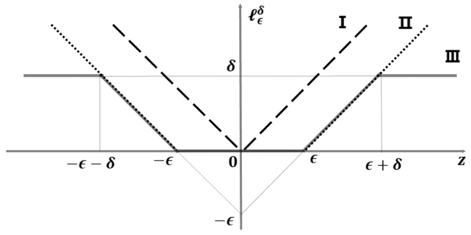
• The model has a sparse representation. As illustrated in Figure 1, only a tiny subsection of samples with residuals in the ranges $\left(-ϵ-\delta ,-ϵ\right)$ and $\left(ϵ,ϵ+\delta \right)$ are used to adjust the regression parameters. As a result, the model has perfect scalability and decreases computing costs.
• The improved loss function confers on the model a significant level of noise resistance. By dynamically modifying the $\delta$ parameter, noisy data with absolute errors (bigger than the threshold parameter $\delta +ϵ$) are recognized and excluded from being employed to alter the regression coefficients.
• The ${\ell }_1$-norm and ${\ell }_2$-norm are employed. Can handle the scenario of $p\gg n$ in the data more effectively. Simultaneous automatic variable selection and continuous shrinkage and can select groups of related variables. Overcoming the effects of data multicollinearity.

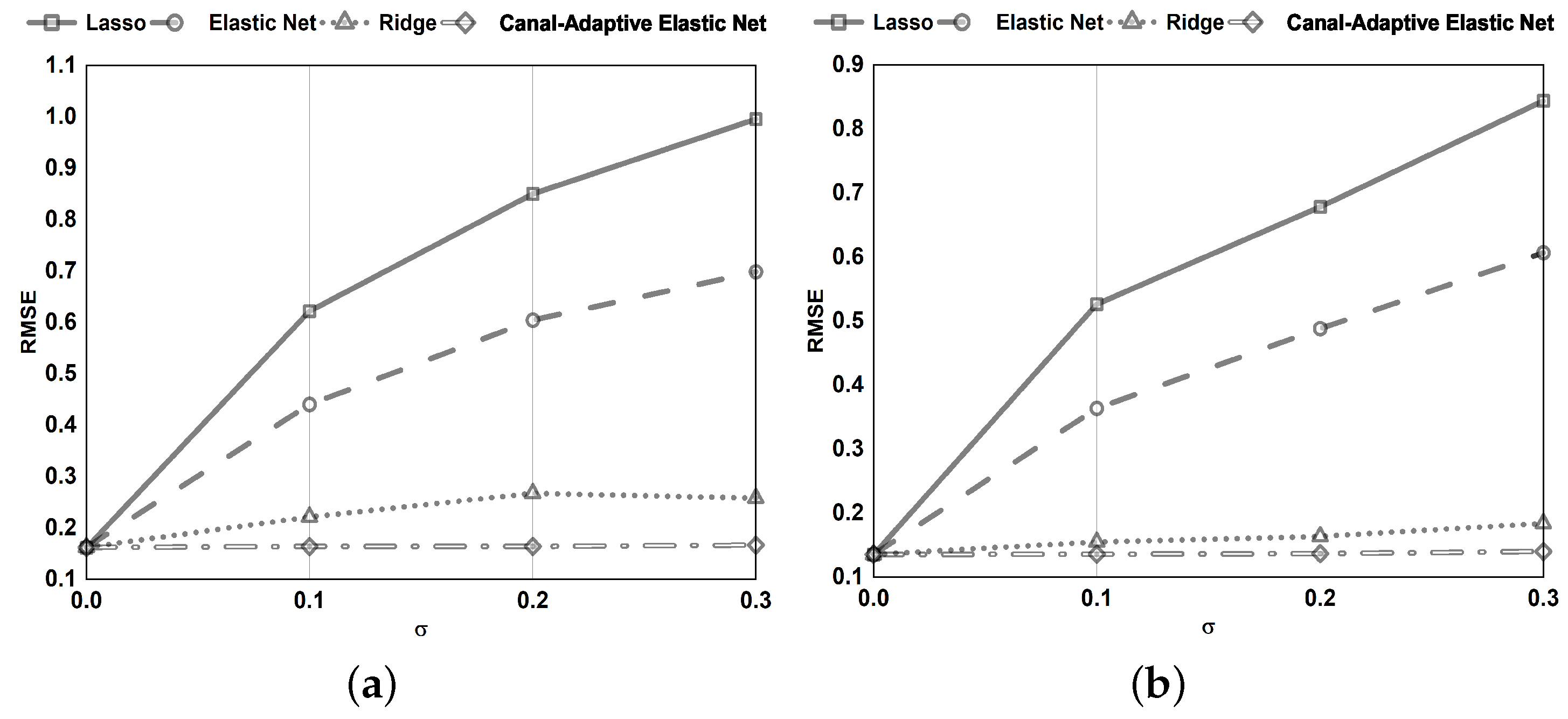
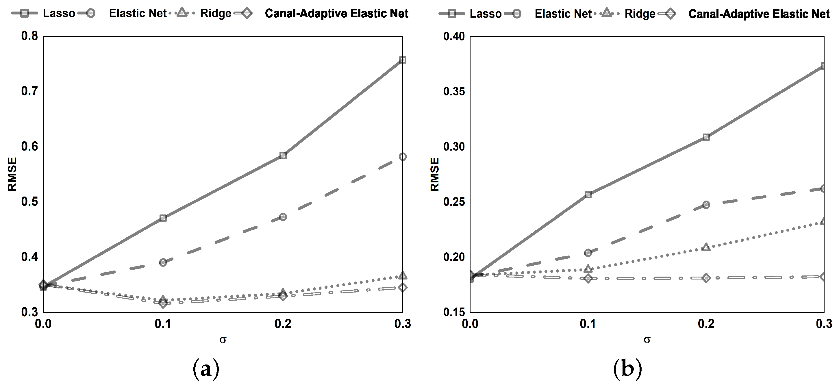
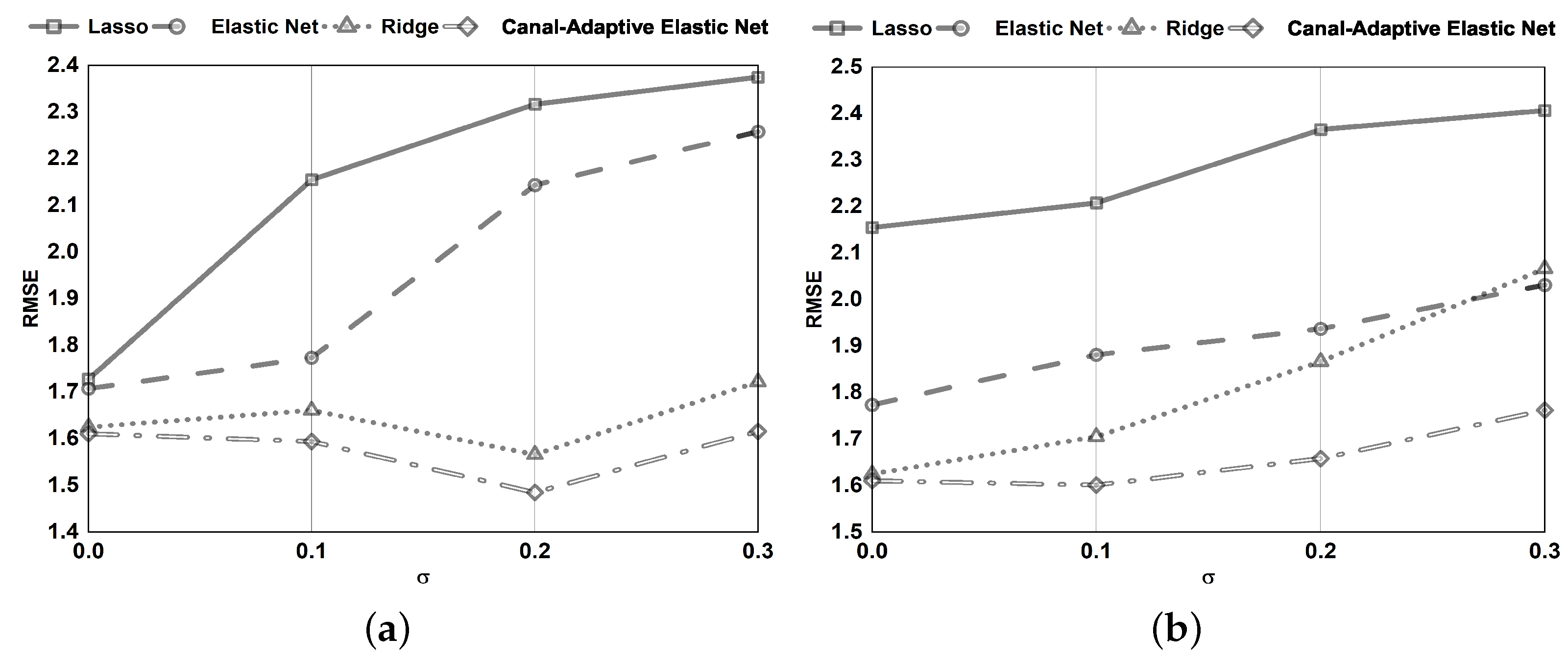
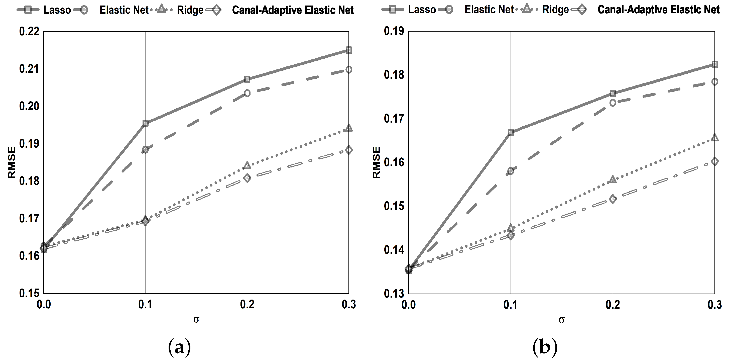
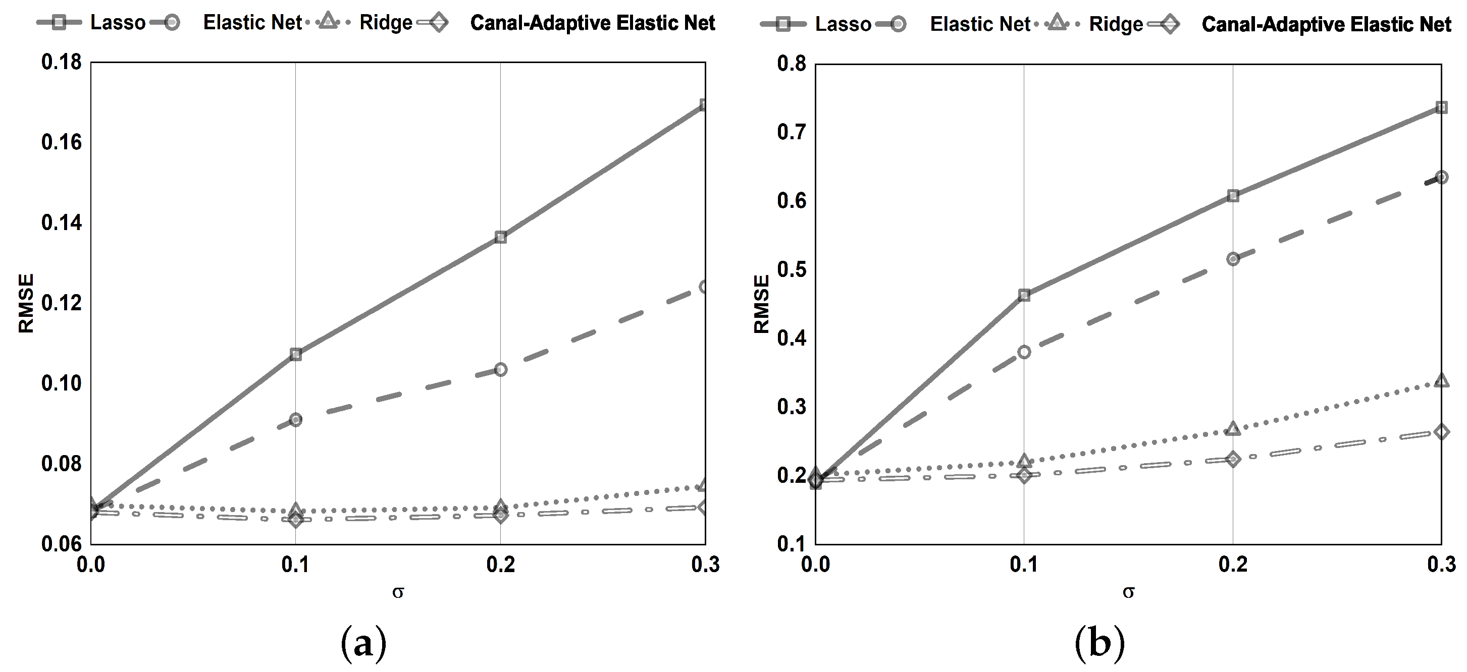
The rest of this paper is structured in the following manner. Section 2 reviews some studies on variable selection, noise-tolerant loss functions, data multicollinearity, and streaming data. Section 3 summarizes previous work on the penalty aim function and then introduces the linear regression noise-resistant online learning technique. In Section 4, we conduct numerical simulations and tests on benchmark datasets to compare the canal-adaptive elastic net presented in this research to lasso, ridge regression, and elastic net. Finally, Section 5 presents a concise discussion to conclude the paper.

2. Related Works

Variable selection has always been an important issue in building regression models. It has been one of the hot topics in statistical research since it was proposed in the 1960s, generating much literature on variable selection methods. For example, the Japanese scholar Akaike [5] proposed the AIC criterion based on the maximum likelihood method, which can be used both for the selection of independent variables and for setting the order of autoregressive models in time series analysis. Schwarz [19] proposed the BIC criterion based on the Bayes method. Compared to AIC, BIC strengthens the penalty and thus is more cautious in selecting variables into the model. All the above methods achieve variable selection through a two-step S/E (Selection/Estimation) process, i.e., first selecting a subset of variables in an existing sample according to a criterion. A subset of variables is selected from the existing sample according to a criterion (Selection). Then the unknown coefficients are estimated from the sample (Estimation). Because the correct variable is unknown in advance, the S-step is biased, which increases the risk of the E-step. To overcome this drawback, Seymour Geisser [20] proposed Cross-validation. Later on, variable selection methods based on penalty functions emerged. Tibshirani [9] proposed LASSO (Least Absolute Shrinkage and Selection Operator) inspired by the NG (Nonnegative Garrote) method. The lasso method avoids the drawback of over-reliance on the original least squares estimation of the NG method. As Fan and Li [21] pointed out that lasso does not possess the Oracle property, they thus proposed a new variable selection method, the SCAD (Smoothly Clipped Absolute Deviation) method, and proved that it has the Oracle property. Zou [11] proposed the adaptive lasso method based on the lasso. The variable selection methods with structured penalties (e.g., features are dependent and/or there are group structures between features) have become more popular because of the ever-increasing need to handle complex data, such as elastic net and group lasso [14].

While investigating noise-resistant loss functions, we generated interest in the truncated loss function. The losses generate learning models that are robust to substantial quantities of noise. Xu et al. [22] demonstrated that truncation could tolerate much higher noise for enjoying consistency than without truncation. The robust variable selection is a novel concept that incorporates robust losses from the robust statistics area into the model. Formed models that perform well empirically in noisy situations [23,24,25].

The concept of multicollinearity refers to the linear relationships between the independent variables in multiple regression analysis. Multicollinearity occurs when the regression model incorporates variables that are highly connected not only with the dependent variable but also to each other [26]. Some research has explored and discussed the challenges associated with multicollinearity in regression models, emphasizing that the primary issue of multicollinearity is uneven and biased standard errors and unworkable interpretations for the results [27,28]. There are many strategies for handling multicollinearity, one of which is ridge regression [29,30].

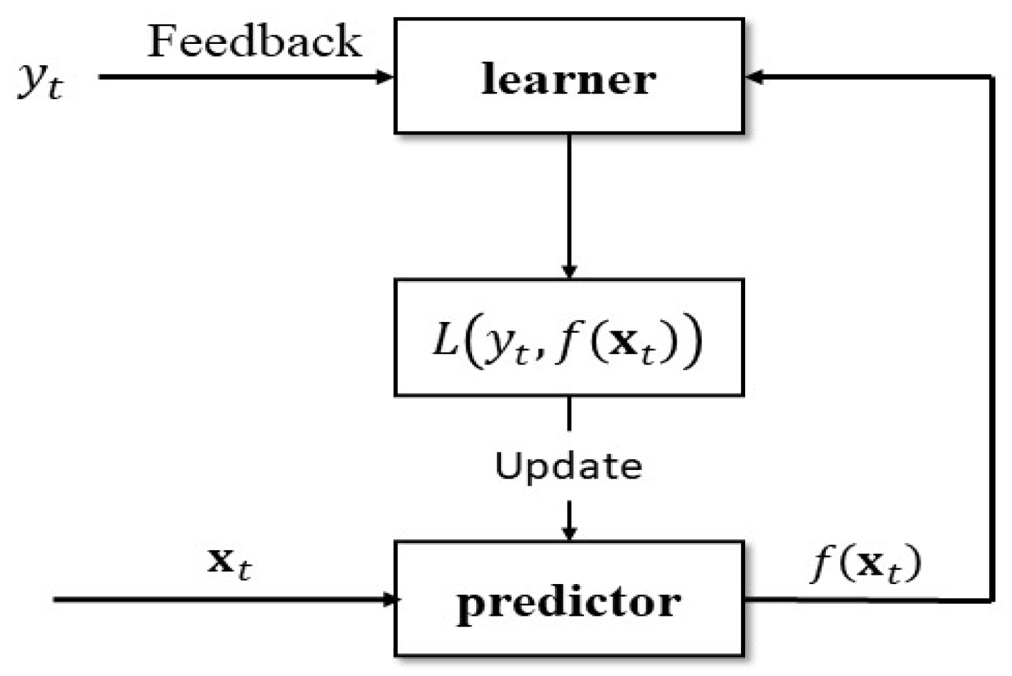
Many studies have been conducted over the last few decades on inductive learning approaches such as lasso [9], artificial neural networks [31,32]. Support vector regression [33], among others. These methods have been applied successfully to a variety of real-world problems. However, their usual implementation causes the simultaneous availability of all training data [34], making them unsuitable for large-scale data mining applications and streaming data mining tasks [35,36]. Compared to the traditional batch learning framework, the online learning algorithm (shown in Figure 2) is another framework for learning samples in a streaming fashion, which has the advantage of scalability and real-time. In recent years, great attention has been paid to developing online learning methods in the machine learning community, such as online ridge regression [37,38], adaptive regularization for lasso [39], projection [40] and bounded online gradient descent algorithm [41].

3. Method

Most currently available online regression algorithms learn information from clean data. Because of flaws in the human labeling process and sensor failures, noisy data are unavoidable and damaging. In this section, we propose a noise-tolerant online learning algorithm for the linear regression of streaming data. We employed a noise-resilient loss function, dubbed canal loss, for regression based on the well-known $ϵ-insensitive$ loss, inspired by the ramp loss designed for classification problems. In addition, we will use a novel method to adjust the $ϵ$ and $\delta$ dynamics of the canal loss parameters.

3.1. Canal-Adaptive Elastic Net

For a given n-group of data ${\left\{\left({\mathbf{x}}_i,y_i\right)\right\}}_{i=1}^n,y_i\in \mathbb{R}$, we consider a simple liner regression model:

$$\mathbf{y}=\mathbf{X}\beta +ϵ,$$

where $\mathbf{y}={\left(y_1,y_2,\cdots ,y_n\right)}^T$ is the response and $\mathbf{X}=\left({\mathbf{x}}_1,{\mathbf{x}}_2,\cdots ,{\mathbf{x}}_p\right)$ is the models column full rank design matrix, ${\mathbf{x}}_j={\left(x_{1j},x_{2j},\cdots ,x_{nj}\right)}^T,j=1,2,\cdots ,p$ is the n-dimensional explanatory variable, $\beta ={\left({\beta }_1,{\beta }_2,\cdots ,{\beta }_p\right)}^T$ is the associated vector of regression coefficient, $ϵ$ are i.i.d random errors vector with mean of 0. Without losing generality we can assume that the response is centered and the predictors are standardized after a location and scale transformation,

$$\sum _{i=1}^n{y}_i=0,\sum _{i=1}^n{x}_{ij}=0,\sum _{i=1}^n{x}_{ij}^2=1,j=1,2,\dots ,p.$$

However, if $\mathbf{X}$ is not column full rank, or if the linear correlation between some columns is significant, the determinant of ${\mathbf{X}}^{\mathbf{T}}\mathbf{X}$ is close to 0, i.e., ${\mathbf{X}}^{\mathbf{T}}\mathbf{X}$ is close to singular. The traditional OLS method lacks stability and reliability. To solve the above problem, Hoerl and Kennard [20] proposed ridge regression:

$$RidgeRegression:L\left(\beta \right)=\sum _{i=1}^n{\left(y_i-{\mathbf{x}}_i\beta \right)}^2+\lambda \sum _{j=1}^p{\beta }_j^2.$$

The penalty technique improves OLS by transforming the unfit problem into a fit problem. It loses the unbiasedness of OLS in exchange for higher numerical stability and obtains higher computational accuracy. Although ridge regression can effectively overcome the high correlation between variables and improve the prediction accuracy, model selection cannot be made with ridge regression alone. Therefore, Tibshirani [9] proposed the primary lasso criterion:

$$Lasso:L\left(\beta \right)=\sum _{i=1}^n{\left(y_i-{\mathbf{x}}_i\beta \right)}^2+\lambda \sum _{j=1}^p\left|{\beta }_i\right|,$$

where $\lambda >0$ is a fixed adjustment parameter. Lasso is a penalized ordinary least squares method. Based on the singularity of the derivative of the penalty function at zero, the coefficients of the insignificant variables are compressed to zero, and a lighter compression is given to the significant independent variables with larger estimates. The accuracy of the parameter estimates is ensured.

However, lasso also has some inherent drawbacks: lasso does not have the Oracle property. It has the disadvantage of selecting at most n variables when considering data of sample size $(p>n)$. Where numerous characteristics are interrelated, lasso selects one of these characteristics. Lasso is less effective than ridge regression when handing independent variables with multicollinearity. Therefore, Zou and Hastie proposed the elastic net:

$$ElasticNet:L({\lambda }_1,{\lambda }_2,\beta )=\sum _{i=1}^n{\left(y_i-{\mathbf{x}}_i\beta \right)}^2+{\lambda }_2\sum _{j=1}^p{\beta }_j^2+{\lambda }_1\sum _{j=1}^p\left|{\beta }_j\right|.$$

The elastic net uses both ${\ell }_1$-norm and ${\ell }_2$-norm as linear regression models with a priori canonical terms. It combines the advantages of lasso and ridge regression. It is a method to solve the group variable selection with unknown variable grouping. Compared with the lasso, elastic net also improves handling data with sample size $(p>n)$ and data with multicollinearity among variables. Unfortunately, because of the loss function’s shortcomings, the elastic net cannot erase the effects caused by noisy data.

To obtain a noise-resilient elastic net-type estimator. Based on the classical $ϵ-insensitive$ loss function $l_{ϵ}\left(z\right)$=$max\left\{0,\left|z\right|-ϵ\right\}$. Canal loss with noise-resilient parameter $\delta$ is proposed:

$$l_{ϵ}^{\delta }\left(z_i\right)=min\left\{\delta ,max\left\{0,\left|z_i\right|-ϵ\right\}\right\}$$

where $z_i=y_i-{\mathbf{x}}_i\beta$, $ϵ>0$ and $\delta >0$ are the threshold tuning parameter. The canal loss function’s upper bound is maintained as a constant, i.e., $\delta$, which considerably reduces the negative influence of outliers and makes it a noise-resistant loss function. Using the advantages of canal loss, we modify the elastic net and propose the canal-adaptive elastic net as a new method. We define the canal-adaptive elastic net as:

$$Canal-AdaptiveElasticNet:L({\lambda }_1,{\lambda }_2,\beta )=\sum _{i=1}^n{l}_{ϵ}^{\delta }\left(z_i\right)+{\lambda }_2\sum _{j=1}^p{\beta }_j^2+{\lambda }_1\sum _{j=1}^p{\widehat{w}}_j\left|{\beta }_j\right|,$$

where ${\lambda }_1$, ${\lambda }_2>0$, ${\widehat{\mathbf{w}}}_{\mathbf{j}}={\left|{\widehat{\beta }}_j\left(en\right)\right|}^{-\gamma }$ for $j=1,\cdots ,p$, $\gamma$ is a positive constant. We can also define ${\widehat{w}}_j=\infty$ when ${\widehat{\beta }}_j\left(en\right)=0$. ${\widehat{\beta }}_j\left(en\right)$ is the weight to correct the regression coefficient ${\beta }_j$. We define $\widehat{\mathbf{\beta }}\left(\mathit{en}\right)$ as:

$$\widehat{\beta }\left(en\right)=\underset{\mathbf{\beta }}{argmin}\sum _{i=1}^n{l}_{ϵ}^{\delta }\left(z_i\right),$$

where $\widehat{\mathbf{\beta }}\left(\mathit{en}\right)={\left({\widehat{\beta }}_1\left(en\right),{\widehat{\beta }}_2\left(en\right),\cdots ,{\widehat{\beta }}_p\left(en\right)\right)}^T$.

The canal loss approximates the absolute loss in the process of $ϵ\to 0$ and $\delta \to +\infty$, which is more clearly expressed as:

$$\underset{ϵ\to 0,\delta \to +\infty }{lim}{\ell }_{ϵ}^{\delta }\left(z_i\right)=\underset{ϵ\to 0,\delta \to +\infty }{lim}min\left\{\delta ,max\left\{0,\left|z_i\right|-ϵ\right\}\right\}=\left|z_i\right|.$$

The proposed canal-adaptive elastic net is predicted to be robust to outliers and to have the property of sparse representation.

3.2. Online Learning Algorithm for Canal-Adaptive Elastic Net

We employed the online gradient descent algorithm (OGD) and presented the minimization optimization strategy to solve the canal-adaptive elastic net model efficiently

$$L({\lambda }_1,{\lambda }_2,\beta )=\sum _{t=1}^n{l}_{ϵ}^{\delta }\left(z_t\right)+{\lambda }_2\sum _{j=1}^p{\beta }_j^2+{\lambda }_1\sum _{j=1}^p{\widehat{w}}_j\left|{\beta }_j\right|,$$

(1)

where $z_t=y_t-{\mathbf{x}}_t\beta$.

First, the literature has proposed numerous methods for estimating the regularisation parameter, including cross-validation, AIC, and BIC. We minimize the BIC-type objective function to optimize the regularisation parameter, which makes the calculation quicker and ensures consistency in variable selection, i.e.,

$$\underset{\lambda }{min}\sum _{t=1}^n{l}_{ϵ}^{\delta }\left(z_t\right)+{\lambda }_2\sum _{j=1}^p{\beta }_j^2+{\lambda }_1\sum _{j=1}^p{\widehat{w}}_j\left|{\beta }_j\right|-log({\lambda }_1+{\lambda }_2)log\left(n\right).$$

Second, although Equation (1) is not a convex optimization problem, it can be restated as a difference in convex (DC) programming issue. This problem may be solved using the Concave-Convex Procedure (CCCP). However, because CCCP is a batch learning algorithm, it does not meet real-time processing requirements when handling streaming data. We used the well-known OGD framework in our work to arrive at a near-optimal solution. This is a compromise between accuracy and scalability. To minimize Equation (1) by OGD, we reformulate it as:

$$\underset{\beta }{argminL\left(\beta \right)}\iff \underset{\beta }{argmin}\sum _{t=1}^n\underset{J_t\left(\beta \right)}{\underbrace{\left[l_{ϵ}^{\delta }\left(z_t\right)+{\lambda }_2\sum _{j=1}^p{\beta }_j^2+{\lambda }_1\sum _{j=1}^p{\widehat{w}}_j\left|{\beta }_j\right|\right]}},$$

and then, based on the basic structure of the OGD algorithm, we solve this optimization problem,

$${\beta }^{\left(t\right)}={\beta }^{(t-1)}-{\eta }_t{\nabla }_{\beta }{J}_t\left(\beta \right)\left|{}_{\beta ={\beta }^{(}t-1).}\right.$$

(2)

Here, ${\eta }_t$ is the t-th step that satisfies the following constraints ${\sum }_{t=1}^n{\eta }_t^2<\infty$ and ${\sum }_{t=1}^n{\eta }_t=\infty$. when $n\to \infty$ [42]. Unlike the exact computation of the full gradient of $L({\lambda }_1,{\lambda }_2,\beta )$, the notation ${{\nabla }_{\beta }{J}_t\left(\beta \right)|}_{\beta ={\beta }^{(}t-1)}$ denotes the derivative of $J_t\left(\beta \right)$ with respect to $\beta ={\beta }^{(t-1)}$ of the derivative. We can deduce ${{\nabla }_{\beta }{J}_t\left(\beta \right)|}_{\beta =\beta (t-1)}$ as following:

$${{\nabla }_{\beta }{J}_t\left(\beta \right)|}_{\beta =\beta (t-1)}=\left\{\begin{array}{c}-{\mathbf{x}}_t+2{\lambda }_2{\beta }^{(t-1)}+{\lambda }_1(-{\gamma \left|{\beta }^{(t-1)}\right|}^{-\gamma -1}sign\left({\beta }^{(t-1)}\right)\left|{\beta }^{(t-1)}\right|+{\left|{\beta }^{(t-1)}\right|}^{-\gamma }sign\left({\beta }^{(t-1)}\right)),\hfill \\ \mathrm{if}-ϵ-\delta <z_t<-ϵ,\hfill \\ {\mathbf{x}}_t+2{\lambda }_2{\beta }^{(t-1)}+{\lambda }_1(-{\gamma \left|{\beta }^{(t-1)}\right|}^{-\gamma -1}sign\left({\beta }^{(t-1)}\right)\left|{\beta }^{(t-1)}\right|+{\left|{\beta }^{(t-1)}\right|}^{-\gamma }sign\left({\beta }^{(t-1)}\right)),\hfill \\ \mathrm{if}ϵ<z_t<ϵ+\delta ,\hfill \\ 2{\lambda }_2{\beta }^{(t-1)}+{\lambda }_1(-{\gamma \left|{\beta }^{(t-1)}\right|}^{-\gamma -1}sign\left({\beta }^{(t-1)}\right)\left|{\beta }^{(t-1)}\right|+{\left|{\beta }^{(t-1)}\right|}^{-\gamma }sign\left({\beta }^{(t-1)}\right)),\hfill \\ \mathrm{otherwise},\hfill \end{array}\right.$$

(3)

where $z_t=y_t-{\mathbf{x}}_t{\beta }^{(t-1)}$, substituting the gradient Equation (3) into Equation (2),

$${\beta }^{\left(t\right)}=\left\{\begin{array}{c}{\beta }^{(t-1)}-{\eta }_t(-{\mathbf{x}}_{t}sign\left(z_t\right)+2{\lambda }_2{\beta }^{(t-1)}+{\lambda }_1(-{\gamma \left|{\beta }^{(t-1)}\right|}^{-\gamma -1}sign\left({\beta }^{(t-1)}\right)\left|{\beta }^{(t-1)}\right|+{\left|{\beta }^{(t-1)}\right|}^{-\gamma }sign\left({\beta }^{(t-1)}\right))),\hfill \\ \mathrm{if}ϵ<\left|z_t\right|<ϵ+\delta ,\hfill & \\ {\beta }^{(t-1)}-{\eta }_t(2{\lambda }_2{\beta }^{(t-1)}+{\lambda }_1(-{\gamma \left|{\beta }^{(t-1)}\right|}^{-\gamma -1}sign\left({\beta }^{(t-1)}\right)\left|{\beta }^{(t-1)}\right|+{\left|{\beta }^{(t-1)}\right|}^{-\gamma }sign\left({\beta }^{(t-1)}\right))),\hfill \\ \mathrm{otherwise}.\hfill \end{array}\right.$$

(4)

Finally, as shown in Equation (3), the proposed canal-adaptive elastic net contains a sparsity parameter $ϵ\ge 0$ and a noise-resilient parameter $\delta \ge 0$. The parameter $ϵ$ determines the sparsity of the proposed model, whereas $\delta$ indicates the level of noise elasticity. Proposing a strategy for adjusting the channel loss parameters is a pressing issue. $ϵ$ and $\delta$ are automatically iterated. In this study, we set the parameters:

$$\left\{\begin{array}{c}ϵ=\zeta \times mean\left\{\left|{\widehat{y}}_t\right|,\left|y_t\right|\right\},\hfill \\ \delta =\gamma \times mean\left\{\left|{\widehat{y}}_t\right|,\left|y_t\right|\right\}\hfill \end{array}\right.$$

(5)

Adjusting $ϵ$ and $\delta$ parameters is equivalent to adjusting $\zeta$ and $\gamma$. When $\gamma$ is set to 0, the algorithm does not learn any examples of ${\left\{({\mathbf{x}}_t,y_t)\right\}}_{t=1}^n$ and instead updates $\beta$ according to the regularization term. If $\gamma$ is sufficiently big, our canal-adaptive elastic net will withstand noisy data. The proposed canal-adaptive elastic net algorithm is summarized as Algorithm 1.

Algorithm 1 Noise-Resilient Online Canal-adaptive Elastic Net Algorithm.

Input: Initial ${\beta }^{\left(\mathbf{0}\right)}={\underset{d+1}{\underbrace{[1,1,\dots ,1]}}}^T$ estimate number of examples $\mathrm{n}$ and instance sequences

${\mathbf{x}}_t(t=1,\dots )$.

Output: Predict ${\widehat{y}}_t(t=1,\dots )$

1:${\mathbf{X}}_t={\left[1{\mathbf{x}}_t\right]}^T={\left[1,x_{1t},x_{2t},\dots ,x_{dt}\right]}^T$

2: for $t=1,\dots$ do

3:      Receive instance ${\mathbf{X}}_t$

4:      Predict value ${\widehat{y}}_t={\mathbf{X}}_t^T{\beta }^{(t-1)}$

5:      Receive true value $y_t$

6:      Update canal loss parameter $ϵ$ and $\delta$ according to Equation (5)

7:      Compute residual error $z_t={\widehat{y}}_t-y_t$

8:      if   $ϵ\le \left|z_t\right|<ϵ+\delta$

9:         Update ${\beta }^{\left(t\right)}={\beta }^{(t-1)}-{\eta }_t\left(-{\mathbf{x}}_{t}sign\left(z_t\right)+2{\lambda }_2{\beta }^{(t-1)}+{\lambda }_1\left(-\gamma {\left|{\beta }^{(t-1)}\right|}^{-\gamma -1}sign\left({\beta }^{(t-1)}\right)\left|{\beta }^{(t-1)}\right|+{\left|{\beta }^{(t-1)}\right|}^{-\gamma }sign\left({\beta }^{(t-1)}\right)\right)\right)$,

according to Equation (4).

10:      else

11:         Update ${\beta }^{\left(t\right)}={\beta }^{(t-1)}-{\eta }_t\left(2{\lambda }_2{\beta }^{(t-1)}+{\lambda }_1\left(-\gamma {\left|{\beta }^{(t-1)}\right|}^{-\gamma -1}sign\left({\beta }^{(t-1)}\right)\left|{\beta }^{(t-1)}\right|+{\left|{\beta }^{(t-1)}\right|}^{-\gamma }sign\left({\beta }^{(t-1)}\right)\right)\right)$,

according to Equation (4).

12:      end if

13: end for

4. Experiments

In this part, we perform experiments to evaluate the canal-adaptive elastic net algorithm performs. First, simulation studies on synthetic data with multicollinearity and noise are used to verify the method’s efficiency. Second, the model’s resistance to noise and the variable selection accuracy is evaluated using data sets with different noise proportions. Finally, we run thorough tests to assess the proposed algorithm’s performance on four benchmark prediction tasks. The benchmark datasets used in the experiments are available from the UCI Machine Learning repository and LIBSVMP website.

4.1. Simulation Settings

We evaluate the proposed noise-resilient online regression algorithm on synthetic data sets with noise and multicollinearity. We examine the proposed canal-adaptive elastic net method’s effectiveness in handling noisy and multi-collinear input and output data. In addition, we evaluated the canal-adaptive elastic net method’s performance in simulation trials with and without multicollinearity datasets. The simulation experiment is described in detail below.

4.1.1. The Case of Both Multicollinearity and Noise

This experiment indicates that canal-adaptive elastic net on streaming data outperforms lasso, ridge regression, and elastic net in handling multicollinearity data and is a suitable variable selection procedure for handling noisy data than the other three methods.

We simulate 200 observations in each example and set the feature dimension d as 10. We let ${\beta }_j=0.85$ for all j. The correlation coefficients between $x_i$ and $x_j$ were greater than 0.8 in their absolute values. We trained the model on 70% of the data and then tested it on 30% of the data. We conducted 20 randomized trials and determined the MAE, RMSE, the number of discards, discard rate, and average computation time of the model on the test data set using varied noise proportions for x and y.

We generated simulated the data from the true model,

$$y_t={\mathbf{x}}_t\beta +\rho {ϵ}_t,ϵ\sim N(0,1),$$

(6)

where $\rho =3$ and ${ϵ}_t$ is generated by the normal distribution $N\left(0,1\right)$. For a given t, the covariate ${\mathbf{x}}_t$ is constructed using a standard d-dimensional multivariate normal distribution, which assures that the components of ${\mathbf{x}}_t$ are independent and standard normal. Here, we change the noise ratio $\sigma$ from $\{0,0.1,0.2,0.3\}$. To be more precise, we randomly select some samples $\{{\mathbf{x}}_t,y_t\}$ with the ratio of $\sigma$, change the 6th explanatory variable of ${\mathbf{x}}_t$ to 0 in the training set, and then evaluate the learning model on real test datasets.

Table 1. Results of simulations of noisy explanatory variable x in the presence of data multicollinearity.

$\mathit{\sigma }$	Method	RMSE	MAE	Discarded Samples	Discarded Rate	Time (s)
0	Lasso	1.7274 ± 0.2074	9.6486 ± 2.2035	0	0.00%	0.0011
	Elastic Net	1.7739 ± 0.2324	9.8651 ± 3.6694	0	0.00%	0.0013
	Ridge Regression	1.6251 ± 0.2599	7.7511 ± 1.6699	0	0.00%	0.0012
	Canal-Adaptive Elastic Net	1.6109 ± 0.1826	7.0687 ± 1.8752	0	0.00%	0.0014
0.1	Lasso	2.1554 ± 0.3275	15.2898 ± 4.9195	0	0.00%	0.0011
	Elastic Net	1.7073 ± 0.2796	9.3282 ± 2.8530	0	0.00%	0.0013
	Ridge Regression	1.6610 ± 0.2693	8.2822 ± 2.5765	0	0.00%	0.0012
	Canal-Adaptive Elastic Net	1.5942 ± 0.2684	7.2797 ± 2.5177	26.000 ± 2.000	13.00%	0.0015
0.2	Lasso	2.3174 ± 0.2899	18.0449 ± 4.7368	0	0.00%	0.0012
	Elastic Net	2.1440 ± 0.3066	15.3115 ± 4.7714	0	0.00%	0.0013
	Ridge Regression	1.5664 ± 0.1476	7.7189 ± 1.4264	0	0.00%	0.0011
	Canal-Adaptive Elastic Net	1.4850 ± 0.1959	7.0048 ± 1.3591	44.000 ± 4.000	22.00%	0.0015
0.3	Lasso	2.3753 ± 0.3360	18.8495 ± 4.6064	0	0.00%	0.0012
	Elastic Net	2.2583 ± 0.2608	16.8451 ± 3.7473	0	0.00%	0.0013
	Ridge Regression	1.7206 ± 0.1009	9.0645 ± 1.7891	0	0.00%	0.0012
	Canal-Adaptive Elastic Net	1.6157 ± 0.1340	8.0100 ± 2.1617	72.000 ± 7.000	36.00%	0.0015

contains the results. Furthermore, to find out the effect of the noisy response variable y. We randomly altered the response variable y to 0 in the training set at a rate of $\sigma$ and then tested the learning model with the real test sample.

Table 2. Results of simulations of noise response variables y in the presence of data multicollinearity.

$\mathit{\sigma }$	Method	RMSE	MAE	Discarded Samples	Discarded Rate	Time (s)
0	Lasso	2.1554 ± 0.3275	15.2898 ± 4.9195	0	0.00%	0.0011
	Elastic Net	1.7739 ± 0.2324	9.8651 ± 3.6694	0	0.00%	0.0013
	Ridge Regression	1.6251 ± 0.2599	8.0043 ± 1.6699	0	0.00%	0.0012
	Canal-Adaptive Elastic Net	1.6109 ± 0.1826	7.6687 ± 1.8752	0	0.00%	0.0014
0.1	Lasso	2.2082 ± 0.3966	14.8886 ± 5.2407	0	0.00%	0.0012
	Elastic Net	1.8817 ± 0.2330	10.2875 ± 3.9768	0	0.00%	0.0015
	Ridge Regression	1.7057 ± 0.1853	9.0843 ± 2.6754	0	0.00%	0.0012
	Canal-Adaptive Elastic Net	1.6013 ± 0.1743	7.0020 ± 2.3720	76.000 ± 7.000	38.00%	0.0016
0.2	Lasso	2.3659 ± 0.3966	18.9535 ± 3.2407	0	0.00%	0.0012
	Elastic Net	1.9372 ± 0.2960	13.1065 ± 4.0957	0	0.00%	0.0013
	Ridge Regression	1.8668 ± 0.2369	9.8637 ± 2.8419	0	0.00%	0.0012
	Canal-Adaptive Elastic Net	1.6585 ± 0.2178	7.7834 ± 2.0399	84.000 ± 8.000	42.00%	0.0015
0.3	Lasso	2.4068 ± 0.2157	19.7197 ± 3.5115	0	0.00%	0.0011
	Elastic Net	2.0314 ± 0.2787	14.2434 ± 4.9863	0	0.00%	0.0014
	Ridge Regression	2.0668 ± 0.1779	14.4463 ± 1.6615	0	0.00%	0.0012
	Canal-Adaptive Elastic Net	1.7624 ± 0.3057	8.6620 ± 2.7414	90.000 ± 0.800	45.00%	0.0015

summarizes the corresponding findings. To make a comparison, the compared models are solved using the online gradient descent (OGD) method, i.e., lasso, ridge regression, elastic net, and canal-adaptive elastic net. In the simulated experiments, we set the two hyper-parameters $ϵ=0.1$ and $\delta =2.0$.

First, we show that the canal-adaptive elastic net can avoid interfering with the explanatory variable x. Analysis of RMSE and MAE indicates lasso deviates significantly from the true value. In contrast, canal-adaptive elastic net, ridge regression, performs admirably. Lasso is sensitive to multicollinearity in the data because of its nature. In the presence of noise, the proposed canal-adaptive elastic net method outperforms the other three competing methods. In particular, canal-adaptive elastic net significantly outperforms lasso, ridge regression, elastic net, and in the presence of high noise level $(\sigma =0.3)$. Because of the inherent drawbacks of the elastic net, its loss function can reduce the impact of noisy data to some extent. However, the negative impact of noisy data is still serious. Figure 3a illustrates the predictive performance of different algorithms. It can be observed that when data are multicollinearity and noisy, the canal-adaptive elastic net outperforms lasso, ridge regression, and elastic net. This shows that the canal-adaptive elastic net is a method capable of overcoming multicollinearity and is noise-resistant.

Each coefficient may have an influence when noisy data are present in the response variable y. In the presence of multicollinearity in the data, the proposed canal-adaptive elastic net significantly outperforms lasso, ridge regression, and elastic net. Due to the lasso itself, it does not predict data containing multicollinearity very well. The estimation of $\beta$ deviates far from the true coefficient $\beta$ than the other three methods. Compared with the lasso, ridge regression and elastic nets effectively overcome the effects of data with multicollinearity. However, their performance suffers when a certain level of noise is introduced. The prediction performance of the different models is provided in Figure 3b for a more detailed comparison of the models. Canal-adaptive elastic net outperforms the other three approaches in the presence of noisy data and data with multicollinearity. The results show that the canal-adaptive elastic net is a successful technique for overcoming multicollinearity and handling noisy data when the response variable y contains considerable noise.

4.1.2. The Case of Noise

In this subsection, we present simulation experiments comparing the performance of canal-adaptive elastic nets with three competing approaches (lasso, ridge regression, and elastic net) on a limited sample of streaming noise data (n = 5000, 10,000). This experiment explores the performance of the four methods for group variable selection with unknown variable grouping. Because of its nature, group lasso cannot be included in this experiment. In addition, we set the $\beta$ to $(1,-2,3,-4,5,-6,0,$$0,\dots ,0)$. Where the feature dimension d is 50, the first six regression coefficients are significant, whereas the following 44 are insignificant. The covariate ${\mathbf{x}}_t$ is created for a given t using a standard d-dimensional multivariate normal distribution, which ensures that the components of ${\mathbf{x}}_t$ are independent and standard normal. The response variables are generated according to Equation (6) where $\rho =0.5$ and ${ϵ}_t$ are generated from the normal distribution N (0,1).

Also, to investigate the effects of the noisy response variable y and the explanatory variable x, we applied a certain percentage of noise to the training dataset in the same way as in Section 4.1.1. We then tested the learning model with real test samples.

Table 3. Simulation results for noisy explanatory variable x.

n	$\mathit{\sigma }$	Method	RMSE	MAE	Discarded Samples	Discarded Rate	Time (s)
5000	0	Lasso	0.1618 ± 0.0018	0.8085 ± 0.0170	0	0.00%	0.1787
		Elastic Net	0.1627 ± 0.0014	0.8165 ± 0.0153	0	0.00%	0.3423
		Ridge Regression	0.1626 ± 0.0021	0.8154 ± 0.0229	0	0.00%	0.1951
		Canal-Adaptive Elastic Net	0.1621 ± 0.0031	0.8122 ± 0.0260	694 ± 32	13.89%	0.2663
	0.1	Lasso	0.1955 ± 0.0101	1.1882 ± 0.1182	0	0.00%	0.1702
		Elastic Net	0.1885 ± 0.0106	1.1054 ± 0.1214	0	0.00%	0.3072
		Ridge Regression	0.1697 ± 0.0047	0.8966 ± 0.0509	0	0.00%	0.186
		Canal-Adaptive Elastic Net	0.1693 ± 0.0059	0.8896 ± 0.0620	903 ± 25	18.07%	0.2528
	0.2	Lasso	0.2073 ± 0.0103	1.3278 ± 0.1382	0	0.00%	0.1706
		Elastic Net	0.2036 ± 0.0091	1.2797 ± 0.1239	0	0.00%	0.2939
		Ridge Regression	0.1841 ± 0.0063	1.0430 ± 0.0704	0	0.00%	0.1736
		Canal-Adaptive Elastic Net	0.1809 ± 0.0045	1.0084 ± 0.0548	1118 ± 18	22.37%	0.2442
	0.3	Lasso	0.2151 ± 0.0109	1.4320 ± 0.1292	0	0.00%	0.1685
		Elastic Net	0.2099 ± 0.0046	1.3597 ± 0.0636	0	0.00%	0.3036
		Ridge Regression	0.1941 ± 0.0107	1.1614 ± 0.1392	0	0.00%	0.1655
		Canal-Adaptive Elastic Net	0.1884 ± 0.0061	1.0968 ± 0.0707	1325 ± 29	26.52%	0.2329
10,000	0	Lasso	0.1354 ± 0.0010	0.8009 ± 0.0159	0	0.00%	0.466
		Elastic Net	0.1355 ± 0.0011	0.8010 ± 0.0127	0	0.00%	0.7631
		Ridge Regression	0.1358 ± 0.0017	0.8044 ± 0.0159	0	0.00%	0.7302
		Canal-Adaptive Elastic Net	0.1358 ± 0.0011	0.8054 ± 0.0138	1353 ± 50	13.54%	0.6464
	0.1	Lasso	0.1669 ± 0.0110	1.2193 ± 0.1625	0	0.00%	0.4322
		Elastic Net	0.1581 ± 0.0106	1.0950 ± 0.1466	0	0.00%	0.819
		Ridge Regression	0.1449 ± 0.0033	0.9172 ± 0.0476	0	0.00%	0.4735
		Canal-Adaptive Elastic Net	0.1434 ± 0.0035	0.8981 ± 0.0466	1889 ± 44	18.90%	0.6209
	0.2	Lasso	0.1758 ± 0.0048	1.3500 ± 0.0746	0	0.00%	0.4313
		Elastic Net	0.1737 ± 0.0075	1.3187 ± 0.1231	0	0.00%	0.778
		Ridge Regression	0.1560 ± 0.0087	1.0660 ± 0.1086	0	0.00%	0.4408
		Canal-Adaptive Elastic Net	0.1517 ± 0.0069	1.0067 ± 0.0921	2300 ± 34	23.00%	0.587
	0.3	Lasso	0.1825 ± 0.0060	1.4521 ± 0.0948	0	0.00%	0.5801
		Elastic Net	0.1785 ± 0.0053	1.3895 ± 0.0854	0	0.00%	0.7243
		Ridge Regression	0.1656 ± 0.0064	1.1980 ± 0.0919	0	0.00%	0.4343
		Canal-Adaptive Elastic Net	0.1603 ± 0.0045	1.1198 ± 0.0599	2661 ± 51	26.61%	0.5867

and

Table 4. Simulation results for noisy response variable y.

n	$\mathit{\sigma }$	Method	RMSE	MAE	Discarded Samples	Discarded Rate	Time (s)
5000	0	Lasso	0.1618 ± 0.0018	0.8085 ± 0.0170	0	0.00%	0.1787
		Elastic Net	0.1627 ± 0.0014	0.8165 ± 0.0153	0	0.00%	0.3423
		Ridge Regression	0.1626 ± 0.0021	0.8154 ± 0.0229	0	0.00%	0.1951
		Canal-Adaptive Elastic Net	0.1621 ± 0.0031	0.8122 ± 0.0260	694 ± 32	13.89%	0.2663
	0.1	Lasso	0.6225 ± 0.0767	12.3388 ± 3.0485	0	0.00%	0.1875
		Elastic Net	0.4406 ± 0.0607	6.7411 ± 1.8332	0	0.00%	0.3103
		Ridge Regression	0.2215 ± 0.0532	1.5738 ± 0.7018	0	0.00%	0.1983
		Canal-Adaptive Elastic Net	0.1641 ± 0.0031	0.8260 ± 0.0350	1126 ± 21	22.54%	0.2627
	0.2	Lasso	0.8503 ± 0.0511	23.1978 ± 2.9234	0	0.00%	0.1789
		Elastic Net	0.6047 ± 0.0648	13.0583 ± 3.1128	0	0.00%	0.3212
		Ridge Regression	0.2678 ± 0.0511	2.2870 ± 0.8511	0	0.00%	0.1956
		Canal-Adaptive Elastic Net	0.1643 ± 0.0040	0.8354 ± 0.0382	1539 ± 25	30.79%	0.2648
	0.3	Lasso	0.9959 ± 0.0761	31.8982 ± 5.2155	0	0.00%	0.1769
		Elastic Net	0.6990 ± 0.0836	17.7096 ± 4.2660	0	0.00%	0.2947
		Ridge Regression	0.2583 ± 0.0447	2.1066 ± 0.7001	0	0.00%	0.2001
		Canal-Adaptive Elastic Net	0.1668 ± 0.0030	0.8548 ± 0.0363	1973 ± 29	39.47%	0.2608
10,000	0	Lasso	0.1354 ± 0.0010	0.8009 ± 0.0159	0	0.00%	0.466
		Elastic Net	0.1355 ± 0.0011	0.8010 ± 0.0127	0	0.00%	0.7631
		Ridge Regression	0.1358 ± 0.0017	0.8044 ± 0.0159	0	0.00%	0.7302
		Canal-Adaptive Elastic Net	0.1358 ± 0.0011	0.8054 ± 0.0138	1353 ± 50	13.54%	0.6464
	0.1	Lasso	0.5265 ± 0.0631	12.4175 ± 2.8731	0	0.00%	0.4823
		Elastic Net	0.3636 ± 0.0573	6.3646 ± 2.0023	0	0.00%	0.7922
		Ridge Regression	0.1549 ± 0.0172	1.0593 ± 0.2253	0	0.00%	0.5049
		Canal-Adaptive Elastic Net	0.1360 ± 0.0019	0.8052 ± 0.0173	2274 ± 29	22.74%	0.641
	0.2	Lasso	0.6783 ± 0.0658	20.8429 ± 4.3086	0	0.00%	0.4626
		Elastic Net	0.4885 ± 0.0612	11.9550 ± 3.0504	0	0.00%	0.7855
		Ridge Regression	0.1638 ± 0.0224	1.1977 ± 0.3214	0	0.00%	0.4963
		Canal-Adaptive Elastic Net	0.1370 ± 0.0017	0.8204 ± 0.0242	3093 ± 29	30.94%	0.6472
	0.3	Lasso	0.8442 ± 0.0727	32.6705 ± 5.6883	0	0.00%	0.4569
		Elastic Net	0.6067 ± 0.0485	18.8505 ± 2.9166	0	0.00%	0.7683
		Ridge Regression	0.1840 ± 0.0378	1.5151 ± 0.5767	0	0.00%	0.4911
		Canal-Adaptive Elastic Net	0.1402 ± 0.0025	0.8608 ± 0.0298	3967 ± 23	39.67%	0.6422

indicate the related results. For each parameter setting, 20 random experiments were conducted to evaluate the average performance on datasets with sample sizes n equal to 5000 and 10,000, respectively. For comparison, lasso, ridge regression, elastic net, and canal-adaptive elastic net models were solved using the online gradient descent (OGD) method. After that, performing these approaches is compared by determining the MAE, RMSE, the number of discards, discard rate, and average computing time for the models on the test data. We pre-set the parameters to $ϵ=0.01$ and $\sigma =0.8$.

To begin, we show that the canal-adaptive elastic net is unaffected by the explanatory variable x. All four methods perform well in the presence of noise with a rate of $\sigma =0$. As illustrated in Table 3, performing lasso, elastic net, and ridge regression under noisy data deviates significantly from the true value. In particular, when $\sigma =0.2$ or $0.3$, the canal-adaptive elastic net significantly outperforms the other three competing approaches. Because of the shortcomings of the loss functions of the lasso, elastic net, and ridge regression, these three methods are susceptible to noisy data. Figure 4 provides a complete comparison of the prediction performance of several algorithms. In the presence of noisy data input, the results show that canal-adaptive elastic net beats lasso, ridge regression, and elastic net on average.

Each coefficient may exert an effect if the response variable y contains noisy data. As illustrated in Table 4, the proposed canal-adaptive elastic net method outperforms the other three competing methods when dealing with noisy data. Because of the least square deviation, lasso, ridge regression, and elastic net are highly sensitive to noise. In order to compare the models more comprehensively, the prediction performance of the different models is presented in Figure 5. It can be observed that the proposed canal-adaptive elastic net method significantly outperforms the other three competing methods in all aspects of the noisy output case.

As seen in

Table 5. Median of non-zero coefficients in the presence of noisy data in the explanatory variable x.

n	Method	$\mathit{\sigma }=0$	$\mathit{\sigma }=0.1$	$\mathit{\sigma }=0.2$	$\mathit{\sigma }=0.3$
5000	Lasso	6	6	7	8
	Elastic Net	6	8	11	12
	Canal-Adaptive Elastic Net	6	7	9	10
10,000	Lasso	6	6	6	7
	Elastic Net	7	8	9	11
	Canal-Adaptive Elastic Net	7	7	8	9

and

Table 6. Median of non-zero coefficients in the presence of noisy data in the response variable y.

n	Method	$\mathit{\sigma }=0$	$\mathit{\sigma }=0.1$	$\mathit{\sigma }=0.2$	$\mathit{\sigma }=0.3$
5000	Lasso	6	8	9	10
	Elastic Net	8	10	12	14
	Canal-Adaptive Elastic Net	7	10	11	11
10,000	Lasso	6	8	9	9
	Elastic Net	7	10	10	14
	Canal-Adaptive Elastic Net	7	9	10	11

, the canal-adaptive elastic net generates sparse solutions. Canal-adaptive elastic net behaves similarly to “Oracle”. The additional “grouping effect” capability makes elastic net-type a better variable selection method than Lasso-type.

4.2. Benchmark Data Sets

We undertake thorough tests in this portion to evaluate the proposed canal-adaptive elastic net algorithm’s performance in real-world tasks. Four benchmark datasets were employed for experimental evaluation: “Kin”, “Abalone”, “Pendigits”, and “Letters”. The The first two datasets are selected from the UCI datasets [43], and the last two are selected from Chang and Lin [44].

Table 7. Details of the benchmark datasets.

Dataset	#Sample	#Features	#Train Number	#Test Number
Kin	3000 × 3	8	2100 × 3	900 × 3
Abalone	4177 × 3	7	2924 × 3	1253 × 3
Letters	5000 × 3	15	3500 × 3	1500 × 3
Pendigits	7129 × 3	14	4990 × 3	2139 × 3

summarizes four benchmark datasets. To demonstrate the statistical features of the various datasets, we created box line plots, as illustrated in Figure 6. To simulate the setup of the stream data, we replicate the samples three times. Before conducting the experiments, domain experts need to analyze and specify the parameter sensitivities of our models.

Table 8. Parameter settings for the four benchmark datasets.

Dataset	Kin	Abalone	Letters	Pendigits
$\zeta$	0.1	0.1	0.1	0.1
$\sigma$	1.9	2.0	1.5	1.9

displays the parameter settings for the four benchmark datasets. Each experiment is repeated 20 times randomly, and the average performance is recorded.

On the benchmark datasets,

Table 9. Experimental results on the dataset “Kin” and dataset “Abalone”.

Dataset	$\mathit{\sigma }$	Method	RMSE	MAE	Discarded Samples	Discarded Rate	Time (s)
Kin	0	Lasso	0.0683 ± 0.0008	0.1951 ± 0.0052	0	0	0.2258
		Elastic Net	0.0684 ± 0.0007	0.1946 ± 0.0045	0	0	0.2821
		Ridge Regression	0.0696 ± 0.0019	0.2016 ± 0.0111	0	0	0.2659
		Canal-Adaptive Elastic Net	0.0681 ± 0.0011	0.1677 ± 0.0051	1982 ± 126	22.02%	0.3297
	0.1	Lasso	0.1074 ± 0.0265	0.4981 ± 0.2223	0	0	0.2222
		Elastic Net	0.0911 ± 0.0221	0.3552 ± 0.1579	0	0	0.2891
		Ridge Regression	0.0683 ± 0.0015	0.1951 ± 0.0081	0	0	0.2631
		Canal-Adaptive Elastic Net	0.0662 ± 0.0014	0.1914 ± 0.0074	2466 ± 153	27.40%	0.3321
	0.2	Lasso	0.1365 ± 0.0230	0.8678 ± 0.3194	0	0	0.2184
		Elastic Net	0.1036 ± 0.0156	0.4722 ± 0.1389	0	0	0.2877
		Ridge Regression	0.0692 ± 0.0023	0.2502 ± 0.0124	0	0	0.2675
		Canal-Adaptive Elastic Net	0.0673 ± 0.0026	0.1972 ± 0.0135	2620 ± 110	29.11%	0.3300
	0.3	Lasso	0.1695 ± 0.0170	1.3323 ± 0.2765	0	0	0.2232
		Elastic Net	0.1242 ± 0.0130	0.6804 ± 0.1548	0	0	0.2809
		Ridge Regression	0.0746 ± 0.0029	0.2322 ± 0.0140	0	0	0.2622
		Canal-Adaptive Elastic Net	0.0693 ± 0.0050	0.2000 ± 0.0301	2931 ± 420	32.57%	0.3317
Abalone	0	Lasso	0.1898 ± 0.0032	1.6091 ± 0.0466	0	0	0.3906
		Elastic Net	0.1932 ± 0.0021	1.6553 ± 0.0492	0	0	0.4951
		Ridge Regression	0.2015 ± 0.0053	1.6560 ± 0.0513	0	0	0.4873
		Canal-Adaptive Elastic Net	0.1939 ± 0.0024	1.7259 ± 0.0415	758 ± 131	6.00%	0.5314
	0.1	Lasso	0.4633 ± 0.06548	11.1963 ± 2.6828	0	0	0.3707
		Elastic Net	0.3807 ± 0.0552	8.4261 ± 2.4375	0	0	0.4934
		Ridge Regression	0.2201 ± 0.0034	2.0897 ± 0.0523	0	0	0.4642
		Canal-Adaptive Elastic Net	0.2010 ± 0.0024	1.8987 ± 0.0867	1305 ± 98	10.40%	0.5315
	0.2	Lasso	0.6084 ± 0.0468	19.1165 ± 2.9824	0	0	0.3763
		Elastic Net	0.5164 ± 0.0808	15.3841 ± 4.4489	0	0	0.4929
		Ridge Regression	0.2672 ± 0.0041	3.5966 ± 0.0945	0	0	0.4571
		Canal-Adaptive Elastic Net	0.2248 ± 0.0037	2.3715 ± 0.0963	6161 ± 562	28.81%	0.5253
	0.3	Lasso	0.7372 ± 0.0543	28.0564 ± 4.3451	0	0	0.3821
		Elastic Net	0.6355 ± 0.0751	23.1508 ± 6.1709	0	0	0.4924
		Ridge Regression	0.3372 ± 0.0070	6.1546 ± 0.1947	0	0	0.4484
		Canal-Adaptive Elastic Net	0.2646 ± 0.0056	3.1383 ± 0.1093	4351 ± 860	34.70%	0.5209

and

Table 10. Experimental results on the dataset “Letters” and dataset “Pendigits”.

Dataset	$\mathit{\sigma }$	Method	RMSE	MAE	Discarded Samples	Discarded Rate	Time(s)
Letters	0	Lasso	0.3463 ± 0.0028	6.5160 ± 0.1389	0	0	0.5545
		Elastic Net	0.3478 ± 0.0035	6.3841 ± 0.0890	0	0	0.7206
		Ridge Regression	0.3503 ± 0.0024	6.3821 ± 0.1006	0	0	0.6559
		Canal-Adaptive Elastic Net	0.3507 ± 0.0030	6.3834 ± 0.0802	2558 ± 211	17.05%	0.7862
	0.1	Lasso	0.4708 ± 0.0556	12.1065 ± 2.8283	0	0	0.5841
		Elastic Net	0.3905 ± 0.0435	8.2491 ± 1.7055	0	0	0.7142
		Ridge Regression	0.3219 ± 0.0069	5.6313 ± 0.2547	0	0	0.6690
		Canal-Adaptive Elastic Net	0.3162 ± 0.0023	5.4247 ± 0.0973	3385 ± 162	22.57%	0.7994
	0.2	Lasso	0.5841 ± 0.0665	19.5762 ± 4.6320	0	0	0.5656
		Elastic Net	0.4731 ± 0.0614	12.7691 ± 3.1076	0	0	0.7180
		Ridge Regression	0.3345 ± 0.0097	6.0297 ± 0.2622	0	0	0.6621
		Canal-Adaptive Elastic Net	0.3296 ± 0.0029	5.8493 ± 0.0884	4245 ± 143	28.30%	0.8144
	0.3	Lasso	0.7574 ± 0.0666	33.8068 ± 6.3160	0	0	0.5730
		Elastic Net	0.5822 ± 0.0780	20.2497 ± 5.1140	0	0	0.7283
		Ridge Regression	0.3658 ± 0.0151	7.1164 ± 0.5715	0	0	0.6688
		Canal-Adaptive Elastic Net	0.3453 ± 0.0052	6.3131 ± 0.1868	4950 ± 116	33.00%	0.7812
Pendigits	0	Lasso	0.1806 ± 0.0014	2.0619 ± 0.0623	0	0	1.0078
		Elastic Net	0.1823 ± 0.0017	1.9752 ± 0.0340	0	0	1.3111
		Ridge Regression	0.1839 ± 0.0023	1.9378 ± 0.0369	0	0	1.2064
		Canal-Adaptive Elastic Net	0.1843 ± 0.0014	1.9436 ± 0.0239	4271 ± 445	19.97%	1.4879
	0.1	Lasso	0.2569 ± 0.0356	4.3298 ± 0.9613	0	0	0.976
		Elastic Net	0.2041 ± 0.0219	2.6950 ± 0.5324	0	0	1.2822
		Ridge Regression	0.1890 ± 0.0021	2.0031 ± 0.0424	0	0	1.2495
		Canal-Adaptive Elastic Net	0.1809 ± 0.0018	1.8885 ± 0.0431	5143 ± 356	24.05%	1.4029
	0.2	Lasso	0.3089 ± 0.0425	6.2770 ± 1.3394	0	0	0.9855
		Elastic Net	0.2477 ± 0.0366	3.9761 ± 1.0450	0	0	1.2542
		Ridge Regression	0.2085 ± 0.0018	2.8034 ± 0.0480	0	0	1.2359
		Canal-Adaptive Elastic Net	0.1813 ± 0.0014	1.9111 ± 0.0327	6161 ± 562	28.81%	1.3915
	0.3	Lasso	0.3736 ± 0.0358	9.5432 ± 2.4227	0	0	0.9999
		Elastic Net	0.2625 ± 0.0244	4.4683 ± 0.7597	0	0	1.2752
		Ridge Regression	0.2320 ± 0.0024	3.5514 ± 0.0530	0	0	1.2178
		Canal-Adaptive Elastic Net	0.1825 ± 0.0023	1.9490 ± 0.0373	7803 ± 429	36.48%	1.4096

summarize RMSE, MAE, discarded samples, discarded rate, and average running time of the four comparative methods lasso, ridge regression, elastic net, and canal-adaptive elastic net. The regression accuracy (RMSE and MAE) analysis results demonstrate that when data are clean ($\sigma$ = 0), the performance of the four comparison methods is comparable. However, for noisy data ($\sigma \ge 0.1$), the suggested canal adaptive elastic network technique significantly outperforms the other three approaches regarding noise immunity. As seen in the seventh column, the discard rate increases as noise $\sigma$ grow. For a more comprehensive comparison, We give the average RMSE in Figure 7 and Figure 8. We can see that the canal-adaptive elastic net proposed in this paper is the most stable of all four datasets.

5. Conclusions

This article presents a novel linear regression model called canal adaptive elastic net to address the novel challenge of online learning with noisy and multi-collinear data. The canal-adaptive elastic net generates a sparse model with a high prediction accuracy while promoting grouping. Additionally, the canal-adaptive elastic net is also solved using an efficient approach based on an online gradient descent framework. The empirical data and simulations demonstrate the canal-adaptive elastic net’s outstanding performance and superiority over the other three approaches (e.g., Lasso, ridge regression, and elastic net). Future studies will focus on expanding the linear regression model to a non-linear regression model through the use of the kernel technique [45].

References

1. Gama, J. Knowledge discovery from data streams. Intell. Data Anal. 2009, 13, 403–404. [Google Scholar] [CrossRef]
2. Jian, L.; Gao, F.; Ren, P.; Song, Y.; Luo, S. A noise-resilient online learning algorithm for scene classification. Remote Sens. 2018, 10, 1836. [Google Scholar] [CrossRef]
3. Jian, L.; Li, J.; Liu, H. Toward online node classification on streaming networks. Data Min. Knowl. Discov. 2018, 32, 231–257. [Google Scholar] [CrossRef]
4. Zinkevich, M. Online convex programming and generalized infinitesimal gradient ascent. In Proceedings of the Twentieth International Conference on Machine Learning, Washington, DC, USA, 21–24 August 2003; pp. 928–936. [Google Scholar]
5. Aiken, L.S.; West, S.G. Multiple Regression: Testing and Interpreting Interactions; Sage: Newbury Park, CA, USA, 1991. [Google Scholar]
6. Wang, D.; Zhang, Z. Summary of variable selection methods in linear regression models. Math. Stat. Manag. 2010, 29, 615–627. [Google Scholar]
7. Frank, I.E.; Priedman, J.H. A statistical view of some chemomnetrics regression tools. Technometrics 1993, 35, 109–148. [Google Scholar] [CrossRef]
8. Hoerl, A.; Kennard, R. Ridge regression. In Encyclopedia of Statistical Sciences; Wiley: New York, NY, USA, 1988; Volume 8, pp. 129–136. [Google Scholar]
9. Tibshirani, R. Regression shrinkage and selection via the lasso. J. R. Stat. Soc. 1996, 58, 267–288. [Google Scholar] [CrossRef]
10. Huang, J.; Ma, S.G.; Zhang, C.H. Adaptive lasso for sparse high-dimensional regression models. Stat. Sin. 2008, 374, 1603–1618. [Google Scholar]
11. Zou, H. The adaptive lasso and its oracle properties. J. Am. Stat. Assoc. 2006, 101, 1418–1429. [Google Scholar] [CrossRef]
12. Dicker, L.; Lin, X. Parallelism, uniqueness, and large-sample asymptotics for the Dantzig selector. Can. J. Stat. 2013, 41, 23–35. [Google Scholar] [CrossRef]
13. Candes, E.; Tao, T. The Dantzig selector: Statistical estimation when p is much larger than n. Ann. Stat. 2007, 35, 2313–2351. [Google Scholar]
14. Yuan, M.; Lin, Y. Model selection and estimation in regression with grouped variables. J. R. Stat. Soc. Ser. 2006, 68, 49–67. [Google Scholar] [CrossRef]
15. Chesneau, C.; Hebiri, M. Some theoretical results on the Grouped Variables Lasso. Math. Methods Stat. 2008, 17, 317–326. [Google Scholar] [CrossRef]
16. Percival, D. Theoretical properties of the overlapping groups lasso. Electron. J. Stat. 2012, 6, 269–288. [Google Scholar] [CrossRef]
17. Li, Y.; Nan, B.; Zhu, J. Multivariate sparse group lasso for the multivariate multiple linear regression with an arbitrary group structure. Biometrics 2015, 71, 354–363. [Google Scholar] [CrossRef] [PubMed]
18. Zou, H.; Hastie, T. Regularization and variable selection via the elastic net. J. R. Stat. Soc. Ser. 2005, 67, 301–320. [Google Scholar] [CrossRef]
19. Schwarz, G. Estimating the dimension of a model. Ann. Stat. 1978, 6, 15–18. [Google Scholar] [CrossRef]
20. Geisser, S.; Eddy, W.F. A predictive approach to model selection. J. Am. Stat. Assoc. 1979, 74, 153–160. [Google Scholar] [CrossRef]
21. Fan, J.; Li, R. Variable selection via nonconcave penalized likelihood and its oracle properties. J. Am. Stat. Assoc. 2001, 96, 1348–1360. [Google Scholar] [CrossRef]
22. Xu, Y.; Zhu, S.; Yang, S.; Zhang, C.; Jin, R.; Yang, T. Learning with non-convex truncated losses by SGD. arXiv 2008, arXiv:1805.07880. [Google Scholar]
23. Chang, L.; Roberts, S.A. Welsh, Robust lasso regression using tukey’s biweight criterion. Technometrics 2018, 60, 36–47. [Google Scholar] [CrossRef]
24. Xu, S.; Zhang, C.-X. Robust sparse regression by modeling noise as a mixture of gaussians. J. Appl. Stat. 2019, 46, 1738–1755. [Google Scholar] [CrossRef]
25. Wang, X.; Jiang, Y.; Huang, M.; Zhang, H. Robust variable selection with exponential squared loss. J. Am. Stat. Assoc. 2013, 108, 632–643. [Google Scholar] [CrossRef] [PubMed]
26. Young, D.S. Handbook of Regression Methods; CRC Press: Boca Raton, FL, USA, 2017; pp. 109–136. [Google Scholar]
27. Akaike, H. Information theory and an extension of the maximum likelihood principle. In Proceedings of the Second International Symposium on Information Theory; Petrov, B.N., Csaki, F., Eds.; Akademiai Kiado: Budapest, Hungary, 1973; pp. 267–281. [Google Scholar]
28. Gunst, R.F.; Webster, J.T. Regression analysis and problems of multicollinearity. Commun. Stat. 1975, 4, 277–292. [Google Scholar] [CrossRef]
29. Guilkey, D.K.; Murphy, J.L. Directed Ridge Regression Techniques in cases of Multicollinearity. J. Am. Stat. Assoc. 1975, 70, 767–775. [Google Scholar] [CrossRef]
30. El-Dereny, M.; Rashwan, N. Solving multicollinearity problem Using Ridge Regression Models. Sciences 2011, 12, 585–600. [Google Scholar]
31. Bhadeshia, H. Neural networks and information in materials science. Stat. Anal. Data Min. Asa Data Sci. J. 2009, 1, 296–305. [Google Scholar] [CrossRef]
32. Zurada, J.M. Introduction to Artifificial Neural Systems; West Publishing Company: St. Paul, MN, USA, 1992; Volume 8. [Google Scholar]
33. Gunn, S.R. Support vector machines for classifification and regression. ISIS Tech. Rep. 1998, 14, 5–16. [Google Scholar]
34. Wang, Z.; Vucetic, S. Online training on a budget of support vector machines using twin prototypes. Stat. Anal. Data Min. ASA Data Sci. J. 2010, 3, 149–169. [Google Scholar] [CrossRef]
35. Aggarwal, C.C. Data Mining: The Textbook; Springer: Berlin/Heidelberg, Germany, 2015. [Google Scholar]
36. Bottou, L. Online learning and stochastic approximations. On-Line Learn. Neural Netw. 1998, 17, 142. [Google Scholar]
37. Gao, F.; Song, X.; Jian, L.; Liang, X. Toward budgeted online kernel ridge regression on streaming data. IEEE Access 2019, 7, 26136–26145. [Google Scholar] [CrossRef]
38. Arce, P.; Salinas, L. Online ridge regression method using sliding windows. In Proceedings of the Chilean Computer Science Society (SCCC), Washington, DC, USA, 12–16 November 2012; pp. 87–90. [Google Scholar]
39. Monti, R.P.; Anagnostopoulos, C.; Montana, G. Adaptive regularization for lasso models in the context of nonstationary data streams. Stat. Anal. Data Min. ASA Data Sci. J. 2018, 11, 237–247. [Google Scholar] [CrossRef]
40. Orabona, F.; Keshet, J.; Caputo, B. The projectron: A bounded kernel-based perceptron. In Proceedings of the 25th International Conference on Machine Learning, Helsinki, Finland, 5–9 July 2008; pp. 720–727. [Google Scholar]
41. Zhao, P.; Wang, J.; Wu, P.; Jin, R.; Hoi, S.C. Fast bounded online gradient descent algorithms for scalable kernel-based online learnin. arXiv 2012, arXiv:1206.4633. [Google Scholar]
42. Robbins, H.; Monro, S. A stochastic approximation method. Ann. Math. Stat. 1951, 1, 400–407. [Google Scholar] [CrossRef]
43. Dheeru, D.; Karra Taniskidou, E. UCI Machine Learning Repository; School of Information and Computer Scienc: Irvine, CA, USA, 2017; Available online: http://archive.ics.uci.edu/ml (accessed on 20 June 2022).
44. Chang, C.C.; Lin, C.J. LIBSVM: A library for support vector machines. Acm Trans. Intell. Syst. Technol. 2011, 2, 1–27. [Google Scholar] [CrossRef]
45. Liu, W.; Pokharel, P.P.; Principe, J.C. The kernel least-mean-square algorithm. IEEE Trans. Signal Process. 2008, 56, 543–554. [Google Scholar] [CrossRef]
Figure 1. I. absolute loss; II. ϵ -insensitive loss; III. canal loss.
Mathematics 10 02985 g001
Figure 2. An illustration schematic of the online regression learning procedure.
Mathematics 10 02985 g002
Figure 3. Results of simulations of noisy explanatory variable x and noise response variables y in the presence of data multicollinearity. (a) The noise explanatory variable x. (b) The noise response variable y.
Mathematics 10 02985 g003
Figure 4. Simulation results for noisy explanatory variable x. (a) n = 5000. (b) n = 10,000.
Mathematics 10 02985 g004
Figure 5. Simulation results for noisy response y. (a) n = 5000. (b) n = 10,000.
Mathematics 10 02985 g005
Figure 6. Box plots of four benchmark datasets. (a) Letters. (b) Kin. (c) Abalone. (d) Pendigits.
Mathematics 10 02985 g006
Figure 7. Experimental results on the dataset “Kin” and dataset “Abalone”. (a) Kin. (b) Abalone.
Mathematics 10 02985 g007
Figure 8. Experimental results on the dataset “Letters” and dataset “Pendigits”. (a) Letters. (b) Pendigits.
Mathematics 10 02985 g008