Degradation Modeling for Lithium-Ion Batteries with an Exponential Jump-Diffusion Model

Abstract

The degradation of Lithium-ion batteries is usually measured by capacity loss. When batteries deteriorate with usage, the capacities would generally have a declining trend. However, occasionally, considerable capacity regeneration may occur during the degradation process. To better capture the coexistence of capacity loss and regeneration, this paper considers a jump-diffusion model with jumps subject to the exponential distribution. For estimation of model parameters, a jump detection test is first adopted to identify jump arrival times and separate observation data into two series, jump series and diffusion series; then, with the help of probabilistic programming, the Markov chain Monte Carlo sampling algorithm is used to estimate the parameters for the jump and diffusion parts of the degradation model, respectively. The distribution functions of failure time and residual useful life are also approximated by the Monte Carlo simulation approach. Simulation results show the feasibility and good performance of the combined estimation method. Finally, real data analysis indicates that the jump-diffusion process model with the combined estimation method could give a more accurate estimation when predicting the failure time of the battery.

1. Introduction

Nowadays, lithium-ion (Li-ion) batteries have become the dominant power storage solution for many high-tech products and mobility applications. Therefore, controlling the Li-ion batteries in a robust, reliable, and optimal way is an indispensable task for both battery cell producers and product manufacturers. One essential battery management function is remaining useful life (RUL) prediction, which estimates the length of time an in-use battery will continue to operate prior to its end-of-life [1]. The information about RUL, central in prognosis and health management for batteries, could help to locate and replace the deteriorated batteries before their failures to avoid serious potential consequences ranging from operational damage to performance degradation and even catastrophic failure. Undoubtedly, accurate RUL prediction is vital. It requires good knowledge of the mechanics of aging in Li-ion batteries as well as proper modeling for battery degradation. Generally, battery aging manifests itself in the capacity loss, representing the reduced ability to store energy [2]. Hence, a promising way for RUL prediction is to make use of capacity loss as a degradation signal for batteries and develop a suitable degradation model describing the aging over time.

In reliability analysis, the degradation is treated as a damage accumulation process for a product, which occurs during the entire life cycle and eventually leads to a product failure when the accumulated damage reaches an end-of-life criterion. For many applications, the physical degradation can be very difficult to observe, but there always exist some manifestations that are associated with the degradation process and can be easily tested. The capacity of Li-ion batteries is apparently such a manifestation, as it fades with the aging of batteries and is easy to measure. Once the capacity fades to $80\%$ of rated capacity, the battery is deemed to have failed [3]. Thus, the RUL for a battery can be refined to the remaining working time from the current time point until the capacity loss reaches up to $20\%$ of rated capacity.

Degradation modeling for Li-ion batteries attempts to characterize the evolution of the capacity loss and predict the RUL. By far, a significant number of degradation models have been proposed, which can be generally classified as model-based methods and data-driven methods. Data-driven methods use different machine learning techniques to capture the degradation evolution from measured data and usually are easy to implement and good at dealing with nonlinearity. The techniques include support vector machines [4], deep neural networks [5], long short-term memory network [6], etc. However, all these techniques require a relatively large quantity of training data to ensure good performance, which may not always be feasible for battery capacity data. Conversely, model-based methods do not have the requirement for data size because they use physical or mathematical models to describe the degradation process. 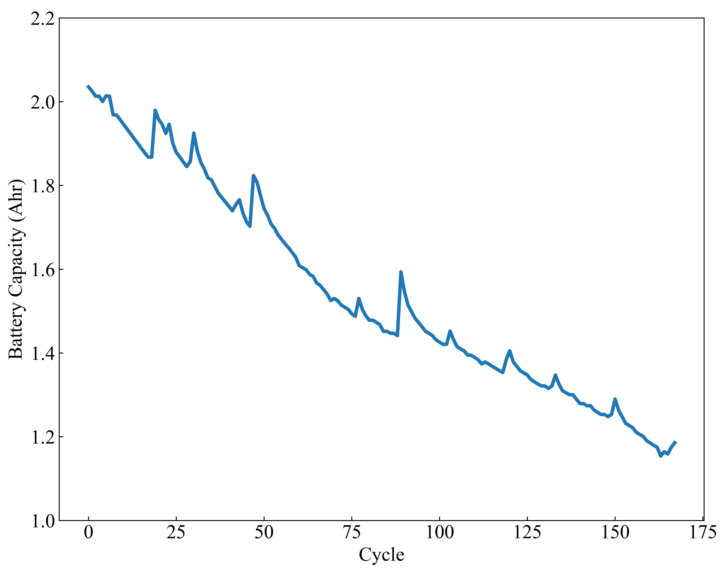The most intensively used model is the Wiener process, which is well-known due to its nice physical explanations and mathematical properties [7]. It owns the ability to describe a non-monotonic degradation evolution path, which makes itself distinct from other stochastic process models, such as the Gamma process and inverse Gaussian process. And this ability is indeed the expected trait when modeling the capacity loss of Li-ion batteries, as the capacity change with repeated charge-discharge cycles has a fluctuation characteristic, as shown in Figure 1. This figure depicts the capacity of battery $\#6$ with operational cycles based on the data set provided by [8]. Taking the Wiener process as a basic model, many research works have focused on the extensions that could improve model flexibility and applicability. One commonly used extension method is to consider a nonlinear drift parameter, which can be assumed in the form of an integral with a variable upper limit [9], a multi-stage function [10], and even a stochastic process [11]. At the same time, various filtering techniques can be incorporated with state-space-based prognostic models so that the parameters of degradation models can be updated sequentially with new observations [12,13,14]. Moreover, random effect and measurements error can be also involved in models to capture the heterogeneity of batteries and the variation caused by environmental factors or measurements [15,16]. Besides the Wiener process, the Gaussian process is another stochastic model that can be used for modeling the degradation of Li-ion batteries; see [17,18] for reference.

The methods discussed above can effectively describe the general decline trend for the capacity of batteries with operational cycles, but unfortunately, they do not sufficiently take into account the fact that the fluctuation represents not only the accumulative effect from numerous uncontrollable factors but also the capacity regeneration rooted in the Li-ion batteries. The capacity regeneration phenomenon, also called the relaxation phenomenon, is accounted for the self-recharge during the rest or relaxation period. When rest, battery cells are allowed to stand without passing a current through an external circuit. Then the reaction products that build up around the electrodes in cells would have a chance to dissipate, leading to an increase in the available capacity for the next cycle [19]. Many works have noticed the important role these occasionally considerable capacity changes play in degradation modeling and try to model the frequency and size of the changes mathematically. Zhai and Ye [20] and Shen et al. [21] introduced heavy-tailed non-normal measurement errors to capture the capacity regeneration by treating it as abnormal observation. However, this type of methods ignores that the regeneration indeed alters the degradation evolution of batteries. Saha and Geobel [19] considered the positive relationship between the self-charge and the rest period between two successive charge-discharge cycles and then modeled the capacity regeneration by an exponential process and estimated the RUL in the particle filter framework. Zhang et al. [22] regarded the capacity loss and regeneration as a stochastic switching working mode, and represented the mode by assuming piecewise functions for the drift coefficient of a diffusion model. Zhang et al. [23] used a random jump process to describe the capacity regeneration phenomenon and proposed a jump-diffusion model for RUL prediction.

Since the capacity regeneration distinguishes itself from the general decline trend by sudden and substantial jumps, it may be more efficient to separate capacity observations into different groups so that the general degradation trend and the capacity regeneration can be modeled respectively. Orchard et al. [24] presented and evaluated different methods for the detection of capacity regeneration phenomena in Li-ion batteries and developed the corresponding nonlinear, non-Gaussian state-space models. Qin et al. [25] adopted a support vector machine and hyperplane shift model to detect long rest time intervals and used Gaussian process and nonlinear models to describe the capacity loss and recovery. Xu et al. [26] identified the effective relaxation periods by comparing each period to a subject threshold and then developed a degradation model by modeling and combining three different modes that occur in capacity fade evolution.

Our paper also focuses on how to better describe the coexistence of capacity loss and regeneration and intends to model them separately with the help of a jump detection test. Enlightened by the similarity between the jumps in financial asset prices and the capacity regeneration of Li-ion batteries, we consider a jump-diffusion process model, of which the diffusion part is a geometric Brownian process and the jumps are assumed to follow an exponential distribution. The geometric Brownian process is well known as the Black-Scholes option pricing model and also provides another solution to deal with the nonlinearity in degradation modeling [27]. Based on the jump-diffusion process model, the nonparametric jump detection test proposed by Lee and Mykland (LM) [28] is adopted to identify the jump arrival times and then separate battery degradation data into two series, jump series and diffusion series. With the help of probabilistic programming, the Markov chain Monte Carlo (MCMC) sampling algorithm is utilized to estimate the parameters for the jump and diffusion parts of the degradation model, respectively. Moreover, distribution functions of failure time and residual useful life (RUL) are discussed. Simulation results show that the jump-diffusion model and the estimation method are feasible in modeling the battery capacity data and have a good performance in predicting the RUL.

The rest of the paper is organized as follows. Section 2 presents the formulation of the exponential jump-diffusion model. Section 3 presents the LM jump detection test, and also discusses the estimation of the model parameters and failure time/RUL distributions. Section 4 presents Monte Carlo simulations and the results. In Section 5, a Li-ion battery capacity data set is analyzed. Finally, Section 6 concludes the whole work.

2. Formulation of the Degradation Model

Let $Y_t$ denote the capacity of a Li-ion battery at time t. As usual, the degradation of this battery is the process $\{Y_t,t\ge 0\}$. Suppose that the degradation process follows a single exponential jump diffusion process model

$$d{Y}_t=Y_t(\mu dt+\sigma d{B}_t+[exp\left(X\right)-1]d{N}_t),t\ge 0,$$

(1)

where $\mu$ is the drift rate, $\sigma$ is the diffusion coefficient with $\sigma >0$, $B_t$ is the standard Brownian motion, $N_t$ is a homogeneous Poisson process with intensity $\lambda$, and X is an exponential distributed random variable with mean $1/\eta$, X∼$exp\left(\eta \right)$. Assume that $B_t$, $N_t$ and X are independent with each other. Applying Ito’s lemma on (1) yields

$$dlog{Y}_t=(\mu -\frac{1}{2}{\sigma }^2)dt+\sigma d{B}_t+Xd{N}_t,t\ge 0.$$

(2)

Further denoting $\nu =\mu -\frac{1}{2}{\sigma }^2$ and integrating the differential Equation (2) over $(0,t]$, we can obtain the solution to (1), i.e., the integral form of (1),

$$Y_t=Y_{0}exp(\nu t+\sigma B_t+\sum _{i=1}^{N_t}{X}_i),t\ge 0,$$

(3)

where $Y_0$ is the initial value, and $\nu$ is the drift rate for the logarithm of $Y_t$.

From (3), it is clear that the considered jump-diffusion model is based on the geometric Brownian motion, which corresponds to the general decline trend of capacity, and at the same time, includes a homogeneous compound Poisson process, which captures the occasionally occurred capacity regeneration. This setting implies that there exist two types of variation in the degradation model, of which the smaller one is from the diffusion process, while the larger one is incurred by the jump process.

As we know, the summation of random variables usually has complicated distribution functions, which would result in parameter estimation, a cumbersome job. Such a problem also exists in the model (3). Either the summation of $\sigma B_t$ and ${\sum }_{i=1}^{N_t}{X}_i$ or even ${\sum }_{i=1}^{N_t}{X}_i$ itself reminds us the difficulty of using traditional estimation methods, such as maximum likelihood estimation, when estimating the model parameters. A possible way to deal with this problem is to simplify the model (3) by approximating the compound Poisson jump process by a Bernoulli jump process, which was discussed by Ball and Torous [29,30]. To do so, we decompose (3) into a small time interval $(t,t+\Delta t)$,

$$\Delta log{Y}_t=\nu \Delta t+\sigma \Delta B_t+\sum _{i=1}^{\Delta N_t}{X}_i,t\ge 0,$$

(4)

where $\Delta log{Y}_t=log{Y}_{t+\Delta t}-log{Y}_t$, $\Delta B_t=B_{t+\Delta t}-B_t$ is the increment of the Brownian motion, and $\Delta N_t=N_{t+\Delta t}-N_t$ is the number of jumps that occur at $(t,t+\Delta t]$. Because the occurrence of capacity regeneration is not frequent during the entire measurement period, the Bernoulli jump process can be put forward as an appropriate model for capacity jumps. The distinguishing characteristic of the Bernoulli jump process is that over a fixed period of time, either no self-recharge impacts upon the capacity change or the regeneration occurs at most once. Moreover, Ball and Torous [30] showed that, as the time interval gets smaller, the Bernoulli process would converge to the Poisson process. Because of the simple structure and nice properties of the Bernoulli jump process, we assume that during the small time interval $(t,t+\Delta t)$ there is at most one jump, and the jump occurs with a probability $\lambda \Delta t$. That is,

$$P\left(\sum _{i=1}^{\Delta N_t}{X}_i=X_1\right)=\lambda \Delta t,P\left(\sum _{i=1}^{\Delta N_t}{X}_i=0\right)=1-\lambda \Delta t.$$

Then $\Delta log{Y}_t$ in (4) can be simplified as

$$\Delta log{Y}_t=\nu \Delta t+\sigma \Delta B_t+Z_t{X}_t,t\ge 0,$$

(5)

where $Z_t$ is a Bernoulli random variable with $P(Z_t=1)=\lambda \Delta t$, $P(Z_t=0)=1-\lambda \Delta t$, and $X_t$ is the jump size subject to the exponential distribution with mean $1/\eta$, $X_t$∼$exp\left(\eta \right)$.

3. Parameter Estimation and RUL Prediction

To avoid computing the density function of $\sigma \Delta B_t+Z_t{X}_t$ in (5), we use the LM jump detection test together with the MCMC algorithm for estimating parameters instead of those traditional estimation methods.

3.1. LM Jump Detection Test

The LM jump detection test adopted in this paper is proposed by Lee and Mykland [28] with the original aim to identify jump arrival times in financial asset prices. This test is a nonparametric test and refers to a single test at a certain time without assuming whether there were or were no jumps before or after that time. If the detection of jumps over time is expected, taking single tests over available times would work for the purpose.

Suppose that there is a fixed time horizon T, and n is the number of observations in $[0,T]$. Observations of $Y_t$, equivalently $log{Y}_t$, occurs at discrete times $0=t_0<t_1<\dots <t_n=T$. The time interval between two successive observations is $\Delta t_i=t_i-t_{i-1}$. For simplicity, assume $\Delta t_i=\Delta t=T/n$, i.e., observation times are equally spaced.

To determine whether there was a jump that arrived at $t_i$, the LM test considers a local movement of the jump-diffusion process within a predetermined window size K. Based on the previous $K-1$ observations just before the testing time $t_i$, the test statistics $\mathcal{L}\left(i\right)$ is defined as

$$\mathcal{L}\left(i\right)=\frac{log{Y}_{t_i}/Y_{t_{i-1}}-{\widehat{m}}_i}{\widehat{\sigma \left(t_i\right)}},$$

(6)

where

$${\widehat{m}}_i=\frac{1}{K-1}\sum _{j=i-K+1}^{i-1}(log{Y}_{t_j}/Y_{t_{j-1}}),$$

(7)

$$\widehat{\sigma {\left(t_i\right)}^2}=\frac{1}{K-2}\sum _{j=i-K+2}^{i-1}|log{Y}_{t_j}/Y_{t_{j-1}}\left|\right|log{Y}_{t_{j-1}}/Y_{t_{j-2}}|.$$

(8)

Note that ${\widehat{m}}_i$ is the average of the logarithmic change rate of $Y_t$ in the window and used to estimate the change rate at the time $t_i$. And $\widehat{\sigma {\left(t_i\right)}^2}$, called realized bipower variation in [28], is a consistent estimator for the local variation only from the diffusion part of the process. The work [28] showed in Lemma 1 that, with some conditions, as $\Delta t\to 0$,

$$\frac{{max}_{i\in {\overline{A}}_n}\left|\mathcal{L}\left(i\right)\right|-C_n}{S_n}\to \xi ,$$

(9)

where $\xi$ has a cumulative distribution function $P(\xi \le x)=exp(-e^{-x})$, ${\overline{A}}_n$ is the set of $i\in \{1,2,\dots ,n\}$ so that there is no jump in $(t_{i-1},t_i]$,

$$C_n=\frac{{(2logn)}^{1/2}}{c}-\frac{log\pi +log(logn)}{2c{(2logn)}^{1/2}}\mathrm{and}{S}_n=\frac{1}{c{(2logn)}^{1/2}},$$

where $c=\sqrt{2}/\sqrt{\pi }\approx 0.7979$.

Given a significance level $\alpha$, the LM test selects the $1-\alpha$ percentile of the distribution of $\xi$ as the threshold for $\frac{\left|\mathcal{L}\left(i\right)\right|-C_n}{S_n}$. In this paper, we set $\alpha =0.01$. Then the threshold ${\beta }^{*}$ satisfies $P(\xi \le {\beta }^{*})=exp(-e^{-{\beta }^{*}})=0.99$, which is equivalently ${\beta }^{*}=-log(-log\left(0.99\right))=4.6001$. Hence, the null hypothesis of no jump at $t_i$ is reject if $\frac{\left|\mathcal{L}\left(i\right)\right|-C_n}{S_n}>4.6001$.

Applying the above LM jump detection test over time, we can separate the n observation times into two sets, one for the time points at which the test declares the presence of a jump and the other for the time points at which no jump is detected. We denote the two sets by $B_n$ and $B_n^C$, respectively. Correspondingly, the observations also can be classified as either belonging to the jump series or to the non-jump/diffusion series. Let $S_i=log{Y}_{t_i}/Y_{t_{i-1}}$, $i=1,2,\dots ,n$. We can denote the jump series by ${\mathit{S}}^{J_0}=\{S_i,i\in B_n\}$, and the diffusion series by ${\mathit{S}}^{C_0}=\{S_i,i\in B_n^C\}$.

Remark 1.

Note that the test statistic in (6) is not applicable for the first $K-1$ observation times, $t_1,\dots ,t_{K-1}$. When applying the LM test at these times, we narrow down the window size to $i-1$, $i=1,\dots ,K-1$. That means to use all observations before $t_i$ to compute the statistic. Other alternative ways to deal with the problem can be assuming no jump is detected at these times or excluding the corresponding observations from parameter estimation, etc.

3.2. Parameter Estimation Based on MCMC Algorithm

To estimate the parameter $\theta ={(\nu ,\sigma ,\lambda ,\eta )}^{\prime }$ in the model (5), we need to expand the diffusion series ${\mathit{S}}^{C_0}$ to accommodate all observation times by interpolating values at all detected jump arrival times $B_n$. For $i\in B_n$, the latent observation from the diffusion part, denoted by $S_i^{\prime }$, can be given via the moving average algorithm,

$$S_i^{\prime }=\left\{\begin{array}{cc}(S_1+S_2+\dots +S_b)/b\hfill & i\le b\\ (S_{i-b}+S_{i-b+1}+\dots +S_{i-1})/b\hfill & i>b\end{array},\right.$$

(10)

where b is a predetermined lag. For $i\in B_n^C$, simply let $S_i^{\prime }=S_i$. Then we can have a modified diffusion series ${\mathit{S}}^C=\{S_i^{\prime },i=1,2,\dots ,n\}$. And the difference between $S_i$ and $S_i^{\prime }$ can be assigned as the jump size at each jump arrival time. Let $J_i=S_i-S_i^{\prime }$. Then a modified jump series ${\mathit{S}}^J=\{J_i,i\in B_n\}$ is obtained. Based on these two modified series, an initial estimator for $\theta$ can be derived. We denote it by ${\widehat{\theta }}_{\mathrm{LM}}$, as it is a by-product of the LM jump detection test. It is also referred to as the estimator based on the LM method in the following.

As the Wiener process has independent and stationary increments that are normally distributed, the increments from the diffusion part of (5) follow a normal distribution with mean $\nu \Delta t$ and variance ${\sigma }^2\Delta t$,

$$(log{Y}_{t_i}-Z_{t_i}{X}_{t_i})-(log{Y}_{t_{i-1}}-Z_{t_{i-1}}{X}_{t_{i-1}})=\nu (t_i-t_{i-1})+\sigma (B_{t_i}-B_{t_{i-1}})\stackrel{\mathrm{i}.\mathrm{i}.\mathrm{d}}{\sim }N(\nu \Delta t,{\sigma }^2\Delta t),i=1,\dots ,n.$$

(11)

As the diffusion series ${\mathit{S}}^C$ represents the increments from the diffusion part (11), nature estimators for the drift rate $\nu$ and the squared diffusion coefficient ${\sigma }^2$ are given by

$$\begin{array}{ccc}\hfill {\widehat{\nu }}_{\mathrm{LM}}& =& \frac{1}{n\Delta t}{\overline{S}}^{\prime },\hfill \end{array}$$

(12)

$$\begin{array}{ccc}\hfill {\widehat{{\sigma }^2}}_{\mathrm{LM}}& =& \frac{1}{(n-1)\Delta t}\sum _{i=1}^n{(S_i^{\prime }-{\overline{S}}^{\prime })}^2,\hfill \end{array}$$

(13)

where ${\overline{S}}^{\prime }={\sum }_{i=1}^n{S}_i^{\prime }/n$ is the average of the diffusion series ${\mathit{S}}^C$. And ${\widehat{\sigma }}_{\mathrm{LM}}=\sqrt{{\widehat{{\sigma }^2}}_{\mathrm{LM}}}$.

For the jump part, an estimator for the intensity $\lambda$ of the homogeneous Poisson process is

$${\widehat{\lambda }}_{\mathrm{LM}}=\frac{n_J}{n\Delta t},$$

(14)

where $n_J$ is the number of elements in $B_n$ or the number of detected jump arrival times. And the parameter for exponential jump $\eta$ can be estimated by

$${\widehat{\eta }}_{\mathrm{LM}}=\frac{n_J}{{\sum }_{i=1}^{n_J}{J}_i},$$

(15)

That is the reciprocal of the mean jump size, which is obtained by averaging the jump series ${\mathit{S}}^J$.

With the initial estimator ${\widehat{\theta }}_{\mathrm{LM}}={({\nu }_{\mathrm{LM}},{\sigma }_{\mathrm{LM}},{\lambda }_{\mathrm{LM}},{\eta }_{\mathrm{LM}})}^{\prime }$, we further adopt the MCMC sampling algorithm to obtain a more accurate estimator for $\theta$. The MCMC sampling algorithm is carried out with the help of probabilistic programming, which is an emerging branch in statistical learning and can be implemented with the Python package-PyMC3 [31,32]. PyMC3 is an open source framework and features several MCMC sampling techniques, such as the Metropolis-Hastings sampler, the No-U-Turn Sampler (NUTS) [33], and Hamiltonian Monte Carlo [34], etc. Here the Metropolis-Hastings sampler is used to randomly updates the values of parameters. Another alternative is the NUTS, which may speed up the sampling procedure for continuous random variables.

Probabilistic programming aims for flexible and automatic Bayesian inference. Thus a suitable Bayesian statistical model should be developed for further parameter estimation. Suppose that the degradation process follows the simplified jump-diffusion model $\left(5\right)$, and the parameters in the model are also subject to some probability distributions, i.e., prior distributions. For convenience, conjugate priors are chosen. For the diffusion part that is dominated by a normal distribution, the parameters $\nu$ and $\sigma$ have the priors,

$$\nu \sim N({\mu }_{\nu },{\sigma }_{\nu }^2),{\sigma }^2\sim \mathrm{Inverse}\mathrm{Gamma}({\alpha }_{{\sigma }^2},{\beta }_{{\sigma }^2}).$$

(16)

In the jump part, the assumption of Bernoulli distribution for $Z_t$ and exponential distribution for $X_t$ implies that the priors for $\lambda$ and $\eta$ can be

$$\lambda \sim \mathrm{Beta}({\alpha }_{\lambda },{\beta }_{\lambda }),\eta \sim \mathrm{Gamma}({\alpha }_{\eta },{\beta }_{\eta }).$$

(17)

The parameters of the priors can be set such that the means of the prior distributions equal or approximately equal the LM estimate ${\widehat{\theta }}_{\mathrm{LM}}$.

The procedure of the MCMC sampling and further estimation given the priors is as follows, which can be carried out in two steps.

Step 1

Estimation of $\nu$ and $\sigma$. Based on the diffusion part $\nu \Delta t+\sigma \Delta B_t$ with the priors (16) and the modified diffusion series ${\mathit{S}}^C$,

• Generate M Markov chains with length Q for both $\nu$ and $\sigma$;
• Discard the first $Q_0$ samples for burn-in in each of the $2M$ chains;
• For each parameter, diagnose the convergence of Markov chains by Gelman–Rubin variance ratio test based on the M chains;
• For each parameter, compute the sample mean and sample variance of the remaining $M\times (Q-Q_0)$ samples.

From Step 1, the two obtained sample means are taken as the final estimates for $\nu$ and $\sigma$, denoted by $\widehat{\nu }$ and $\widehat{\sigma }$. And the square roots of sample variances are the empirical standard errors for $\widehat{\nu }$ and $\widehat{\sigma }$. Next, we estimate the other two parameters $\lambda$ and $\eta$.

Step 2

Estimation of $\lambda$ and $\eta$. Based on the simplified model $\left(5\right)$ with the priors (17), the original series $\{S_i,=1,\dots ,n\}$ and the estimates $\widehat{\nu }$, $\widehat{\sigma }$ obtained in Step 1,

• Generate M Markov chains with length Q for both $\lambda$ and $\eta$;
• The same as Step 1–2;
• The same as Step 1–3;
• The same as Step 1–4.

Similarly, the sample means obtained from the above Steps 2–4 are regarded as the final estimates for $\lambda$ and $\eta$, denoted by $\widehat{\lambda }$ and $\widehat{\eta }$. And the square roots of sample variances are also the empirical standard errors for $\widehat{\lambda }$ and $\widehat{\eta }$.

In both steps, we arbitrarily choose $M=2$, $Q=5500$, and $Q_0=500$. This means that all estimates are computed based on $2\times (5500-500)=$ 10,000 samples. The final estimate for $\theta$ is $\widehat{\theta }={(\widehat{\nu },\widehat{\sigma },\widehat{\lambda },\widehat{\eta })}^{\prime }$. This estimation is referred to be based on the combined method as the LM test and the MCMC method are involved.

3.3. RUL Prediction

For an in-use product, a so-called soft failure is considered to occur when the degradation process reaches a prescribed threshold of D. Apparently, the threshold for Li-ion batteries can be set as a certain value between $70\%$ and $80\%$ of rated capacity. Under this failure concept, the failure time of a Li-ion battery is defined as the first passage time $T_D$ of the degradation process, which is a random variable with the expression

$$T_D=inf\{t:Y_t\le D|Y_0>D\}.$$

(18)

In addition, the RUL is a conditional random variable derived from the failure time and has different forms for different purposes. If we concern the RUL of a population, the RUL at time t can be defined as

$$L_D^1\left(t\right)=T_D-t|T_D>t.$$

(19)

If we are interested in a particular battery with observed true degradation data $\mathit{y}=(y_1,\dots ,y_n)$ at $\mathit{t}=(t_1,\dots ,t_n)$, the RUL at time $t_n$ can be better given by

$$L_D^2\left(t_n\right)=inf\{t:Y_{t_n+t}\le D|y_0>D,y_1>D,\dots ,y_n>D\}.$$

(20)

In our jump-diffusion model, the Wiener process and the homogeneous Poisson process own the Markov property, and both are assumed to be independent of the jump size. Thus $L_D^2\left(t_n\right)$ is actually equivalent to the first passage time to the threshold $D-y_n$. That is, $L_D^2\left(t_n\right)$ has a same distribution as $T_{D-y_n}$, i.e., $L_D^2\left(t_n\right)\stackrel{\mathrm{d}}{=}{T}_{D-y_n}$.

If the degradation $\{Y_t,t\ge 0\}$ is a Wiener process $Y_t=\nu t+\sigma B_t$, the first passage time follows a inverse Gaussian distribution, $T_D\sim \mathrm{IG}(D/\nu ,D/{\sigma }^2)$. However, our model in (4) or (5) involves an extra jump process, which makes the inverse Gaussian distribution not directly applicable. Instead, we use the Monte Carlo simulation method to approximate the distributions of the failure time and RULs. The approximation method takes the following steps:

• Based on the model (5) and the parameter estimate $\widehat{\theta }$, generate R degradation paths, each composed of n observations at $t_1,\dots ,t_n$. Denote these R path by ${\mathit{y}}^r=(y_1^r,\dots ,y_n^r)$, $r=1,\dots ,R$.
• For a given threshold D, record the first passage time to D for each degradation path. Denote these times by $t_D^r$, $r=1,\dots ,R$.
• Based on $t_D^r$, $r=1,\dots ,R$, calculate the empirical cumulative distribution function (CDF) ${\widehat{F}}_R\left(t\right)$ and the mean ${\overline{t}}_{D,R}$.
• For a given time $t^{*}$, screen out those first passage times great than $t^{*}$, denoted by $t_D^{*r}$, $r=1,\dots ,R^{*}$. With $\{t_D^{*r}-t^{*}\}$, calculate the empirical CDF ${\widehat{G}}_{R^{*}}\left(t\right)$ and the mean ${\overline{t}}_{D,R^{*}}^{*}$.

Obviously, the empirical CDFs ${\widehat{F}}_R\left(t\right)$ and ${\widehat{G}}_{R^{*}}\left(t\right)$ are approximations for the CDFs of the failure time $T_D$ and RUL $L_D^1\left(t^{*}\right)$. That is

$$\begin{array}{c}\hfill \widehat{F_{T_D}}\left(t\right)={\widehat{F}}_R\left(t\right),\widehat{F_{L_D^1\left(t^{*}\right)}}\left(t\right)={\widehat{G}}_{R^{*}}\left(t\right),t\ge 0.\end{array}$$

(21)

At the same time, the probability density functions (PDFs) of $T_D$ and $L_D^1\left(t^{*}\right)$ can be estimated by the empirical PDFs, denoted by $\widehat{f_{T_D}}\left(t\right)$ and $\widehat{f_{L_D^1\left(t^{*}\right)}}\left(t\right)$. And the expectation of $T_D$ and $L_D^1\left(t^{*}\right)$, named mean time to failure and mean residual useful life (MRUL), can be estimated by ${\overline{t}}_{D,R}$ and ${\overline{t}}_{D,R^{*}}^{*}$. In fact, with the R first passage times, the estimates of various quantiles of $T_D$ and $L_D^1\left(t^{*}\right)$ also can be obtained. In order to guarantee the accuracy of the estimation, the number of R can be chosen as large enough. Here we set $R=5000$.

4. Simulation Study

4.1. The Choice of the Parameters and the Performance of the Estimation Methods

A simple Monte Carlo simulation experiment is conducted to evaluate the performance of the adopted estimation methods and facilitate further real data analysis. The data are generated based on the original diffusion-jump process (4) with the drift rate $\nu =-0.05$, the diffusion coefficient $\sigma =0.005$, the Poisson intensity $\lambda =0.05$, and the exponential parameter $\eta =20$. In the simulation study, we assume that the degradation signal of a product is measured at 200 time points, $t={(1,\dots ,200)}^{\prime }$, and $\Delta t=1$. This set of parameters mimics the capacity data that will be analyzed in the next section. In this experiment, 200 replications are run.

To choose suitable values for the window size K in the LM test and the lag b in the smoothing average, we evaluate the performance of the initial estimator ${\widehat{\theta }}_{\mathrm{LM}}$ for various combinations of K and b, with K ranging from 5 to 15 and b from 3 to 10.

Table 1. The estimation results of ${\widehat{\theta }}_{\mathrm{LM}}$ for different $(K,b)$’s: mean (rmse).

		$\mathit{K}=8$	$\mathit{K}=9$	$\mathit{K}=10$	$\mathit{K}=11$
$b=5$	$\nu$	−0.0047	−0.0047	−0.0047	−0.0047
		(0.0005)	(0.0005)	(0.0005)	(0.0004)
	$\sigma$	0.0054	0.0054	0.0054	0.0054
		(0.0008)	(0.0007)	(0.0008)	(0.0006)
	$\lambda$	0.0297	0.0297	0.0295	0.0294
		(0.0236)	(0.0238)	(0.0238)	(0.0240)
	$\eta$	20.083	19.181	18.721	18.655
		(6.997)	(5.382)	(4.9883)	(5.2900)
$b=6$	$\nu$	−0.0047	−0.0047	−0.0047	−0.0047
		(0.0005)	(0.0005)	(0.0004)	(0.0004)
	$\sigma$	0.0054	0.0054	0.0054	0.0054
		(0.0008)	(0.0007)	(0.0007)	(0.0006)
	$\lambda$	0.0299	0.0298	0.0296	0.0294
		(0.0234)	(0.0237)	(0.0238)	(0.0240)
	$\eta$	20.386	19.682	18.704	18.605
		(7.2857)	(6.2454)	(4.9247)	(5.2474)
$b=7$	$\nu$	−0.0047	−0.0047	−0.0047	−0.0047
		(0.0005)	(0.0005)	(0.0004)	(0.0004)
	$\sigma$	0.0054	0.0054	0.0054	0.0054
		(0.0008)	(0.0007)	(0.0007)	(0.0006)
	$\lambda$	0.0299	0.0297	0.0296	0.0295
		(0.0234)	(0.0238)	(0.0238)	(0.0239)
	$\eta$	20.172	19.2022	18.732	18.727
		(7.0741)	(5.3714)	(4.9631)	(5.2456)

reports the empirical mean and root-mean-square error (rmse) of the estimated parameters ${\widehat{\theta }}_{\mathrm{LM}}$. Only part of the simulation results are given here due to the limited space of this paper. The results in Table 1 show that the impact of $(K,b)$ on ${\widehat{\nu }}_{\mathrm{LM}}$ and ${\widehat{\sigma }}_{\mathrm{LM}}$ is negligible, and relatively little on ${\widehat{\lambda }}_{\mathrm{LM}}$, but rather noticeable on ${\widehat{\eta }}_{\mathrm{LM}}$. The emergence of the phenomenon is not strange because the detection of jumps and the estimation of jump size heavily depend on K and b. A comparison reveals that ${\widehat{\eta }}_{\mathrm{LM}}$ has the smallest rmse when $K=10$ and $b=6$. Thus $(K,b)$ is set as $(10,6)$ in further study for the simulated model as well as the capacity data analysis.

Following the principles of simplicity and the distribution means close to ${\widehat{\theta }}_{\mathrm{LM}}$, the priors for the four parameters are set as follows through trial and error,

$$\begin{array}{cc}\hfill & \nu \sim N({\widehat{\nu }}_{\mathrm{LM}},100),{\sigma }^2\sim \mathrm{Inverse}\mathrm{Gamma}(1/{\widehat{\sigma }}_{\mathrm{LM}},{\widehat{\sigma }}_{\mathrm{LM}}),\\ & \lambda \sim \mathrm{Beta}(2,2/{\widehat{\lambda }}_{\mathrm{LM}}),\eta \sim \mathrm{Gamma}(0.5{\widehat{\eta }}_{\mathrm{LM}},0.5).\end{array}$$

(22)

Figure 2 and

Table 2. The estimation results in one replication: mean [se].

	$\mathit{\nu }$	$\mathit{\sigma }$	$\mathit{\lambda }$	$\mathit{\eta }$
LM	−0.0049	0.0048	0.0350	16.6958
Combined	−0.0049	0.0048	0.0423	18.6473
	[0.0004]	[0.0001]	[0.0184]	[6.0570]

show the parameter estimation results in one of the 200 replications. From Figure 2, we observe the estimated kernel density functions for $\widehat{\nu }$, $\widehat{\sigma }$, $\widehat{\lambda }$, and $\widehat{\eta }$, respectively. For each parameter, two kernel density functions are presented, in the dotted line and solid line, which are estimated from the two realized Markov chains generated by the MCMC method. And the average of the means of the two density functions is taken as the parameter estimate obtained in this replication. At the same time, the realized Markov chains, two for each parameter, are plotted in the right panel, which visually displays the quick convergence of the chains and thus indicates the validity of the MCMC algorithm. The convergence are further verified by the Gelman and Rubin convergence diagnostic, as the corresponding statistic takes value 1 for all the four parameters. Moreover, Table 2 compares the performances of ${\widehat{\theta }}_{\mathrm{LM}}$ and $\widehat{\theta }$ in one replication. It is clear that the utilization of the MCMC algorithm indeed improves the accuracy of parameter estimation and could provide the empirical standard error (se) to measure the variability of $\widehat{\theta }$.

Similar conclusions can be achieved from the results in

Table 3. The comparison between the LM estimation and combined estimation methods.

	LM				Combined
	Mean	rmse	se	MAPE	Mean	rmse	se	MAPE
$\nu$	−0.0047	0.0004	0.0004	0.0708	−0.0047	0.0005	0.0004	0.0736
$\sigma$	0.0054	0.0007	0.0006	0.0957	0.0053	0.0004	0.0003	0.0514
$\lambda$	0.0296	0.0238	0.0121	0.4269	0.0401	0.0119	0.0030	0.2085
$\eta$	18.704	4.9247	4.7511	0.1972	20.569	1.5733	1.3724	0.0784

, which summarizes the empirical mean, se, rmse, and mean absolute percentage error (MAPE) of the parameter estimates. The MAPE for $\widehat{\theta }$ is defined as $\mathrm{MAPE}(\widehat{\theta })=\frac{1}{L}{\sum }_{l=1}^L|{\widehat{\theta }}_l/{\theta }_0-1|\times 100\%$, where ${\theta }_0$ is the true parameter, L is the number of replications and set as 200 in our experiment, and ${\widehat{\theta }}_l$ is the estimate obtained in the lth replication. The results in the table clearly show that the estimator based on the combined method $\widehat{\theta }$ has a smaller bias, se, rmse, and MAPE than the initial one ${\widehat{\theta }}_{\mathrm{LM}}$.

Remark 2.

In Figure 2, the kernel density estimates for the parameters λ and η are highly skewed. This is due to the setting of the two corresponding priors, which have long right tails. However, a close examination on the results from the 200 replications shows that, the samples with values larger than $2\lambda$ and $2\eta$ take only about $6\%$ and $2\%$ out of 10,000 MCMC samples in average.

To further demonstrate the superiority of the combined estimation method, we compare the performances of failure time and RUL prediction based on the two estimation methods. For the failure time $T_D$, both the true and the estimated PDFs are computed by the Monte Carlo method given in Section 3.3, and compared in terms of the Jensen-Shannon divergence. That is, if we denote the true parameter by ${\theta }_0$,

$$JS(\widehat{f_{T_D}}(t;{\theta }_0)\Vert \widehat{f_{T_D}}(t;\widehat{\theta }))=\frac{1}{2}KL\left(\widehat{f_{T_D}}(t;{\theta }_0)\Vert \frac{\widehat{f_{T_D}}(t;{\theta }_0)+\widehat{f_{T_D}}(t;\widehat{\theta })}{2}\right)+\frac{1}{2}KL\left(\widehat{f_{T_D}}(t;\widehat{\theta })\Vert \frac{\widehat{f_{T_D}}(t;{\theta }_0)+\widehat{f_{T_D}}(t;\widehat{\theta })}{2}\right),$$

(23)

where ${\theta }_0$ is the true parameter, $\widehat{\theta }$ is the parameter estimate, and KL is the Kullback–Leibler divergence that measures the similarity between two PDFs, say $P_1$ and $P_2$, and defined as

$$KL(P_1\Vert P_2)={\int }_{-\infty }^{\infty }{P}_{1}log(P_1/P_2)dt.$$

(24)

For both JS divergence and KL divergence, small values are expected as they indicate a good estimation of the PDF.

For the RUL, the expectation MRUL is used for estimation and comparison. Given a arbitrary time $t^{*}=25$, we are interested in its MRUL, $\mathrm{MRUL}\left(25\right)=E\left[L_D^1\left(25\right)\right]$. As shown in Section 3.3, the estimate $\widehat{\mathrm{MRUL}}\left(25\right)$ is the average of the first passage times greater than 25, which are obtained from 5000 generated paths given the parameter estimate $\widehat{\theta }$. The performance of the MRUL estimate is measured by the MAPE to the real MRUL, $\mathrm{MAPE}(\widehat{\mathrm{MRUL}}\left(25\right))=\frac{1}{L}{\sum }_{l=1}^L|\widehat{\mathrm{MRUL}}\left(25\right)/\mathrm{MRUL}\left(25\right)-1|\times 100\%$, where $L=200$ and $\mathrm{MRUL}\left(25\right)$ is also approximated by the Monte Carlo simulation method but with the true parameter ${\theta }_0$.

Table 4. The results for the failure rate and RUL prediction.

	LM	Combined
JS: $f_{T_D}\left(t\right)$	0.0085	0.0003
	[0.0314]	[0.0003]
MAPE: MRUL$\left(25\right)$	0.3990	0.0524

summarizes the empirical mean and se of the JS divergence as well as the MAPE based on the two estimation methods. It is clear that the combined method provides much better performances than the LM method when predicting both the failure time and RUL. This conclusion is also supported by Figure 3, in which the estimated PDF of $T_D$ by the combined method (red line) is closer to the true one (blue line).

4.2. A Brief Discussion on Model Misspecification

To better understand the robustness of the considered model together with the estimation procedure, we further investigate their performances under model misspecification. An additional simulation experiment is carried out with the data generated from a new jump-diffusion process, which remains with the geometric Brownian process as the base model but assumes normal-distributed jumps. The assumption of the normal-type jumps was also considered in Zhang et al. [35], but their model was built on the nonlinear Weiner process.

In the data generating process, we let the jump size $X_t$ follow a normal distribution with mean $0.05$ and standard deviation $0.01$, $X_t$∼$N(0.05,{0.01}^2)$, which has the same mean as the exponential jump considered in the previous. The setting of other parameters is the same as in the previous experiment. That is, the drift rate $\nu =-0.05$, the diffusion coefficient $\sigma =0.005$, and the Poisson intensity $\lambda =0.05$. Moreover, the degradation signal of a product is also assumed to be measured at 200 time points, $t={(1,\dots ,200)}^{\prime }$, and $\Delta t=1$. In this experiment, 200 replications are run.

The generated data are fitted by our target model (5) with the estimation methods discussed in Section 3.

Table 5. The estimation results of ${\widehat{\theta }}_{\mathrm{LM}}$ for different $(K,b)$’s: mean (se), normal jumps.

		$\mathit{K}=8$	$\mathit{K}=9$	$\mathit{K}=10$	$\mathit{K}=11$	$\mathit{K}=12$
$b=5$	$\nu$	−0.0049	−0.0049	−0.0048	−0.0048	−0.0048
		(0.0004)	(0.0004)	(0.0004)	(0.0004)	(0.0004)
	$\sigma$	0.0054	0.0055	0.0055	0.0055	0.0056
		(0.0008)	(0.0009)	(0.0009)	(0.0009)	(0.0009)
	$\lambda$	0.0473	0.0468	0.0465	0.0463	0.0460
		(0.0138)	(0.0142)	(0.0139)	(0.0139)	(0.014)
	$\eta$	21.934	21.474	21.222	21.041	21.041
		(4.6436)	(2.9949)	(2.5277)	(2.1720)	(2.1923)
$b=6$	$\nu$	−0.0049	−0.0048	−0.0048	−0.0048	−0.0048
		(0.0004)	(0.00041)	(0.0004)	(0.0004)	(0.0004)
	$\sigma$	0.0054	0.0055	0.0055	0.0055	0.0056
		(0.0008)	(0.0009)	(0.0009)	(0.0009)	(0.0009)
	$\lambda$	0.0472	0.0467	0.0464	0.0463	0.0460
		(0.0138)	(0.0142)	(0.0139)	(0.0139)	(0.0140)
		21.732	21.442	21.156	21.022	21.022
		(3.8271)	(2.9743)	(2.4685)	(2.1296)	(2.1590)
$b=7$	$\nu$	−0.0049	−0.0049	−0.0048	−0.0048	−0.0048
		(0.0004)	(0.0004)	(0.0004)	(0.0004)	(0.0004)
	$\sigma$	0.0054	0.0055	0.0055	0.0055	0.0056
		(0.0008)	(0.0009)	(0.0009)	(0.0009)	(0.0009)
	$\lambda$	0.0472	0.468	0.0465	0.0463	0.0461
		(0.0138)	(0.0143)	(0.0139)	(0.0139)	(0.0140)
	$\eta$	21.707	21.416	21.140	21.015	21.011
		(3.6583)	(2.8687)	(2.4438)	(2.1477)	(2.1624)

reports the empirical mean and se of the estimated parameters ${\widehat{\theta }}_{\mathrm{LM}}$ for different combinations of K and b, with K ranging from 5 to 15 and b from 8 to 12. It is worthy noting that the se, instead of the rmse, is used in the table, because no rmse is available for $\eta$ due to the normal assumption for the jump size. The results in the table indicate that the recommended combination $(K,b)$ is changed to $(11,6)$ in this experiment for model misspecification.

Table 6. The comparison between the LM and combined estimation methods: normal jumps.

	LM				Combined
	Mean	rmse	se	MAPE	Mean	rmse	se	MAPE
$\nu$	−0.0048	0.0005	0.0004	0.0716	−0.0049	0.0004	0.0004	0.0668
$\sigma$	0.0055	0.0013	0.0009	0.1709	0.0052	0.0009	0.0008	0.0978
$\lambda$	0.0463	0.0164	0.0139	0.2555	0.0633	0.0262	0.0226	0.4158
$\eta$	21.022	-	2.1296	-	22.177	-	1.6105	-

No rmse and MAPE for η are due to the normal assumption for the jump size.

presents the parameter estimation results for ${\widehat{\theta }}_{\mathrm{LM}}$ and $\widehat{\theta }$, which are obtained from the 200 replications and with the same prior distributions given in (22). It is shown that the utilization of the MCMC algorithm improves the accuracy of the estimation for $\nu$ and $\sigma$, but fails to do so for $\lambda$. The reason for the opposite performances is that the fitted model and the data generating process differ in the distribution of jump size, which would distort the estimation for the parameters of the jump process. But overall, the estimation methods can give relatively satisfactory estimates for the parameters when the model is misspecified.

Table 7. The results for the failure rate and RUL prediction: normal jumps.

	LM	Combined
JS: $f_{T_D}\left(t\right)$	0.0035	0.0025
	[0.0044]	[0.0013]
MAPE: MRUL$\left(25\right)$	0.3898	0.2956

summarizes the empirical mean and se of the JS divergence for $\widehat{f_{T_D}}\left(t\right)$ and the MAPE for $\widehat{\mathrm{MRUL}}\left(25\right)$ respectively. It is observed that even under model specification, the combined estimation method still has better performances than the LM method for the prediction of both the failure time and RUL, although the improvement is not as significant as that in Table 4. Finally, we may conclude that, to some extent, the adopted model, together with the estimation procedure, can deal with the model specification problem.

5. Capacity Data Analysis

Here we revisit the capacity data of the Li-ion battery $\#6$ mentioned in Section 1. The Li-ion battery $\#6$ is a 18,650-sized rechargeable cell with LiNi${}_{0.8}$Co${}_{0.15}$Al${}_{0.05}$O${}_2$ cathode and graphite anode and was run through repeated charge and discharge cycles at room temperature (24 ${}^{°}$C). Charging was carried out in a constant current mode at $1.5$ A until the battery voltage reached $4.2$ V and then switched to a constant voltage mode until the charge current dropped to 20 mA. For the discharge, a constant current with a level 2 A was applied to the battery until the battery voltage fell to $2.5$ V. The experiment was stopped when the battery capacity faded from 2 Ahr to $1.4$ Ahr, a $30\%$ loss compared to the rated capacity. During each of the total 168 cycles, the battery capacity was measured by impedance measurement, which was executed through an electrochemical impedance spectroscopy frequency sweep from $0.1$ Hz to 5 kHz.

Denote by $Y_t$ the capacity at cycle t and by $S_t=log{Y}_t/Y_{t-1}$ the logarithm of the change rate of capacity, $t=1,\dots ,168$. A quick calculation tells that for $S_t$’s, the sample skewness and kurtosis are $3.9080$ and $24.934$, respectively. This indicates that $S_t$ follows an asymmetric and fat-tail distribution and undoubtedly cannot be modeled by a normal distribution. The non-normality of $S_t$’s further denies the geometric Brownian process as an underlying degradation model for $\left\{Y_t\right\}$. But after applying the LM jump detection test on $S_t$ over the 168 time points, we can get a diffusion series whose sample skewness and kurtosis become $-0.4015$ and $5.2576$. Although these two coefficients still slightly differ from 0 and 3, the skewness and kurtosis for normal distribution, they indeed give strong support for the feasibility of including a jump process into the degradation model. Hence it should be proper to adopt the jump-diffusion model (3) for describing the capacity data.

Based on (3), the unknown parameter $\theta ={(\nu ,\sigma ,\lambda ,\eta )}^{\prime }$ are estimated by the two methods, the LM method and the combined method. The priors are set as (22). The corresponding estimates ${\widehat{\theta }}_{\mathrm{LM}}$ and $\widehat{\theta }$ are listed in

Table 8. The parameter estimates are based on the two estimation methods.

	$\mathit{\nu }$	$\mathit{\sigma }$	$\mathit{\lambda }$	$\mathit{\eta }$
LM	−0.0056	0.0070	0.0539	22.738
Combined	−0.0056	0.0071	0.0627	31.643
	[0.0005]	[0.0002]	[0.0273]	[17.653]

. According to the conclusion achieved in the simulation study, we have reasons to believe that the estimate obtained by the combined method, $\widehat{\theta }$, should be closer to the true value.

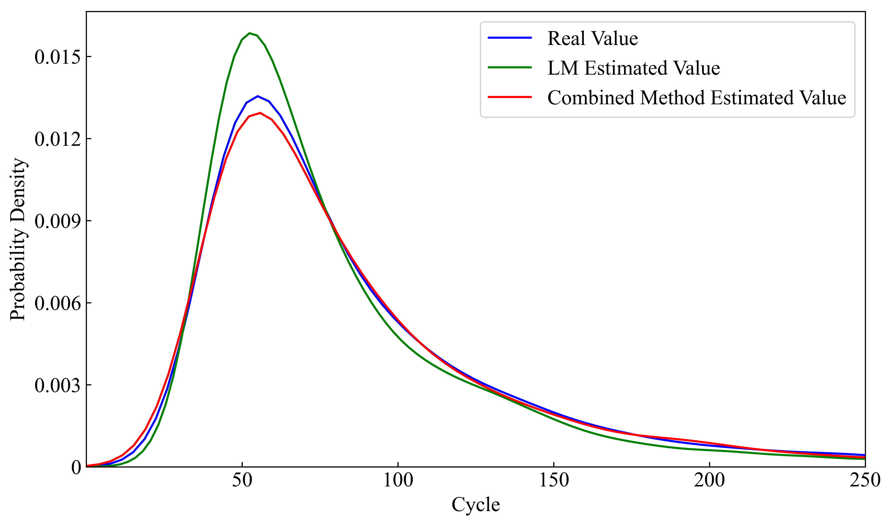
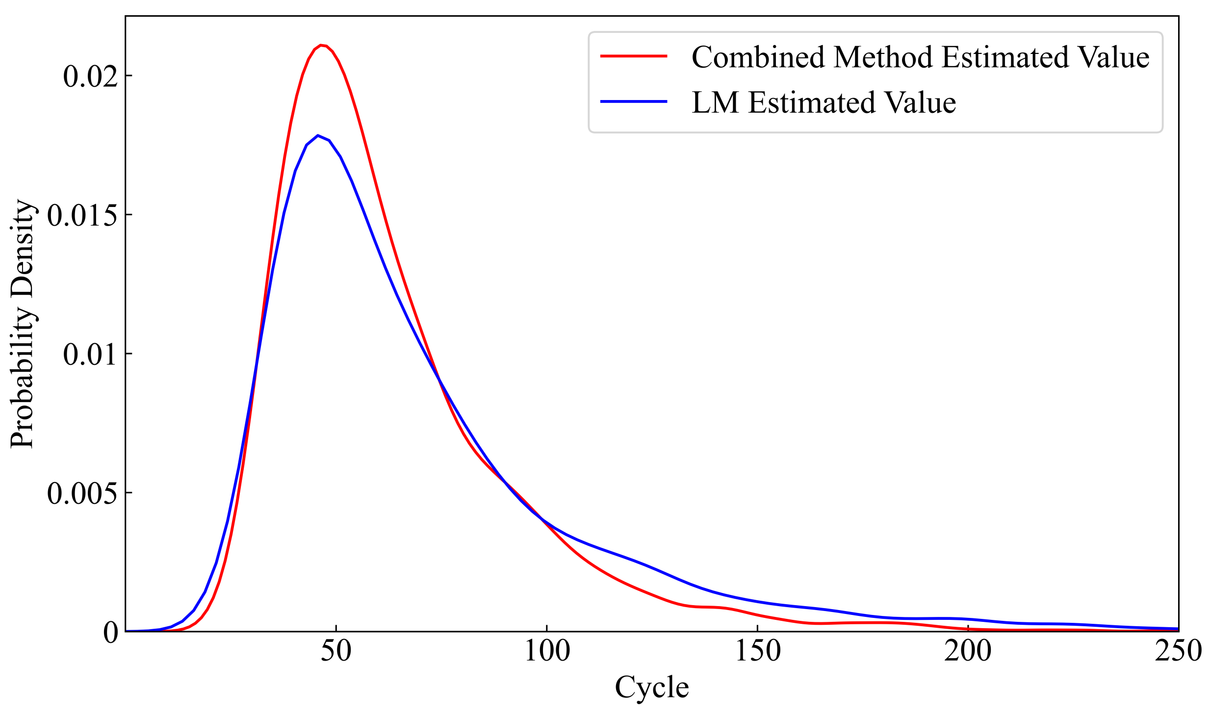
With the parameter estimates ${\widehat{\theta }}_{\mathrm{LM}}$ and $\widehat{\theta }$, the probability density functions of the failure time $T_D$ are also estimated and plotted in Figure 4. We regard a Li-ion battery to be failed once there is a $20\%$ fade in capacity, so the threshold used to define the failure time $T_D$ is set as $D=2.0353\times 80\%=1.6282$, where $2.0353$ Ahr is the original capacity of the battery $\#6$. As shown in Figure 4, the estimated PDF obtained by the combined method (red line) is thinner and taller than the one by the LM method (blue line). This implies that without the MCMC method, the density function will be estimated with heavier tails. This heavy-tail characteristic is also observed in

Table 9. Some characteristics of the density functions of $T_D$: $D=1.6282$.

	Mean	Mode	Median	5% Percentile	95% Percentile
Wiener	58	22	43	12	156
Wiener + error	57	41	52	24	110
LM method	71	44	58	33	149
Combined method	63	51	56	33	120

, when the $5\%$ and $95\%$ percentiles are compared. Although the $5\%$ percentiles are the same for the two methods, the $95\%$ percentile for the combined method is clearly less than that for the LM method.

Table 9 also reports some other characteristic values of the failure time $T_D$ and makes a comparison to the Wiener process model and the degradation model proposed by [21]. In [21], a logistic distributed measurement error is introduced to the basic Wiener process. From the values in Table 9, we see great differences among the characteristic values for the considered models, and this diversity may introduce troubles to further decision-making for battery health management. However, it is worth noting that with the threshold of $1.6282$, the real failure time for the battery $\#6$ is 61 cycles, which can be easily obtained from the data set. This failure time is best estimated by the mean of the estimated PDF given by the jump-diffusion model with the combined estimation method, which is 63 cycles. This relatively better performance in predicting failure time may be contributed to the inclusion of the jump process in the degradation model, which deems the capacity regeneration a part of the internal mechanism in battery aging. On the contrary, the basic Wiener process and the model in [21] attempt to filter out the effect of capacity regeneration on prediction by treating it originated from external interference. Moreover, these different modeling ways may explain why most characteristics in Table 9, except the $95\%$ percentile, always have larger values for the jump-diffusion model, no matter which of the two estimation methods is used.

Therefore, it may be suggested to use the estimation results obtained by the jump-diffusion model with the combined estimation method to make decisions. For example, the $5\%$ percentile for the model tells us that with properties and testing conditions similar to the battery $\#6$, about $5\%$ of the batteries would survive less than 33 cycles. This information would be helpful in the warranty design for the cycle-life of batteries. Moreover, conservative maintenance can be planned by considering replacing in-use batteries when they have worked for 51 cycles, which is the median of the estimated density.

6. Conclusions

This paper aims to model the degradation process of Li-ion batteries, which manifests itself in a loss in capacity. However, the capacity data set shows that the capacity regeneration phenomenon would appear due to a long relaxation period. To simultaneously describe the capacity loss and regeneration, a jump-diffusion model was considered, with the diffusion part represented by a geometric Brownian process and the jump part modeled by a compound homogeneous Poisson process. When estimating model parameters, the LM jump-detection test was adopted to identify the jump arrival times and separate battery degradation data to two series, jump series and diffusion series. Based on the two series of data, an initial estimation for the model parameters was given. Furthermore, with the help of probabilistic programming, the MCMC sampling algorithm was utilized to obtain final parameter estimates. Besides, the prediction of the failure time and RUL were also discussed. Simulation results suggested that the jump-diffusion model and the estimation method are feasible in modeling the battery capacity data and predicting the RUL. The good performance of the model was also demonstrated by the real data analysis.

Although it is the geometric Brownian process taken as the basic diffusion model in this paper, other Winer-process-based models are also good candidates as long as they satisfy the conditions required by the LM jump detection test. Similarly, rather than Poisson-type jumps, other suitably pure jump models also can be considered for describing the capacity regeneration phenomenon. But for any of the possible jump-diffusion models, the parameter estimation would still be a difficult task since the complication of the associated likelihood function. Therefore, future research should focus more on the estimation problems for both the model parameters and the RUL. Moreover, if the estimation is carried out in the Bayesian framework, it would be interesting and crucial to study how to make a good choice on priors, which are known to have great influences on estimation accuracy.

In this paper, only the capacity data itself was adopted to model the degradation evolution of Li-ion battery. In fact, batteries are usually used in time-varying environments, and their life can be affected by many dynamic external variables, such as charging current, charging voltage, charging power, temperature, etc. Hence, it is necessary and interesting to incorporate the external information into degradation models so that batteries’ reliability can be predicted more accurately. By treating the external variables as time-varying covariates, the model considered in this paper can be extended. For the parameter estimation, the LM detection test still can be used to identify the times at which the capacity regeneration occurs, and the Bayesian framework together with the MCMC algorithm is also a feasible method.