An Exact and Near-Exact Distribution Approach to the Behrens–Fisher Problem

Abstract

The Behrens–Fisher problem occurs when testing the equality of means of two normal distributions without the assumption that the two variances are equal. This paper presents approaches based on the exact and near-exact distributions for the test statistic of the Behrens–Fisher problem, depending on different combinations of even or odd sample sizes. We present the exact distribution when both sample sizes are odd and the near-exact distribution when one or both sample sizes are even. The near-exact distributions are based on a finite mixture of generalized integer gamma (GIG) distributions, used as an approximation to the exact distribution, which consists of an infinite series. The proposed tests, based on the exact and the near-exact distributions, are compared with Welch’s t-test through Monte Carlo simulations, in particular for small and unbalanced sample sizes. The results show that the proposed approaches are competent solutions to the Behrens–Fisher problem, exhibiting precise sizes and better powers than Welch’s approach for those cases. Numerical studies show that the Welch’s t-test tends to be a bit more conservative than the test statistics based on the exact or near-exact distribution, in particular when sample sizes are small and unbalanced, situations in which the proposed exact or near-exact distributions obtain higher powers than Welch’s t-test.

1. Introduction

Let us suppose we have two independent random samples $X_{1i},i=1,\dots ,n_1$ and $X_{2i},i=1,\dots ,n_2$, which are drawn from two normal distributions, $N\left({\mu }_1,{\sigma }_1^2\right)$ and $N\left({\mu }_2,{\sigma }_2^2\right)$, respectively. The Behrens–Fisher problem occurs when testing the equality of the two means ${\mu }_1$ and ${\mu }_2$ based on random samples like these without the assumption that the two variances, ${\sigma }_1^2$ and ${\sigma }_2^2$, are equal. [1] showed that a uniformly most powerful test does not exist in this case, and the Behrens–Fisher problem remains one of the unsolved problems of statistics. Many different approaches have been tried to solve this problem. Among those approaches are the fiducial approach proposed by [2,3], which somehow opened the way to the Bayesian approach proposed by [4,5], based on setting independent and locally uniform prior distributions for ${\mu }_1,{\mu }_2,log{\sigma }_1,log{\sigma }_2$. The frequentist approach proposed by [6,7] uses Student’s t distribution with ${\left(\frac{S_1^2}{n_1}+\frac{S_2^2}{n_2}\right)}^2/\left(\frac{S_1^4}{\left(n_1-1\right)n_1^2}+\frac{S_2^4}{\left(n_2-1\right)n_2^2}\right)$ degrees of freedom as the approximate distribution of the Behrens–Fisher statistic.

In this paper, we will obtain the exact and near-exact distributions, both the probability density function and cumulative distribution function, of the Behrens–Fisher statistic,

$$T^{*}=\frac{{\overline{X}}_1-{\overline{X}}_2}{\sqrt{\frac{S_1^2}{n_1}+\frac{S_2^2}{n_2}}},$$

(1)

under $H_0:{\mu }_1={\mu }_2$, where ${\overline{X}}_j=\frac{1}{n_j}{\sum }_{i=0}^{n_j}{X}_{ji}$ and $S_j^2=\frac{1}{n_j-1}{\sum }_{i=0}^{n_j}{\left(X_{ji}-{\overline{X}}_j\right)}^2$ for $j=1,2$, in the form of mixtures of Student’s t distributions multiplied by constants. Particularly for the case when both sample sizes are odd, the exact distribution will be derived in a finite closed form without any unsolved integrals or infinite sums by using the GIG (generalized integer gamma) distribution in [8], which is the distribution of the sum of independent gamma variables with integer shape parameters and nonequal rate parameters. For the other cases, that is, when both sample sizes are even or one of them is even and the other one is odd, the near-exact distribution will be obtained by approximating the exact distribution using a finite mixture of GIG distributions to obtain a more manageable cumulative distribution function. Such exact and near-exact distributions include ${\sigma }_1^2$ and ${\sigma }_2^2$ as unknown parameters, which have to be estimated, based on the observed samples, being then the p-values obtained from these exact or near-exact distributions with estimated parameters. The results will be compared with Welch’s t-test, one of the most widely used solutions to the problem, through Monte-Carlo simulations for relatively small sample sizes. We will see that the tests based on the exact or near-exact distribution show some advantage in terms of being able to obtain higher power than Welch’s t-test, especially when sample sizes are small and unbalanced and variances are also unbalanced.

This paper is organized as follows: Section 2 presents the exact distribution when both sample sizes are odd; Section 3 provides the near-exact distribution when one sample size is even and the other one odd, and Section 4 presents the exact near-exact distribution of the test statistic when both sample sizes are even. Numerical studies are provided in Section 5 to compare the exact and the near-exact distribution approaches with Welch’s t-test, and concluding remarks are presented in Section 6.

2. The Exact Distribution of the Behrens–Fisher Statistic for Odd-Numbered Sample Sizes

In this section, we present the exact distribution of the Behrens–Fisher statistic in (1), when both $n_1$ and $n_2$ are odd. Since $\frac{S_j^2}{n_j}=\frac{{\sigma }_j^2}{n_j\left(n_j-1\right)}\frac{\left(n_j-1\right)s_j^2}{{\sigma }_j^2}$ where $\frac{\left(n_j-1\right)s_j^2}{{\sigma }_j^2}\sim {\chi }_{n_j-1}^2(j=1,2),W=\frac{S_1^2}{n_1}+\frac{S_2^2}{n_2}$ is the sum of two independent gamma variables, each of which follows the distributions $\mathsf{\Gamma }\left(\frac{n_1-1}{2},\frac{n_1\left(n_1-1\right)}{2{\sigma }_1^2}\right)$ and $\mathsf{\Gamma }\left(\frac{n_2-1}{2},\frac{n_2\left(n_2-1\right)}{2{\sigma }_2^2}\right)$, where $\mathsf{\Gamma }(\mathrm{r},\lambda )$ indicates a gamma distribution with shape parameter $\mathrm{r}$ and rate parameter $\lambda$.

Now, we can divide the problem into two cases: one is the case of $\frac{n_1\left(n_1-1\right)}{2{\sigma }_1^2}\ne \frac{n_2\left(n_2-1\right)}{2{\sigma }_2^2}$, and the other is the case $\frac{n_1\left(n_1-1\right)}{2{\sigma }_1^2}=\frac{n_2\left(n_2-1\right)}{2{\sigma }_2^2}$. When $\frac{n_1\left(n_1-1\right)}{2{\sigma }_1^2}\ne \frac{n_2\left(n_2-1\right)}{2{\sigma }_2^2},W$ follows a GIG distribution of depth 2 with shape parameters $r_j=\frac{n_j-1}{2}$$(j=1,2)$ and rate parameters ${\lambda }_j=\frac{n_j\left(n_j-1\right)}{2{\sigma }_j^2}$$(j=1,2)$, which are different. Notice that $\frac{n_1-1}{2}$ and $\frac{n_2-1}{2}$ are both integers because of odd-numbered sample sizes. The probability density function for this distribution is

$$f_W\left(w\right)=\sum _{j=1}^2\sum _{k=1}^{r_j}\left(\prod _{j=1}^2{\lambda }_j^{r_j}\right)c_{j,k}{w}^{k-1}{e}^{-{\lambda }_{j}w}I(w>0)$$

where $c_{j,k}$ are given by (11)–(13) in [8]. In this case,

$$c_{i,r_i}=\frac{1}{\left(r_i-1\right)!}\prod _{j=1,j\ne i}^2{\left({\lambda }_j-{\lambda }_i\right)}^{-r_j}$$

and

$$c_{i,r_i-k}=\frac{1}{k}\sum _{j=1}^k\frac{\left(r_i-k+j-1\right)!}{\left(r_i-k-1\right)!}\left(\sum _{s=1,s\ne i}^2{r}_s{\left({\lambda }_i-{\lambda }_s\right)}^{-j}\right)c_{i,r_i-k+j}$$

for $k=1,\dots ,r_i-1,i=1,2$.

As a matter of fact, this probability density function can be rewritten as

$$f_W\left(w\right)={\displaystyle \sum _{j=1}^2}\sum _{k=1}^{r_j}\underset{p_{j,k}}{\underbrace{\left(\prod _{j=1}^2{\lambda }_j{}^{r_j}\right)c_{j,k}\frac{\mathsf{\Gamma }\left(k\right)}{{\lambda }_j{}^k}}}\underset{\mathrm{probability} \mathrm{density} \mathrm{function} \mathrm{of} \mathsf{\Gamma }\left(k,{\lambda }_j\right)}{\underbrace{\frac{{\lambda }_j{}^k}{\mathsf{\Gamma }\left(k\right)}{w}^{k-1}{e}^{-{\lambda }_{j}w}}}I(w>0)$$

which is a finite mixture of integer gamma distributions in [9]. Now that we have obtained the exact distribution of W, we can easily get the joint distribution of W and $Y={\overline{X}}_1-{\overline{X}}_2$, under $H_0:{\mu }_1={\mu }_2$. Y follows a normal distribution $N\left(0,\frac{{\sigma }_1^2}{n_1}+\frac{{\sigma }_2^2}{n_2}\right)$ under $H_0$, and so, given the independence of W and Y, the joint probability density function of these two random variables is

$$f_{W,Y}(w,y)=\sum _{j=1}^2\sum _{k=1}^{r_j}{p}_{j,k}\frac{{\lambda }_j^k}{\mathsf{\Gamma }\left(k\right)}{w}^{k-1}{e}^{-{\lambda }_{j}w}\frac{1}{\sigma }\mathsf{\Phi }\left(\frac{y}{\sigma }\right)(w>0,y\in (-\infty ,\infty ))$$

where $\sigma =\sqrt{\frac{{\sigma }_1^2}{n_1}+\frac{{\sigma }_2^2}{n_2}}$ and $\mathsf{\Phi }$ is the probability density function of a standard normal distribution.

Since we want to derive the distribution of $T^{*}=\frac{Y}{\sqrt{W}}$, we need to go further and obtain the joint distribution of $T^{*}$ and $V=\sqrt{W}$ from $f_{W,Y}(w,y)$ by a simple change of variables. From this process, we obtain

$$\begin{array}{ccc}\hfill f_{T^{*},V}(t,v)& =& \sum _{j=1}^2\sum _{k=1}^{r_j}{p}_{j,k}\frac{2{\lambda }_j^k}{\mathsf{\Gamma }\left(k\right)}{v}^{2k}{e}^{-{\lambda }_j{v}^2}\frac{1}{\sigma }\mathsf{\Phi }\left(\frac{tv}{\sigma }\right),\hfill \end{array}$$

for $v>0$ and $t\in (-\infty ,\infty )$ and

$$\begin{array}{ccc}\hfill f_{T^{*}}\left(t\right)& =& \sum _{j=1}^2\sum _{k=1}^{r_j}{p}_{j,k}{\int }_0^{\infty }2\frac{{\lambda }_j^k}{\mathsf{\Gamma }\left(k\right)}{v}^{2k}{e}^{-{\lambda }_j{v}^2}\frac{1}{\sigma }\mathsf{\Phi }\left(\frac{tv}{\sigma }\right)dv,\hfill \end{array}$$

where

$${\int }_0^{\infty }2\frac{{\lambda }_j^k}{\mathsf{\Gamma }\left(k\right)}{v}^{2k}{e}^{-{\lambda }_j{v}^2}\frac{1}{\sigma }\mathsf{\Phi }\left(\frac{tv}{\sigma }\right)dv$$

yields the probability density function of a $\sigma \sqrt{\frac{{\lambda }_j}{k}}{T}_{2k}$ random variable, with $T_{2k}$ denoting a Student’s t distribution with $2k$ degrees of freedom.

Hence, $f_{T^{*}}\left(t\right)$ is a mixture of probability density functions of $\sigma \sqrt{\frac{{\lambda }_j}{k}}{T}_{2k}$ random variables $\left(k=1,\dots ,r_{j}j=1,2\right)$, with weights $p_{j,k}$. Given that the probability density function of Student’s t variable with n degrees of freedom is given by

$$f_{T_n}\left(t\right)=\frac{1}{B\left(\frac{n}{2},\frac{1}{2}\right)}\frac{1}{\sqrt{n}}{\left(1+\frac{t^2}{n}\right)}^{-(n+1)/2}$$

for $t\in (-\infty ,\infty )$, the probability density function of $T^{*}$, under $H_0$, can be rewritten as

$$\begin{array}{ccc}\hfill f_{T^{*}}\left(t\right)& =& \sum _{j=1}^2\sum _{k=1}^{r_j}{p}_{j,k}{\mathrm{f}}_{\sigma \sqrt{{\lambda }_j/k}{T}_{2k}}\left(t\right)\hfill \\ & =& \left(\prod _{j=1}^2{\lambda }_j^{r_j}\right)\frac{1}{\sigma \sqrt{2\pi }}\sum _{j=1}^2\sum _{k=1}^{r_j}{c}_{j,k}\mathsf{\Gamma }\left(k+\frac{1}{2}\right){\left(\frac{t^2}{2{\sigma }^2}+{\lambda }_j\right)}^{-\left(k+\frac{1}{2}\right)}\hfill \end{array}$$

for $t\in (-\infty ,\infty )$.

Then, the cumulative distribution function of $T^{*}$ would also be a mixture of cumulative distribution functions of $\sigma \sqrt{\frac{{\lambda }_j}{k}}{T}_{2k}\left(k=1,\dots ,r_{j}j=1,2\right)$ with weights $p_{j,k}$. For Student’s t distribution with even degrees of freedom, the cumulative distribution function is given by

$$\begin{array}{ccc}\hfill F_{T_{2k}}\left(t\right)& =& \frac{1}{2}+\frac{t}{B\left(k,\frac{1}{2}\right)}\frac{1}{\sqrt{2k}}{}_2{\mathrm{F}}_1\left(k+\frac{1}{2},\frac{1}{2};\frac{3}{2};-\frac{t^2}{2k}\right)\hfill \\ & =& \frac{1}{2}+\frac{t}{B\left(k,\frac{1}{2}\right)}\frac{1}{\sqrt{2k}}{}_2{\mathrm{F}}_1\left(1-k,1;\frac{3}{2};-\frac{t^2}{2k}\right)\hfill \\ & =& \frac{1}{2}+\frac{\mathsf{\Gamma }\left(k+\frac{1}{2}\right)}{\sqrt{2k}}\frac{t}{2}{\left(1+\frac{t^2}{2k}\right)}^{\frac{1}{2}-k}\sum _{i=0}^{k-1}\frac{{\left(\frac{t^2}{2k}\right)}^i}{\mathsf{\Gamma }\left(\frac{3}{2}+i\right)\mathsf{\Gamma }(k-i)}\hfill \end{array}$$

for $t\in (-\infty ,\infty )$, which is obtained by applying $\mathrm{15.3.3}$ and $\mathrm{15.4.1}$ from [10], where ${}_2{\mathrm{F}}_1$ denotes a Gaussian hypergeometric function.

Thus, the cumulative distribution function of $T^{*}$, under $H_0$, can be expressed as

$$\begin{array}{c}{\displaystyle F_{T^{*}}\left(t\right)=\sum _{j=1}^2\sum _{k=1}^{r_j}{p}_{j,k}{F}_{T_{2k}}\left(t/\sigma \sqrt{\frac{{\lambda }_j}{k}}\right)}\hfill \\ {\displaystyle =\frac{1}{2}+\sum _{j=1}^2\sum _{k=1}^{r_j}\frac{\left({\prod }_{j=1}^2{\lambda }_j^{r_j}\right)}{\sqrt{2{\sigma }^2}}{c}_{j,k}\frac{\mathsf{\Gamma }\left(k\right)\mathsf{\Gamma }\left(k+\frac{1}{2}\right)}{{\lambda }_j}\frac{t}{2}{\left(\frac{t^2}{2{\sigma }^2}+{\lambda }_j\right)}^{\frac{1}{2}-k}\sum _{i=0}^{k-1}\frac{{\left(\frac{t^2}{2{\sigma }^2{\lambda }_j}\right)}^i}{\mathsf{\Gamma }\left(\frac{3}{2}+i\right)\mathsf{\Gamma }(k-i)}}\hfill \end{array}$$

for $t\in (-\infty ,\infty )$.

The distribution of $T^{*}$ is much simpler when $\frac{n_1\left(n_1-1\right)}{2{\sigma }_1^2}=\frac{n_2\left(n_2-1\right)}{2{\sigma }_2^2}.$ Since the rate parameters of the two independent gamma variables, $\frac{S_1^2}{n_1}$ and $\frac{S_2^2}{n_2}$, are, in this case, equal, W simply follows the gamma distribution $\mathsf{\Gamma }\left(\frac{n_1+n_2-2}{2},\frac{n_1\left(n_1-1\right)}{2{\sigma }_1^2}=\frac{n_2\left(n_2-1\right)}{2{\sigma }_2^2}\right)$. Therefore, in this case, $T^{*}\equiv T_{n_1+n_2-2}$. This means that the probability density function and cumulative distribution function of $T^{*}$ are the same as those of Student’s $t$ distribution with $n_1+n_2-2$ degrees of freedom. The probability density function for this distribution is written as

$$f_{T^{*}}\left(t\right)=\frac{1}{B\left(\frac{n_1+n_2-2}{2},\frac{1}{2}\right)}\frac{1}{\sqrt{n_1+n_2-2}}{\left(1+\frac{t^2}{n_1+n_2-2}\right)}^{-\left(n_1+n_2-1\right)/2}$$

for $t\in (-\infty ,\infty )$.

Additionally, as $n_1+n_2-2$ is an even number when sample sizes are odd-numbered, the cumulative distribution function can be written as

$$F_{T^{*}}\left(t\right)=\frac{1}{2}+\frac{\mathsf{\Gamma }\left(\frac{n_1+n_2-1}{2}\right)}{\sqrt{n_1+n_2-2}}\frac{t}{2}{\left(1+\frac{t^2}{n_1+n_2-2}\right)}^{\frac{3-n_1-n_2}{2}}\sum _{i=0}^{\frac{n_1+n_2-4}{2}}\frac{{\left(\frac{t^2}{n_1+n_2-2}\right)}^i}{\mathsf{\Gamma }\left(\frac{3}{2}+i\right)\mathsf{\Gamma }\left(\frac{n_1+n_2-2}{2}-i\right)}$$

for $t\in (-\infty ,\infty )$.

3. The Exact and Near-Exact Distribution of the Behrens–Fisher Statistic for Even-Numbered Sample Sizes

In this section, we present the exact distribution of $T^{*}$ when sample sizes are both even. The exact distribution consists of an infinite series, but we provide a near-exact distribution based on a finite mixture of GIG distributions, which yields an approximation to the exact distribution.

3.1. The Exact Distribution

Unlike the case where both sample sizes are odd, $W=\frac{S_1^2}{n_1}+\frac{S_2^2}{n_2}$ does not follow a GIG distribution when both sample sizes are even. This is so because the shape parameters for $\mathsf{\Gamma }\left(\frac{n_1-1}{2},\frac{n_1\left(n_1-1\right)}{2{\sigma }_1^2}\right)$ and $\mathsf{\Gamma }\left(\frac{n_2-1}{2},\frac{n_2\left(n_2-1\right)}{2{\sigma }_2^2}\right)$ are not integers when sample sizes are even. However, we can use the Kummer confluent hypergeometric function to obtain the exact distribution of W for this case.

Given the integral definition of the Kummer confluent hypergeometric function, the probability density function of W, which is the sum of two independent gamma variables with shape parameters

$$r_j=\frac{n_j-1}{2},j=1,2,$$

(2)

and rate parameters

$${\lambda }_j=\frac{n_j\left(n_j-1\right)}{2{\sigma }_j^2},j=1,2,$$

(3)

can be expressed as

$$\begin{array}{ccc}\hfill f_W\left(w\right)& =& \frac{{\lambda }_1^{r_1}}{\mathsf{\Gamma }\left(r_1\right)}\frac{{\lambda }_2^{r_2}}{\mathsf{\Gamma }\left(r_2\right)}{e}^{-{\lambda }_{2}w}{\int }_0^w{e}^{\left({\lambda }_2-{\lambda }_1\right)s}{s}^{r_1-1}{(w-s)}^{r_2-1}ds\hfill \\ & =& \frac{{\lambda }_1^{r_1}{\lambda }_2^{r_2}}{\mathsf{\Gamma }\left(r_1+r_2\right)}{e}^{-{\lambda }_{2}w}{w}^{r_1+r_2-1}{}_1{F}_1\left(r_1,r_1+r_2,\left({\lambda }_2-{\lambda }_1\right)w\right)\hfill \end{array}$$

for $w>0$.

Since

$${}_1{F}_1\left(r_1,r_1+r_2,\left({\lambda }_2-{\lambda }_1\right)w\right)=\sum _{i=0}^{\infty }\frac{\mathsf{\Gamma }\left(r_1+i\right)}{\mathsf{\Gamma }\left(r_1\right)}\frac{\mathsf{\Gamma }\left(r_1+r_2\right)}{\mathsf{\Gamma }\left(r_1+r_2+i\right)}\frac{{\left({\lambda }_2-{\lambda }_1\right)}^i}{i!}{w}^i,$$

the probability density function of W can be further written as

$$\begin{array}{ccc}\hfill f_W\left(w\right)& =& \sum _{i=0}^{\infty }\frac{\mathsf{\Gamma }\left(r_1+i\right)}{\mathsf{\Gamma }\left(r_1\right)}\frac{{\lambda }_1^{r_1}{\lambda }_2^{r_2}}{\mathsf{\Gamma }\left(r_1+r_2+i\right)}\frac{{\left({\lambda }_2-{\lambda }_1\right)}^i}{i!}{w}^{r_1+r_2+i-1}{e}^{-{\lambda }_{2}w}\hfill \\ & =& \sum _{i=0}^{\infty }\underset{p_i}{\underbrace{\frac{\mathsf{\Gamma }\left(r_1+i\right)}{\mathsf{\Gamma }\left(r_1\right)i!}{\left(\frac{{\lambda }_1}{{\lambda }_2}\right)}^{r_1}{\left(1-\frac{{\lambda }_1}{{\lambda }_2}\right)}^i}}\underset{p.d.f \mathrm{of} \mathsf{\Gamma }\left(r_1+r_2+i,{\lambda }_2\right)}{\underbrace{\frac{{\lambda }_2^{r_1+r_2+i}}{\mathsf{\Gamma }\left(r_1+r_2+i\right)}{w}^{r_1+r_2+i-1}{e}^{-{\lambda }_{2}w}}},\hfill \end{array}$$

for $w>0$, which is the probability density function of an infinite mixture of gamma distributions with weights $p_i$$(i=0,1,\dots )$. Now, using a similar approach to the one used in Section 2 for the case of odd-numbered sample sizes, we can obtain the exact probability density function of $T^{*}$ under $H_0$ in the form of an infinite mixture of probability density functions of $\sigma \sqrt{\frac{{\lambda }_2}{r_1+r_2+i}}{T}_{2\left(r_1+r_2+i\right)}$ distributions, with weights $p_i$, for $i=0,1,\dots$. The probability density function of $T^{*}$ may be then stated as follows:

$$\begin{array}{ccc}\hfill f_{T^{*}}\left(t\right)& =& \sum _{i=0}^{\infty }{p}_i{f}_{\sigma \sqrt{\frac{{\lambda }_2}{r_1+r_2+i}}{T}_{2\left(r_1+r_2+i\right)}}\left(t\right)\hfill \\ & =& \sum _{i=0}^{\infty }{p}_i\frac{1}{B\left(r_1+r_2+i,\frac{1}{2}\right)\sqrt{2{\sigma }^2{\lambda }_2}}{\left(1+\frac{t^2}{2{\sigma }^2{\lambda }_2}\right)}^{-\left(r_1+r_2+i+\frac{1}{2}\right)}\hfill \end{array}$$

for $t\in (-\infty ,\infty )$.

Regarding the exact cumulative distribution function of $T^{*}$, under $H_0$, this cumulative distribution function would also be an infinite mixture of cumulative distribution functions of $\sigma \sqrt{\frac{{\lambda }_2}{r_1+r_2+i}}{T}_{2\left(r_1+r_2+i\right)}$ distributions, with weights $p_i$, for $i=0,1,\dots$. It can be written as

$$\begin{array}{ccc}& & F_{T^{*}}\left(t\right)\hfill \\ & =& \sum _{i=0}^{\infty }{p}_i{F}_{T_{2\left(r_1+r_2+i\right)}}\left(t/\sigma \sqrt{\frac{{\lambda }_2}{r_1+r_2+i}}\right)\hfill \\ & =& \frac{1}{2}+\sum _{i=0}^{\infty }{p}_i\frac{\mathsf{\Gamma }\left(r_1+r_2+i+\frac{1}{2}\right)}{\sqrt{2{\sigma }^2{\lambda }_2}}\frac{t}{2}{\left(1+\frac{t^2}{2{\sigma }^2{\lambda }_2}\right)}^{\frac{1}{2}-r_i}\sum _{k=0}^{r_i-1}\frac{{\left(\frac{t^2}{2{\sigma }^2{\lambda }_2}\right)}^k}{\mathsf{\Gamma }\left(\frac{3}{2}+k\right)\mathsf{\Gamma }\left(r_1+r_2+i-k\right)}\hfill \end{array}$$

(4)

for $t\in (-\infty ,\infty )$, where $r_i=r_1+r_2+i$, $p_i=\frac{\mathsf{\Gamma }\left(r_1+i\right)}{\mathsf{\Gamma }\left(r_1\right)i!}{\left(\frac{{\lambda }_1}{{\lambda }_2}\right)}^{r_1}{\left(1-\frac{{\lambda }_1}{{\lambda }_2}\right)}^i$, by applying the expression for $F_{T_{2k}}\left(t\right)$ obtained in Section 2.

As the exact cumulative distribution function of $T^{*}$ is expressed as an infinite sum when ${\lambda }_1\ne {\lambda }_2$, it is not much of a manageable cumulative distribution function. In order to obtain numerical values of this cumulative distribution function in a reasonable amount of time, use of an integer upper bound for the summation in i is required. However, the number of terms required in order to obtain a small enough truncation error is often very large. Hence, a near-exact distribution of $T^{*}$ with a manageable cumulative distribution function needs to be obtained for the case where ${\lambda }_1\ne {\lambda }_2$ so that quantiles and p-values can be computed in a faster and more practical way.

3.2. Near-Exact Distribution

In order to obtain a near-exact distribution for $T^{*}$, based on a finite mixture, we will first obtain a near-exact distribution for W and then derive the distribution of $T^{*}$ from this distribution of W.

Let $r_j^{*}=\frac{n_j-2}{2}$$(j=1,2)$, and let ${\lambda }_1\ne {\lambda }_2$. Then, the exact characteristic function of W is given by

$$\begin{array}{ccc}\hfill {\mathsf{\Phi }}_W\left(t\right)& =& {\lambda }_1^{r_1}{\left({\lambda }_1-\mathbf{i}t\right)}^{-r_1}{\lambda }_2^{r_2}{\left({\lambda }_2-\mathbf{i}t\right)}^{-r_2}\hfill \\ & =& {\lambda }_1^{r_1^{*}}{\left({\lambda }_1-\mathbf{i}t\right)}^{-r_1^{*}}{\lambda }_2^{r_2^{*}}{\left({\lambda }_2-\mathbf{i}t\right)}^{-r_2^{*}}{\lambda }_1^{0.5}{\left({\lambda }_1-\mathbf{i}t\right)}^{-0.5}{\lambda }_2^{0.5}{\left({\lambda }_2-\mathbf{i}t\right)}^{-0.5}\hfill \end{array}$$

where $\mathbf{i}$ is the imaginary number with ${\mathbf{i}}^2=-1$. Since ${\lambda }_1{}^{0.5}{\left({\lambda }_1-\mathbf{i}t\right)}^{-0.5}{\lambda }_2{}^{0.5}{\left({\lambda }_2-\mathbf{i}t\right)}^{-0.5}$ is the characteristic function of the sum of two independent gamma variables $\mathsf{\Gamma }\left(0.5,{\lambda }_1\right)$ and $\mathsf{\Gamma }\left(0.5,{\lambda }_2\right)$, we can make use of the probability density function of W expressed as an infinite mixture of probability density functions of gamma distributions obtained in Section 3.1 to write

$${\lambda }_1^{0.5}{\left({\lambda }_1-\mathbf{i}t\right)}^{-0.5}{\lambda }_2^{0.5}{\left({\lambda }_2-\mathbf{i}t\right)}^{-0.5}=\sum _{j=0}^{\infty }{p}_j{\lambda }_2^{j+1}{\left({\lambda }_2-\mathbf{i}t\right)}^{-(j+1)},$$

where $p_j=\frac{\mathsf{\Gamma }(0.5+j)}{\mathsf{\Gamma }\left(0.5\right)j!}{\left(\frac{{\lambda }_1}{{\lambda }_2}\right)}^{0.5}{\left(1-\frac{{\lambda }_1}{{\lambda }_2}\right)}^j$. This leads to

$${\mathsf{\Phi }}_W\left(t\right)={\lambda }_1^{r_1^{*}}{\left({\lambda }_1-\mathbf{i}t\right)}^{-r_1^{*}}{\lambda }_2^{r_2^{*}}{\left({\lambda }_2-\mathbf{i}t\right)}^{-r_2^{*}}\sum _{j=0}^{\infty }{p}_j{\lambda }_2^{j+1}{\left({\lambda }_2-\mathbf{i}t\right)}^{-(j+1)}.$$

Now, for a given integer $m^{*}$, we propose to approximate ${\mathsf{\Phi }}_W\left(t\right)$ by

$$\begin{array}{cc}\hfill {\mathsf{\Phi }}_W^{*}\left(t\right)& ={\lambda }_1{}^{r_1^{*}}{\left({\lambda }_1-\mathbf{i}t\right)}^{-r_1^{*}}{\lambda }_2{}^{r_2^{*}}{\left({\lambda }_2-\mathbf{i}t\right)}^{-r_2^{*}}\sum _{j=0}^{m^{*}}{\pi }_j{\lambda }_2{}^{j+1}{\left({\lambda }_2-\mathbf{i}t\right)}^{-(j+1)}\hfill \\ & =\sum _{j=0}^{m^{*}}{\pi }_j{\lambda }_1{}^{r_1^{*}}{\left({\lambda }_1-\mathbf{i}t\right)}^{-r_1^{*}}{\lambda }_2{}^{r_2^{*}+j+1}{\left({\lambda }_2-\mathbf{i}t\right)}^{-\left(r_2^{*}+j+1\right)}\hfill \end{array}$$

where ${\pi }_j\left(j=0,\dots ,m^{*}-1\right)$ are determined in such a way that satisfies

$${\left.\frac{{\partial }^h}{\partial t^h}{\mathsf{\Phi }}_W\left(t\right)\right|}_{t=0}={\left.\frac{{\partial }^h}{\partial t^h}{\mathsf{\Phi }}_W^{*}\left(t\right)\right|}_{t=0}\mathrm{for}h=1,\dots ,m^{*},$$

with ${\pi }_{m^{*}}=1-{\sum }_{i=0}^{m^{*}-1}{\pi }_i$. This approximate characteristic function ${\mathsf{\Phi }}_W^{*}\left(t\right)$ is, in fact, the characteristic function of a finite mixture (with weights ${\pi }_j$) of $m^{*}+1$ GIG distributions of depth 2 with integer shape parameters $r_1^{*},r_2^{*}+j+1$$\left(j=0,\dots ,m^{*}\right)$ and rate parameters ${\lambda }_1$ and ${\lambda }_2$, the first $m^{*}$ moments of which are the same as those of W.

Hence, a finite mixture of probability density functions of $m^{*}+1$ GIG distributions with weights ${\pi }_j$ for $j=0,\dots ,m^{*}$ will then be a near-exact probability density function of W. As the GIG distribution itself is a finite mixture of gamma distributions, as shown in Section 2, this probability density function can be written as

$$\begin{array}{ccc}\hfill f_W^{*}\left(w\right)& =& \sum _{i=0}^{m^{*}}{\pi }_i\sum _{j=1}^2\sum _{k=1}^{r_{ji}^{**}}\left(\prod _{j=1}^2{\lambda }_j^{r_{ji}^{**}}\right)c_{jk,i}^{*}{w}^{k-1}{e}^{-{\lambda }_{j}w}\hfill \\ & =& \sum _{i=0}^{m^{*}}{\pi }_i\sum _{j=1}^2\sum _{k=1}^{r_{ji}^{**}}\underset{p_{jk,i}^{*}}{\underbrace{\left(\prod _{j=1}^2{\lambda }_j^{r_{ji}^{**}}\right)c^{*}{}_{jk,i}\frac{\mathsf{\Gamma }\left(k\right)}{{\lambda }_j{}^k}}}\underset{\mathrm{p}.\mathrm{d}.\mathrm{f}\mathrm{of}\mathsf{\Gamma }\left(k,{\lambda }_j\right)}{\underbrace{\frac{{\lambda }_j{}^k}{\mathsf{\Gamma }\left(k\right)}{w}^{k-1}{e}^{-{\lambda }_{j}w}}}\hfill \end{array}$$

for $w>0$, where

$$r_{ji}^{**}=\left\{\begin{array}{cc}{r}_1^{*}\hfill & j=1\hfill \\ r_2^{*}+i+1\hfill & j=2\hfill \end{array}\right.$$

for $i=0,\dots ,m^{*}$ and $c_{jk,i}^{*}$ are defined in the same way as $c_{j,k}$ in Section 2, except here we use $r_{ji}^{**}$ instead of $r_j$.

From this near-exact probability density function of W, using the same logic as before just like in Section 2 and Section 3.1, we can obtain a near-exact probability density function of $T^{*}$ in the form of a finite mixture of probability density function $\mathrm{s}$ of $\sigma \sqrt{\frac{{\lambda }_j}{k}}{T}_{2k}$ with weights ${\pi }_i{p}_{jk,i}^{*}$. Thus, the near-exact probability density function under $H_0$ is given as follows:

$$\begin{array}{ccc}\hfill f_{T^{*}}^{*}\left(t\right)& =& \sum _{i=0}^{m^{*}}\sum _{j=1}^2\sum _{k=1}^{r_{ji}^{**}}{\pi }_i{p}_{jk,i}^{*}{f}_{\sigma \sqrt{\frac{{\lambda }_j}{k}}{T}_{2k}}\left(t\right)\hfill \\ & =& \sum _{i=0}^{m^{*}}\sum _{j=1}^2\sum _{k=1}^{r_{ji}^{**}}{\pi }_i\left(\prod _{j=1}^2{\lambda }_j^{r_{ji}^{**}}\right)c_{jk,i}^{*}\frac{\mathsf{\Gamma }(k+0.5)}{\sqrt{2\pi {\sigma }^2}}{\left({\lambda }_j+\frac{t^2}{2{\sigma }^2}\right)}^{-(k+0.5)}\hfill \end{array}$$

for $t\in (-\infty ,\infty )$. Naturally, the corresponding near-exact cumulative distribution function of $T^{*}$ would be a finite mixture of cumulative distribution function $\mathrm{s}$ of $\sigma \sqrt{\frac{{\lambda }_j}{k}}{T}_{2k}$ with weights ${\pi }_i{p}_{jk,i}^{*}$, which can be written as

$$\begin{array}{c}\hfill \begin{array}{ccc}{F}_{T^{*}}^{*}\left(t\right)& =& \frac{1}{2}+\sum _{i=0}^{m^{*}}\sum _{j=1}^2\sum _{k=1}^{r_{ji}^{**}}\{{\pi }_i\left(\prod _{j=1}^2{\lambda }_j{}_{ji}^{**}\right)c_{jk,i}^{*}\frac{\mathsf{\Gamma }\left(k\right)\mathsf{\Gamma }(k+0.5)}{\sqrt{2{\sigma }^2}}\frac{t}{2{\lambda }_j}{\left({\lambda }_j+\frac{{\mathrm{t}}^2}{2{\sigma }^2}\right)}^{0.5-\mathrm{k}}\\ & & \times \sum _{\mathrm{s}=0}^{\mathrm{k}-1}\frac{{\left(\frac{t^2}{2{\sigma }^2{\lambda }_j}\right)}^{\mathrm{s}}}{\mathsf{\Gamma }\left(\frac{3}{2}+s\right)\mathsf{\Gamma }(k-s)}\}\end{array}\end{array}$$

(5)

for $t\in (-\infty ,\infty )$, by applying $F_{T_{2k}}\left(t\right)$ obtained in Section 2.

4. One of the Sample Sizes Is Even and the Other Is Odd

The exact distribution of the Behrens–Fisher statistic $T^{*}$ for this case is given by the same expressions used in Section 3.1. Just like the case of even-numbered sample sizes, the exact cumulative distribution function is not that manageable for usage when ${\lambda }_1\ne {\lambda }_2$ in this case, too. Hence there is a need to obtain a near-exact distribution of $T^{*}$ with a manageable cumulative distribution function for faster and more practical computation of quantiles and $p$-values.

As we did in Section 3.2, we will first obtain a near-exact distribution for W, and then we will derive the near-exact distribution for $T^{*}$ from the distribution of W. Let, without any loss of generality, $n_1$ be even and $n_2$ be odd. Additionally, let $r_1^{*}=\frac{n_1-2}{2}$, which is equivalent to $\left[r_1\right]$, and let ${\lambda }_1\ne {\lambda }_2$. Then, for $r_j$ and ${\lambda }_j$ as defined in (2) and (3), the exact characteristic function of W can be written as

$$\begin{array}{ccc}\hfill {\mathsf{\Phi }}_W\left(t\right)& =& {\lambda }_1^{r_1}{\left({\lambda }_1-\mathbf{i}t\right)}^{-r_1}{\lambda }_2^{r_2}{\left({\lambda }_2-\mathbf{i}t\right)}^{-r_2}\hfill \\ & =& \underset{{\mathsf{\Phi }}_{W_1}\left(t\right)}{\underbrace{{\lambda }_1^{r_1^{*}}{\left({\lambda }_1-\mathbf{i}t\right)}^{-r_1^{*}}{{\lambda }_2}^{r_2}{\left({\lambda }_2-\mathbf{i}t\right)}^{-r_2}}}\underset{{\mathsf{\Phi }}_{W_2}\left(t\right)}{\underbrace{{\lambda }_1^{\frac{1}{2}}{\left({\lambda }_1-\mathbf{i}t\right)}^{-\frac{1}{2}}}},\hfill \end{array}$$

where ${\mathsf{\Phi }}_{W_1}\left(t\right)$ is the characteristic function of a GIG distribution of depth 2 with integer shape parameters $r_1^{*}$ and $r_2$ and rate parameters ${\lambda }_1$ and ${\lambda }_2$, while ${\mathsf{\Phi }}_{W_2}\left(t\right)$ is the characteristic function of a $\mathsf{\Gamma }\left(0.5,{\lambda }_1\right)$ distribution. Now, for a given $m^{*}\in \mathbb{N}$, we propose to approximate ${\mathsf{\Phi }}_{W_2}\left(t\right)$ by

$${\mathsf{\Phi }}_{W_2}^{*}\left(t\right)=\sum _{j=0}^{m^{*}}{\pi }_j{\left(2{\lambda }_1\right)}^{(j+1)}{\left(2{\lambda }_1-\mathbf{i}t\right)}^{-(j+1)}$$

where ${\pi }_j\left(j=0,\dots ,m^{*}-1\right)$ are determined in such a way that

$${\left.\frac{{\partial }^h}{\partial t^h}{\mathsf{\Phi }}_{W_2}\left(t\right)\right|}_{t=0}={\left.\frac{{\partial }^h}{\partial t^h}{\mathsf{\Phi }}_{W_2}^{*}\left(t\right)\right|}_{t=0}\mathrm{for}h=1,\dots ,m^{*}$$

with ${\pi }_{m^{*}}=1-{\sum }_{i=0}^{m^{*}-1}{\pi }_i$.

The characteristic function ${\mathsf{\Phi }}_{W_2}^{*}\left(t\right)$ is the characteristic function of a finite mixture of $m^{*}+1$ distributions, which are $\mathsf{\Gamma }\left(j+1,2{\lambda }_1\right)$ distributions $\left(j=0,\dots ,m^{*}\right)$. The first $m^{*}$ moments of this mixture are the same as those of $\mathsf{\Gamma }\left(0.5,{\lambda }_1\right)$.

We should note that the weights ${\pi }_j$ do not depend on ${\lambda }_1$. The h-th non-central moment of $\mathsf{\Gamma }\left(0.5,{\lambda }_1\right)$ and of the mixture of $\mathsf{\Gamma }\left(j+1,2{\lambda }_1\right)$ distributions are, respectively, given by

$$\frac{\mathsf{\Gamma }\left(h+\frac{1}{2}\right)}{\mathsf{\Gamma }\left(\frac{1}{2}\right){\lambda }_1{}^h}\mathrm{and}\sum _{j=0}^{m^{*}}{\pi }_j\frac{\mathsf{\Gamma }(h+j+1)}{\mathsf{\Gamma }(j+1){\left(2{\lambda }_1\right)}^h},$$

which means ${\pi }_j$ are determined in such a way that satisfies

$$\frac{\mathsf{\Gamma }\left(h+\frac{1}{2}\right)}{\mathsf{\Gamma }\left(\frac{1}{2}\right)}=\sum _{j=0}^{m^{*}}{\pi }_j\frac{\mathsf{\Gamma }(h+j+1)}{\mathsf{\Gamma }(j+1)2^h},$$

for $h=1,\dots ,m^{*}$, definitely not depending on ${\lambda }_1$.

By using ${\mathsf{\Phi }}_{W_2}^{*}\left(t\right)$ instead of ${\mathsf{\Phi }}_{W_2}\left(t\right)$, we can then approximate ${\mathsf{\Phi }}_W\left(t\right)$ with

$$\begin{array}{cc}\hfill {\mathsf{\Phi }}_W^{*}\left(t\right)& ={\lambda }_1^{r_1^{*}}{\left({\lambda }_1-\mathbf{i}t\right)}^{-r_1^{*}}{\lambda }_2^{r_2}{\left({\lambda }_2-\mathbf{i}t\right)}^{-r_2}\sum _{j=0}^{m^{*}}{\pi }_j{\left(2{\lambda }_1\right)}^{(j+1)}{\left(2{\lambda }_1-\mathbf{i}t\right)}^{-(j+1)}\hfill \\ \hfill =& \sum _{j=0}^{m^{*}}{\pi }_j{\lambda }_1^{r_1^{*}}{\left({\lambda }_1-\mathbf{i}t\right)}^{-r_1^{*}}{\lambda }_2^{r_2}{\left({\lambda }_2-\mathbf{i}t\right)}^{-r_2}{\left(2{\lambda }_1\right)}^{(j+1)}{\left(2{\lambda }_1-\mathbf{i}t\right)}^{-(j+1)}\hfill \end{array}$$

which is the characteristic function of a finite mixture of $m^{*}+1\mathrm{GIG}$ distributions of depth 3 with shape parameters $r_1^{*},r_2,j+1\left(j=0,\dots ,m^{*}\right)$ and rate parameters ${\lambda }_1,{\lambda }_2,2{\lambda }_1$.

Thus, a finite mixture of $m^{*}+1$ probability density functions s of $GIG$ distributions of depth 3 with weights ${\pi }_j$ can be a near-exact probability density function of W. As GIG distribution itself is a finite mixture of gamma distributions, this near-exact probability density function of W is written as

$$\begin{array}{ccc}\hfill {\displaystyle f_W^{*}\left(w\right)}& =& {\displaystyle \sum _{i=0}^{m^{*}}{\pi }_i\sum _{j=1}^3\sum _{k=1}^{r_{ji}^{*}}\left(\prod _{j=1}^3{\left({\lambda }_j^{*}\right)}^{r_{ji}^{*}}\right)c_{jk,i}^{*}{w}^{k-1}{e}^{-{\lambda }_j^{*}w}}\hfill \\ & =& {\displaystyle \sum _{i=0}^{m^{*}}{\pi }_i\sum _{j=1}^3\sum _{k=1}^{r_{ji}^{*}}\underset{p_{jk,i}^{*}}{\underbrace{\left(\prod _{j=1}^3{\left({\lambda }_j^{*}\right)}^{r_{ji}^{*}}\right)c_{jk,i}^{*}\frac{\mathsf{\Gamma }\left(k\right)}{{\left({\lambda }_j^{*}\right)}^k}}}\underset{\mathrm{p}.\mathrm{d}.\mathrm{f}\mathrm{of}\mathsf{\Gamma }\left(k,{\lambda }_j^{*}\right)}{\underbrace{\frac{{\left({\lambda }_j^{*}\right)}^k}{\mathsf{\Gamma }\left(k\right)}{w}^{k-1}{e}^{-{\lambda }^{*}w}}}(w>0)}\hfill \end{array}$$

where

$$r_{ji}^{*}=\left\{\begin{array}{cc}{r}_1^{*}\hfill & j=1\hfill \\ r_2\hfill & j=2\hfill \\ i+1\hfill & j=3\hfill \end{array}\left(i=0,\dots ,m^{*}\right)\right.,{\lambda }_j^{*}=\left\{\begin{array}{cc}{\lambda }_1\hfill & j=1\hfill \\ {\lambda }_2\hfill & j=2\hfill \\ 2{\lambda }_1\hfill & j=3\hfill \end{array}\right.$$

and $c_{jk,i}^{*}$ are given by (11)–(13) in [8] using $r_{ji}^{*}$ and ${\lambda }_j^{*}$, which are

$$\begin{array}{cc}& c_{j,r_{ji}^{*},i}=\frac{1}{\left(r_{ji}^{*}-1\right)!}\prod _{\mathrm{s}=1,\mathrm{s}\ne j}^3{\left({\lambda }_{\mathrm{s}}^{*}-{\lambda }^{*}{}_j\right)}^{-r_{si}^{*}},\hfill \\ & c_{j,r_{ji}^{*}-k,i}^{*}=\frac{1}{k}\sum _{\mathrm{n}=1}^k\frac{\left(r_{ji}^{*}-k+n-1\right)!}{\left(r_{ji}^{*}-k-1\right)!}\left(\sum _{s=1,\mathrm{s}\ne j}^3{r}_s{\left({\lambda }_j^{*}-{\lambda }_{\mathrm{s}}^{*}\right)}^{-n}\right)c_{j,r_{ji}^{*}-k+n,i}\hfill \end{array}$$

where $k=1,\dots ,r_{ji}^{*}-1$ and $j=1,2,3,i=0,\dots ,m^{*}$. From this near-exact probability density function of W, using the same logic as before, we can once again obtain a near-exact probability density function of $T^{*}$ in the form of a finite mixture of probability density functions of $\sigma \sqrt{\frac{{\lambda }_j^{*}}{k}}{T}_{2k}$ distributions, with weights ${\pi }_i{p}_{jk,i}^{*}$. The near-exact probability density function of $T^{*}$, under $H_0$, is thus given by

$$\begin{array}{ccc}\hfill f_{T^{*}}^{*}\left(t\right)& =& \sum _{i=0}^{m^{*}}\sum _{j=1}^3\sum _{k=1}^{r_{ji}^{*}}{\pi }_i{p}_{jk,i}^{*}{f}_{\sigma \sqrt{\frac{{\lambda }_j^{*}}{k}}{T}_{2k}}\left(t\right)\hfill \\ & =& \sum _{i=0}^{m^{*}}\sum _{j=1}^3\sum _{k=1}^{r_{ji}^{*}}{\pi }_i\left(\prod _{j=1}^3{\left({\lambda }_j^{*}\right)}^{r_{ji}^{*}}\right)c_{jk,i}^{*}\frac{\mathsf{\Gamma }\left(k+\frac{1}{2}\right)}{\sqrt{2\pi {\sigma }^2}}{\left({\lambda }_j^{*}+\frac{t^2}{2{\sigma }^2}\right)}^{-\left(k+\frac{1}{2}\right)}\hfill \end{array}$$

for $t\in (-\infty ,\infty )$.

Hence, the corresponding near-exact cumulative distribution function of $T^{*}$, under $H_0$, is also a finite mixture of cumulative distribution functions of $\sigma \sqrt{\frac{{\lambda }_j^{*}}{k}}{T}_{2k}$, with weights ${\pi }_i{p}_{jk,i}^{*}$, which can be written as

$$\begin{array}{c}\hfill \begin{array}{ccc}{F}_{T^{*}}^{*}\left(t\right)& =& \frac{1}{2}+\sum _{i=0}^{m^{*}}\sum _{j=1}^3\sum _{k=1}^{r_{ji}^{*}}\{{\pi }_i\left(\prod _{j=1}^3{\left({\lambda }_j^{*}\right)}^{r_{ji}^{*}}\right)c_{jk,i}^{*}\frac{\mathsf{\Gamma }\left(k\right)\mathsf{\Gamma }(k+0.5)}{\sqrt{2{\sigma }^2}}\frac{t}{2{\lambda }_j^{*}}{\left({\lambda }_j^{*}+\frac{t^2}{2{\sigma }^2}\right)}^{0.5-k}\\ & & \times \sum _{\mathrm{s}=0}^{k-1}\frac{{\left(\frac{t^2}{2{\sigma }^2{\lambda }_j^{*}}\right)}^{\mathrm{s}}}{\mathsf{\Gamma }\left(\frac{3}{2}+s\right)\mathsf{\Gamma }(k-s)}\}\end{array}\end{array}$$

(6)

for $t\in (-\infty ,\infty )$ by applying $F_{T_{2k}}\left(t\right)$ obtained in Section 2.

5. Comparison of the Exact or Near-Exact Distribution and Welch’s t Test

When it is plausible to assume that ${\lambda }_1\ne {\lambda }_2$, that is, that $\frac{n_1\left(n_1-1\right)}{2{\sigma }_1^2}\ne \frac{n_2\left(n_2-1\right)}{2{\sigma }_2^2}$, we can make use of the exact and near-exact distribution of $T^{*}$ to solve the Behrens–Fisher problem. The exact cumulative distribution function of $T^{*}$ will be used for computation of p-values when both sample sizes are odd, while the near-exact cumulative distribution functions obtained in Section 3 and Section 4 will be used for computing p-values when both sample sizes are even or when one of the sample sizes is even and the other is odd. Because the cumulative distribution functions of $T^{*}$ include the unknown parameters ${\sigma }_1^2$ and ${\sigma }_2^2$, these will be estimated by the sample variances $S_i^2$$(i=1,2)$.

We will compare the exact or near-exact distributions and Welch’s t-test by their actual sizes and powers for testing $H_0:{\mu }_1={\mu }_2$ versus $H_1:{\mu }_1>{\mu }_2$. For $T^{*}=t$, since the hypothesis is for the right-tailed test, the corresponding p-value is computed from $1-F_{T^{*}}\left(t\right)$ in (4) or $1-F_{T^{*}}^{*}\left(t\right)$ in (5) or (6), depending on the parity of the sample sizes, according to the derivations in the previous sections, and with $\sigma$ estimated by $\widehat{\sigma }=\sqrt{S_1^2/n_1+S_2^2/n_2}$. We used different type I error rates $\alpha \in \{0.1,0.05,0.01\}$ and we conducted Monte Carlo experiments under a range of different sets of parameters.

Simulations were conducted for variance and sample size pairs that correspond to

$$\theta =\frac{{\sigma }_1^2}{n_1}/\left(\frac{{\sigma }_1^2}{n_1}+\frac{{\sigma }_2^2}{n_2}\right)\in \{0.1,0.3,0.5\}.$$

For ${\mu }_1-{\mu }_2$, we covered the cases where ${\mu }_1-{\mu }_2$ satisfies

$$\delta =\frac{{\mu }_1-{\mu }_2}{\sqrt{\frac{{\sigma }_1^2}{n_1}+\frac{{\sigma }_2^2}{n_2}}}\in \{0,1,2\},$$

with $\delta =0$ corresponding to the null hypothesis $H_0:{\mu }_1={\mu }_2$.

For each combination of parameters, the number of replications was 50,000, and in each subsection, we provide two scenarios: one in which sample sizes were balanced, and another one where they were unbalanced. For each generated sample, we computed $t_i$ for $i=1,\dots ,$ 50,000 and then obtained the type I error under $\delta =0$ and the power under $\delta >0$ from

$$\begin{array}{c}\hfill \frac{1}{50,000}\sum _{i=1}^{50,000}I(p_i\le \alpha )\end{array}$$

(7)

where $I(·)$ is the indicator function and the p-value $p_i=1-F_{T^{*}}\left(t_i\right)$ is computed using $F_{T^{*}}(·)$ in (4) for the case of both odd sample sizes or $F_{T^{*}}(·)$ in (5) or (6) when at least one of the sample sizes is even.

All computations were done with the software R, version 4.1.0.

5.1. Odd n₁ and n₂

In

Table 1. Power values for $\left(n_1,n_2\right)=(5,5)$.

$\mathsf{\theta }$	$\mathsf{\alpha }$	$\mathsf{\delta }=0$		$\mathsf{\delta }=1$		$\mathsf{\delta }=2$
		E	W	E	W	E	W
$0.1$	$0.1$	$0.1009$	$0.1000$	$0.3578$	$0.3558$	$0.7059$	$0.7036$
${\sigma }_1^2=5$	$0.05$	$0.0518$	$0.0506$	$0.2234$	$0.2199$	$0.5368$	$0.5313$
${\sigma }_2^2=45$	$0.01$	$0.0123$	$0.0114$	$0.0731$	$0.0676$	$0.2291$	$0.2139$
$0.3$	$0.1$	$0.0971$	$0.0965$	$0.3664$	$0.3648$	$0.7205$	$0.7187$
${\sigma }_1^2=15$	$0.05$	$0.0480$	$0.0473$	$0.2271$	$0.2241$	$0.5528$	$0.5482$
${\sigma }_2^2=35$	$0.01$	$0.0100$	$0.0092$	$0.0636$	$0.0601$	$0.2376$	$0.2263$
$0.5$	$0.1$	$0.0958$	$0.0953$	$0.3628$	$0.3614$	$0.7221$	$0.7205$
${\sigma }_1^2=5$	$0.05$	$0.0462$	$0.0456$	$0.2243$	$0.2218$	$0.5582$	$0.5545$
${\sigma }_2^2=5$	$0.01$	$0.0094$	$0.0005$	$0.0641$	$0.0606$	$0.2375$	$0.2288$

and

Table 2. Power values for $\left(n_1,n_2\right)=(15,3)$.

$\mathsf{\theta }$	$\mathsf{\alpha }$	$\mathsf{\delta }=0$		$\mathsf{\delta }=1$		$\mathsf{\delta }=2$
		E	W	E	W	E	W
$0.1$	$0.1$	$0.1100$	$0.1048$	$0.3542$	$0.3402$	$0.6614$	$0.6441$
${\sigma }_1^2=15$	$0.05$	$0.0660$	$0.0595$	$0.2304$	$0.2090$	$0.4893$	$0.4522$
${\sigma }_2^2=27$	$0.01$	$0.0273$	$0.0053$	$0.1076$	$0.0843$	$0.2609$	$0.1987$
$0.3$	$0.1$	$0.1052$	$0.1013$	$0.3636$	$0.3538$	$0.7033$	$0.6900$
${\sigma }_1^2=45$	$0.05$	$0.0593$	$0.0557$	$0.2434$	$0.2287$	$0.5414$	$0.5133$
${\sigma }_2^2=21$	$0.01$	$0.0180$	$0.0161$	$0.0990$	$0.0872$	$0.2940$	$0.2533$
$0.5$	$0.1$	$0.1001$	$0.0976$	$0.3743$	$0.3679$	$0.7263$	$0.7185$
${\sigma }_1^2=15$	$0.05$	$0.0532$	$0.0507$	$0.2390$	$0.2301$	$0.5657$	$0.5488$
${\sigma }_2^2=3$	$0.01$	$0.0133$	$0.0119$	$0.0866$	$0.0788$	$0.2949$	$0.2687$

, we present the power values for the exact distribution and Welch’s test, represented, respectively, by E and W. We considered for $\theta$ and $\delta$ the sets of values indicated above.

We may see that when sample sizes are unbalanced, as in Table 2, the exact distribution gives larger values of power than Welch’s t-test, namely for larger values of $\delta$ and smaller values of $\alpha$, while they tend to give similar results when the two sample sizes are homogeneous, still with the exact distribution giving larger power values when the variances are unbalanced. Namely, for the case of $(n_1,n_2)=(15,3)$ and $({\sigma }_1^2,{\sigma }_2^2)=(15,27)$ and $\delta =2$, the near-exact distribution shows a gain of over 30% in power in relation to Welch’s t-test for $\alpha =0.01$.

5.2. Even $n_1$ and $n_2$

Table 3. Power values for $\left(n_1,n_2\right)=(8,8)$.

$\mathsf{\theta }$	$\mathsf{\alpha }$	$\mathsf{\delta }=0$		$\mathsf{\delta }=1$		$\mathsf{\delta }=2$
		NE	W	NE	W	NE	W
$0.1$	$0.1$	$0.1002$	$0.0998$	$0.3731$	$0.3722$	$0.7319$	$0.7311$
${\sigma }_1^2=8$	$0.05$	$0.0525$	$0.0519$	$0.2384$	$0.2371$	$0.5775$	$0.5750$
${\sigma }_2^2=72$	$0.01$	$0.0111$	$0.0106$	$0.0755$	$0.0726$	$0.2747$	$0.2672$
$0.3$	$0.1$	$0.1001$	$0.0992$	$0.3746$	$0.3741$	$0.7392$	$0.7395$
${\sigma }_1^2=24$	$0.05$	$0.0497$	$0.0488$	$0.2373$	$0.2360$	$0.5927$	$0.5922$
${\sigma }_2^2=56$	$0.01$	$0.0105$	$0.0094$	$0.0760$	$0.0744$	$0.2929$	$0.2879$
$0.5$	$0.1$	$0.0981$	$0.0968$	$0.3775$	$0.3772$	$0.7370$	$0.7385$
${\sigma }_1^2=8$	$0.05$	$0.0511$	$0.0495$	$0.2403$	$0.2393$	$0.5942$	$0.5947$
${\sigma }_2^2=8$	$0.01$	$0.0103$	$0.0087$	$0.0757$	$0.0739$	$0.2911$	$0.2890$

and

Table 4. Power values for $\left(n_1,n_2\right)=(12,4)$.

$\mathsf{\theta }$	$\mathsf{\alpha }$	$\mathsf{\delta }=0$		$\mathsf{\delta }=1$		$\mathsf{\delta }=2$
		NE	W	NE	W	NE	W
$0.1$	$0.1$	$0.1061$	$0.1020$	$0.3554$	$0.3458$	$0.6925$	$0.6823$
${\sigma }_1^2=12$	$0.05$	$0.0578$	$0.0539$	$0.2293$	$0.2129$	$0.5233$	$0.4974$
${\sigma }_2^2=36$	$0.01$	$0.0175$	$0.0148$	$0.0894$	$0.0725$	$0.2568$	$0.2082$
$0.3$	$0.1$	$0.1031$	$0.1009$	$0.3666$	$0.3612$	$0.7186$	$0.7120$
${\sigma }_1^2=36$	$0.05$	$0.0545$	$0.0523$	$0.2361$	$0.2266$	$0.5657$	$0.5492$
${\sigma }_2^2=28$	$0.01$	$0.0131$	$0.0117$	$0.0864$	$0.0769$	$0.2781$	$0.2498$
$0.5$	$0.1$	$0.0991$	$0.0976$	$0.3730$	$0.3701$	$0.7332$	$0.7308$
${\sigma }_1^2=12$	$0.05$	$0.0511$	$0.0492$	$0.2388$	$0.2340$	$0.5802$	$0.5718$
${\sigma }_2^2=4$	$0.01$	$0.0117$	$0.0103$	$0.0785$	$0.0732$	$0.2841$	$0.2683$

provide numerical results for type I error rates and powers for Welch’s t-test and near-exact distributions that use $m^{*}=4$ for cases where both sample sizes are even. In these tables, the near-exact distributions and Welch’s test are, respectively, denoted by NE and W.

Similar to the case of odd sample sizes, we see that the differences in power between the near-exact distribution and Welch’s t-test are quite slim when the sample sizes are equal, as shown in Table 3, although with a tendency for the near-exact distributions to exhibit larger powers when variances are unbalanced, while in the unbalanced case $(n_1,n_2)=(12,4)$ shown in Table 4 the power displayed by the near-exact distributions is quite larger, particularly if the variances are also unbalanced. Namely, for the case $({\sigma }_1^2,{\sigma }_2^2)=(8,72)$ and $\delta =2$, the near-exact distribution shows a gain of over 20% in power.

5.3. $n_1$ Is Even and $n_2$ Is Odd

Table 5. Power values for $\left(n_1,n_2\right)=(8,7)$.

$\mathsf{\theta }$	$\mathsf{\alpha }$	$\mathsf{\delta }=0$		$\mathsf{\delta }=1$		$\mathsf{\delta }=2$
		NE	W	NE	W	NE	W
$0.1$	$0.1$	$0.1015$	$0.1012$	$0.3684$	$0.3674$	$0.7279$	$0.7269$
${\sigma }_1^2=8$	$0.05$	$0.0504$	$0.0497$	$0.2377$	$0.2354$	$0.5669$	$0.5638$
${\sigma }_2^2=63$	$0.01$	$0.0117$	$0.0111$	$0.0744$	$0.0712$	$0.2642$	$0.2549$
$0.3$	$0.1$	$0.0980$	$0.0971$	$0.3736$	$0.3730$	$0.7366$	$0.7367$
${\sigma }_1^2=24$	$0.05$	$0.0496$	$0.0486$	$0.2354$	$0.2341$	$0.5874$	$0.5857$
${\sigma }_2^2=49$	$0.01$	$0.0115$	$0.0104$	$0.0747$	$0.0722$	$0.2876$	$0.2820$
$0.5$	$0.1$	$0.1015$	$0.0995$	$0.3711$	$0.3706$	$0.7389$	$0.7405$
${\sigma }_1^2=8$	$0.05$	$0.0494$	$0.0475$	$0.2410$	$0.2393$	$0.5897$	$0.5896$
${\sigma }_2^2=7$	$0.01$	$0.0116$	$0.0089$	$0.0737$	$0.0701$	$0.2844$	$0.2806$

displays the case of similar sample sizes, and it shows that once again, the near-exact distribution and Welch’s test are fairly similar to each other in terms of Type I error rates and values of power. On the other hand,

Table 6. Power values for $\left(n_1,n_2\right)=(12,3)$.

$\mathsf{\theta }$	$\mathsf{\alpha }$	$\mathsf{\delta }=0$		$\mathsf{\delta }=1$		$\mathsf{\delta }=2$
		NE	W	NE	W	NE	W
$0.1$	$0.1$	$0.1099$	$0.1045$	$0.3495$	$0.3355$	$0.6590$	$0.6418$
${\sigma }_1^2=12$	$0.05$	$0.0632$	$0.0574$	$0.2311$	$0.2099$	$0.4807$	$0.4455$
${\sigma }_2^2=27$	$0.01$	$0.0254$	$0.0206$	$0.1066$	$0.0849$	$0.2586$	$0.1994$
$0.3$	$0.1$	$0.1074$	$0.1035$	$0.3632$	$0.3523$	$0.6966$	$0.6817$
${\sigma }_1^2=36$	$0.05$	$0.0582$	$0.0546$	$0.2417$	$0.2261$	$0.5417$	$0.5120$
${\sigma }_2^2=21$	$0.01$	$0.0157$	$0.0137$	$0.0929$	$0.0808$	$0.2825$	$0.2428$
$0.5$	$0.1$	$0.1006$	$0.0986$	$0.3671$	$0.3611$	$0.7185$	$0.7102$
${\sigma }_1^2=12$	$0.05$	$0.0503$	$0.0486$	$0.2351$	$0.2263$	$0.5664$	$0.5493$
${\sigma }_2^2=3$	$0.01$	$0.0115$	$0.01058$	$0.0817$	$0.0755$	$0.2826$	$0.2581$

presents the results for the unbalanced sample size case, and it shows that the near-exact distribution and Welch’s test can control well the type I error rates, but that the near-exact distribution can obtain larger powers than Welch’s test. In particular, when $({\sigma }_1^2,{\sigma }_2^2)=(12,27)$ and $\delta =2$, the near-exact distribution shows a gain of almost 30% in power in relation to Welch’s t-test for $\alpha =0.01$. The near-exact distributions and Welch’s test are, respectively, denoted by NE and W in these tables.

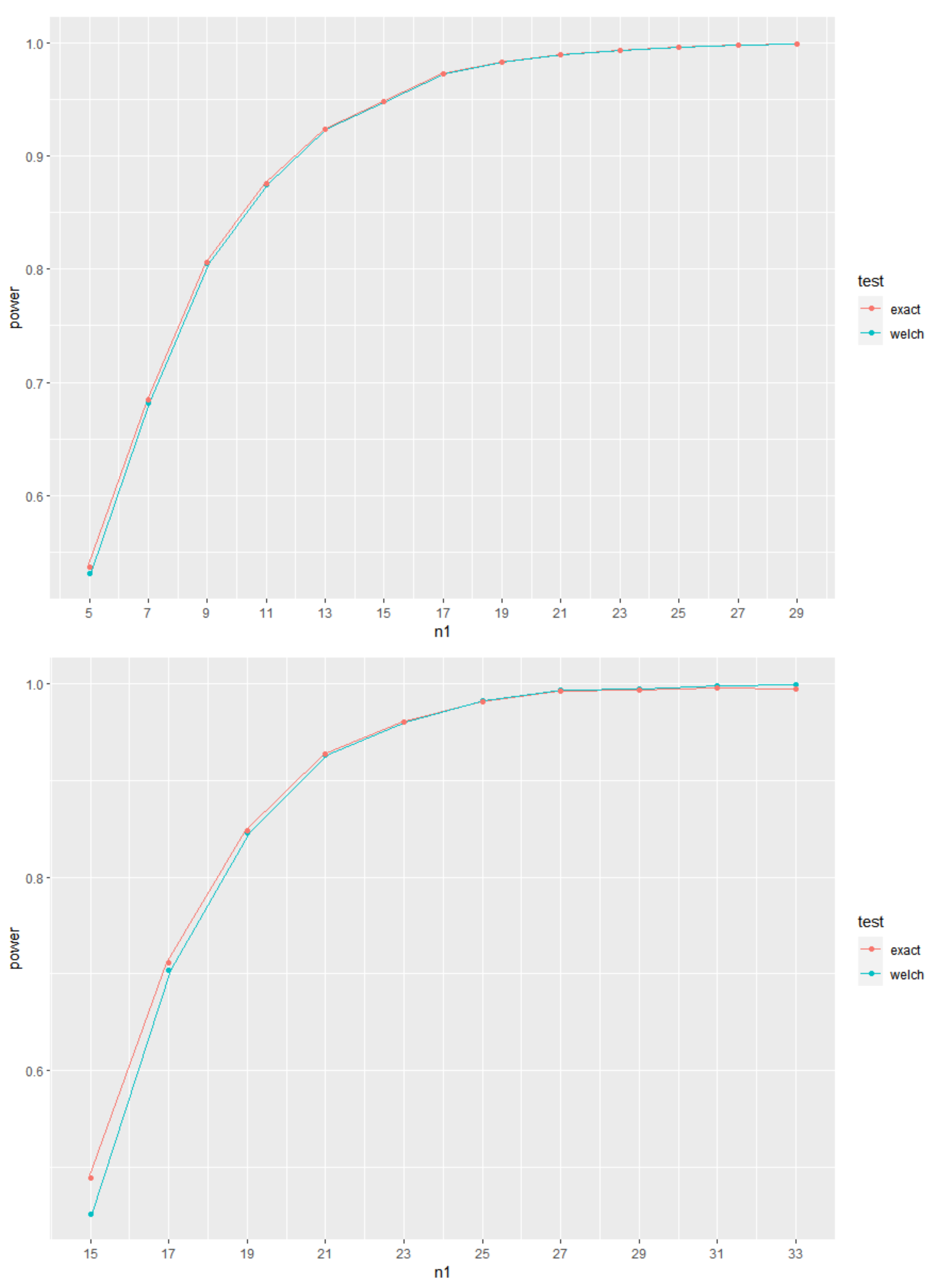
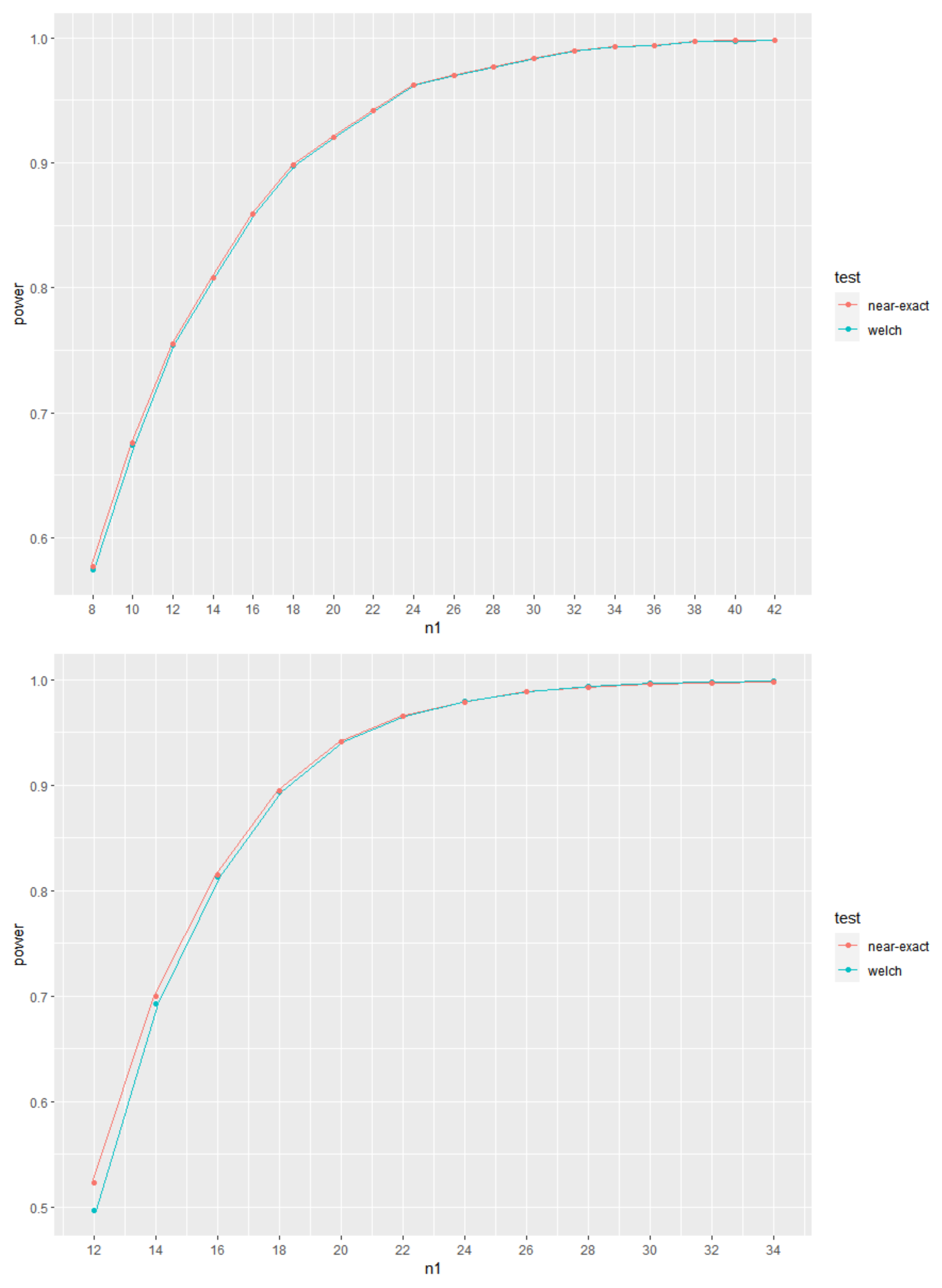
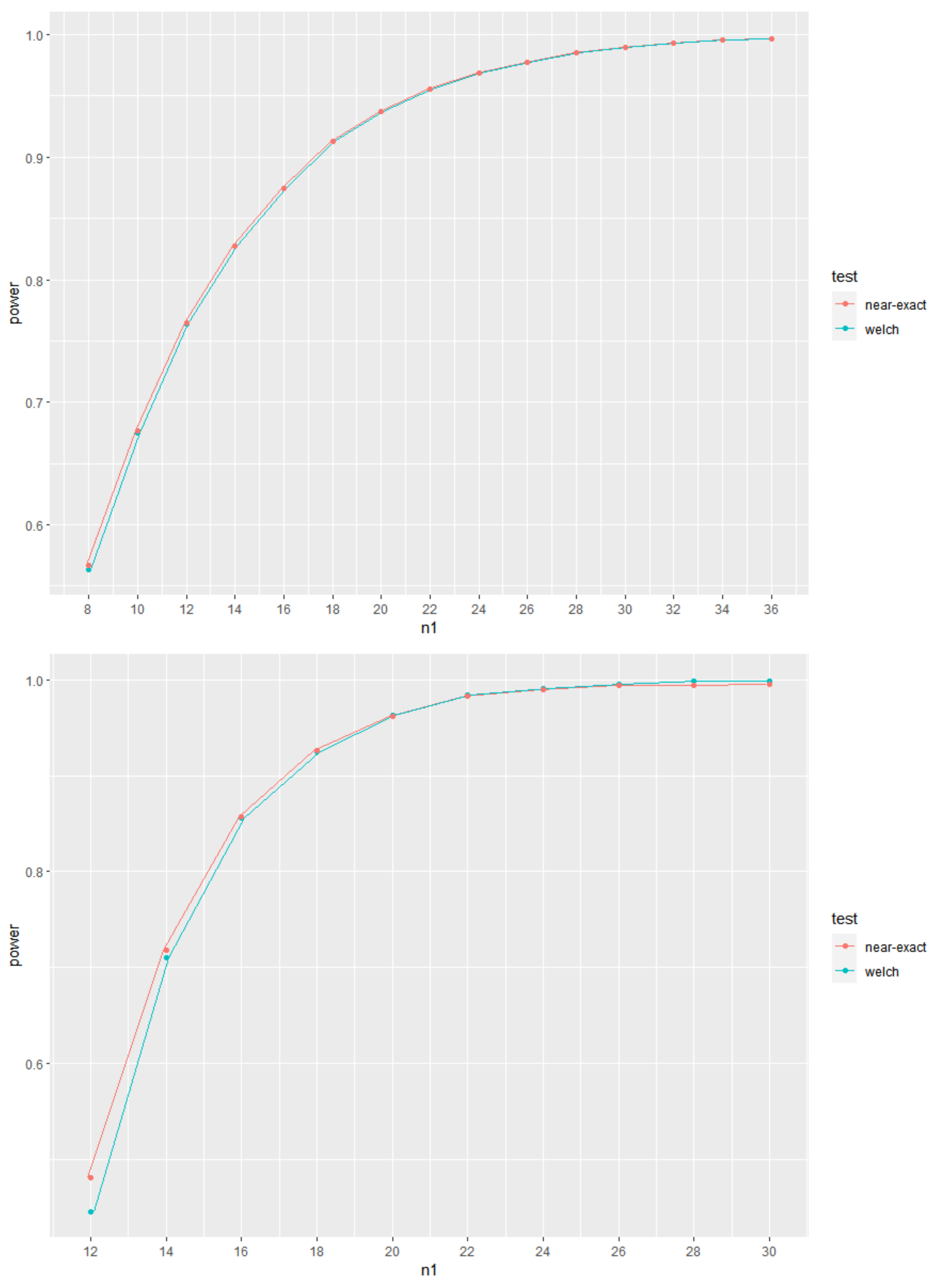
5.4. Brief Study of Power Evolution for Increasing Sample Sizes

With the aim of showing the evolution of the values of power for increasing sample sizes, the plots of power curves for increasing values of the sample sizes are shown in Figure 1, Figure 2 and Figure 3, for given ${\sigma }_1^2$, ${\sigma }_2^2$, ${\mu }_1$ and ${\mu }_2$. As expected, it is clear that the power curves are increasing with increasing values of the sample sizes. Figure 1, Figure 2 and Figure 3 represent, respectively, cases of $(n_1,n_2)=(odd,odd)$, $(even,even)$ and $(even,odd)$. It is also clear from these Figures that, also as expected, although the use of the exact or near-exact distributions lead to an increase in the values of power, the power values from Welch’s test approach asymptotically those obtained when using the exact or near-exact distributions for increasing sample sizes. In Figure 1, Figure 2 and Figure 3, we use $({\mu }_1,{\mu }_2)=(\sqrt{40},0)$ and present the values of $({\sigma }_1^2,{\sigma }_2^2)$ and $(n_1,n_2)$ in each figure. In addition, the corresponding values of $\delta$ are also presented.

6. Conclusions

Over the years since the Behrens–Fisher problem was first introduced, many different solutions have been presented for the problem. In this paper, we propose another approach for the Behrens–Fisher problem that is based on a version of the exact distribution and near-exact distributions for its statistic, which are based on GIG (generalized integer gamma) distributions. Overall, the differences between the sizes of the near-exact distribution and Welch’s t-test are negligible, while the use of the exact or near-exact distributions provide powers that are larger than those provided by Welch’s t-test, mainly for the cases where the sample sizes and/or the variances are unbalanced, and namely when smaller sample sizes are associated with larger variances. The results thus show that, mainly for the cases of unbalanced sample sizes and/or unbalanced variances, the use of Welch’s t-test leads to some loss in power compared with the use of the exact or near-exact distributions developed, thus advising towards the use of these latter ones.

The computation of the exact or near-exact distributions poses absolutely no problems, even for large sample sizes, with the computation times remaining in the hundredths of a second for sample sizes in the order of a few hundreds.

In order to decide which distribution to use, the user may want to test the hypothesis ${\lambda }_1={\lambda }_2$. We may note that, given the definition of ${\lambda }_1$ and ${\lambda }_2$ in (3), testing that hypothesis is indeed equivalent to testinf the hypothesis

$$\frac{{\sigma }_2}{{\sigma }_1}\frac{n_1(n_1-1)}{n_2(n_2-1)}=1,$$

which may tested in as much the same way we run a test of equality of two variances based on two independent samples.