
Covariance Matrix Adaptation Evolution Strategy for Improving Machine Learning Approaches in Streamflow Prediction


 ,
,  ,
,  and
and 
Abstract
:1. Introduction
2. Materials and Methods
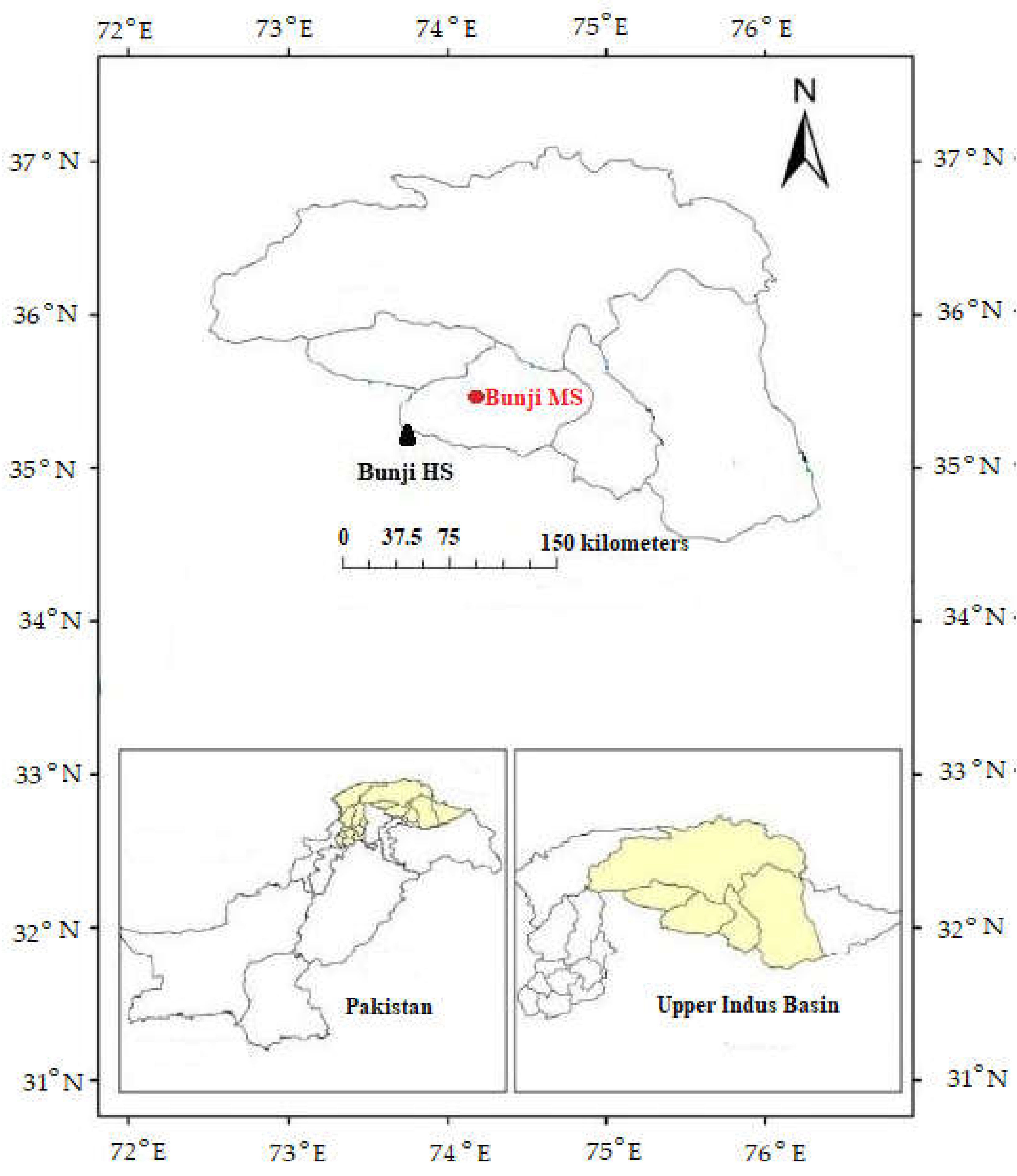
2.1. Study Region and Datasets
2.2. Streamflow Estimation Models
2.2.1. Elastic Net (EN)
2.2.2. Extreme Learning Machine (ELM)
2.2.3. Least Squares Support Vector Regression (LSSVR)
2.2.4. Support Vector Regression (SVR)
2.2.5. Radial Basis Function Neural Network (RBFNN)
2.2.6. eXtreme Gradient Boosting (XGB)
2.2.7. Gaussian Processes Regression (GPR)
2.3. Parameter Tuning Guided by a CMAES
| Algorithm 1. Pseudocode of the CMAES searches the internal parameters of the machine learning models. |
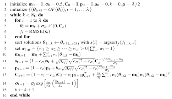 |
2.4. Performance Metrics
3. Results and Discussion
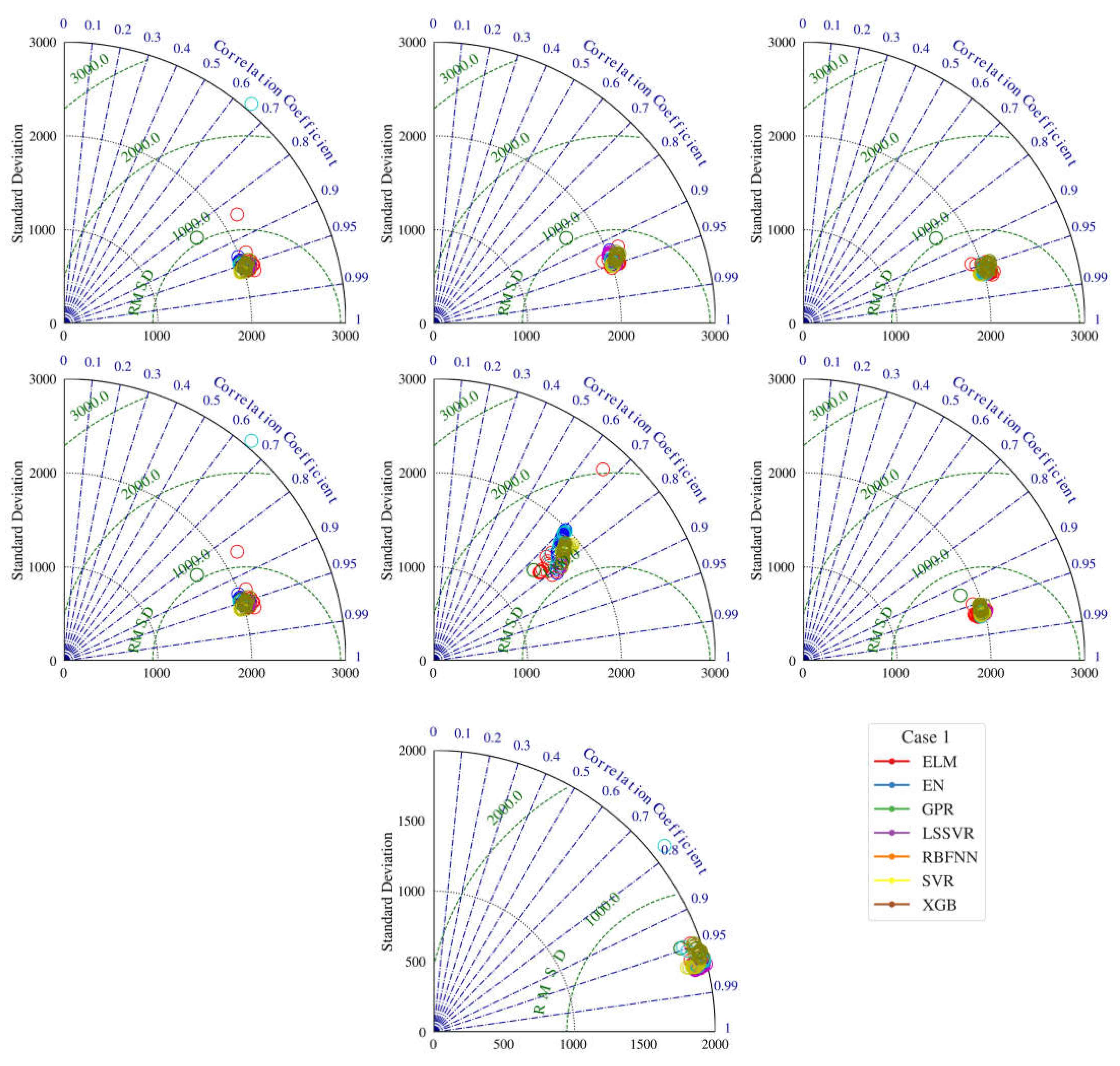
3.1. Results
3.2. Uncertainty Analysis
3.3. Discussion
4. Conclusions
- -
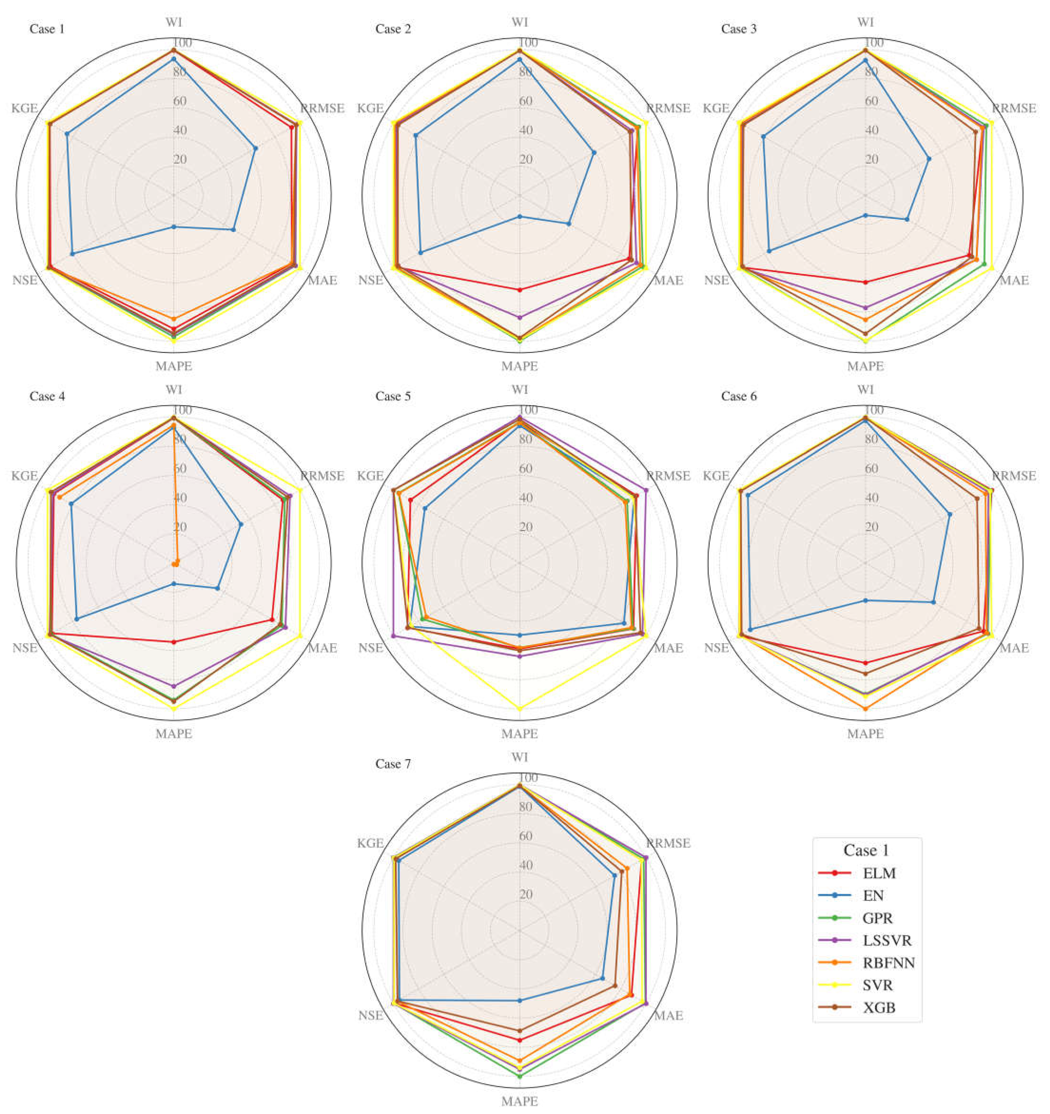
- This research evaluated the feasibility of seven hybrid machine learning methods in monthly streamflow forecasting. In the hybridization process, the metaheuristic covariance matrix adaptation evolution strategy assisted in adjusting the internal parameters of the models. In addition, an uncertainty analysis was performed on the resulting models. Methods were compared to each other considering the several metrics (e.g., WI, RRMSE, MAE, MAPE, NSE, and KGE together with standard deviation) and visual methods, such as radar chart, scatter, and Taylor diagrams. Seven input cases were taken into account, including temperature and discharge data. All the implemented methods provided better efficiency for discharge input cases, while temperature input cases also produced promising predictions. Among the implemented methods, the SVR generally performed superior to the other methods, especially for the temperature input cases. In contrast, the LSSVR and GPR were found to do better than the SVR in some discharge input cases. The EN method provided the worst streamflow predictions, according to all evaluation statistics and visual comparison. Uncertainty analysis revealed that the SVR generally has low uncertainty compared to other machine learning methods and the EN has the lowest uncertainty. Overall, temperature-based SVR models are highly recommended in monthly streamflow prediction. These outcomes are very useful in practical applications, especially in developing countries. Temperature data are easily measured, and the models that only use such data will be very beneficial for streamflow predictions in the basins where streamflow data are missing because of technical/economic reasons. The main limitation of this study is the use of limited data from one location. More data from different climatic regions are required to justify the accuracy of the proposed models. The covariance matrix adaptation evolution strategy was successfully applied for improving the accuracy of the ELM, EN, GPR, LSSVR, RBFNN, SVR, and XGB methods. This strategy can also be employed for other machine learning methods, such as ANN, ANFIS, and deep learning in future studies.
Author Contributions
Funding
Institutional Review Board Statement
Informed Consent Statement
Data Availability Statement
Conflicts of Interest
References
- Erdal, H.I.; Karakurt, O. Advancing monthly streamflow prediction accuracy of CART models using ensemble learning paradigms. J. Hydrol. 2013, 477, 119–128. [Google Scholar] [CrossRef]
- Yaseen, Z.M.; El-Shafie, A.; Jaafar, O.; Afan, H.A.; Sayl, K.N. Artificial intelligence based models for stream-flow forecasting: 2000–2015. J. Hydrol. 2015, 530, 829–844. [Google Scholar] [CrossRef]
- Rasouli, K.; Hsieh, W.W.; Cannon, A.J. Daily streamflow forecasting by machine learning methods with weather and climate inputs. J. Hydrol. 2012, 414–415, 284–293. [Google Scholar] [CrossRef]
- Liu, Z.; Zhou, P.; Zhang, Y. A Probabilistic Wavelet–Support Vector Regression Model for Streamflow Forecasting with Rainfall and Climate Information Input. J. Hydrometeorol. 2015, 16, 2209–2229. [Google Scholar] [CrossRef]
- Adnan, R.M.; Liang, Z.; Trajkovic, S.; Zounemat-Kermani, M.; Li, B.; Kisi, O. Daily streamflow prediction using optimally pruned extreme learning machine. J. Hydrol. 2019, 577, 123981. [Google Scholar] [CrossRef]
- Kisi, O.; Heddam, S.; Keshtegar, B.; Piri, J.; Adnan, R.M. Predicting Daily Streamflow in a Cold Climate Using a Novel Data Mining Technique: Radial M5 Model Tree. Water 2022, 14, 1449. [Google Scholar] [CrossRef]
- Faye, C. Comparative Analysis of Meteorological Drought Based on the SPI and SPEI Indices; Ziguinchor University: Ziguinchor, Senegal, 2022. [Google Scholar]
- Dawson, C.; Wilby, R. An artificial neural network approach to rainfall-runoff modelling. Hydrol. Sci. J. 1998, 43, 47–66. [Google Scholar] [CrossRef]
- Demirel, M.C.; Venancio, A.; Kahya, E. Flow forecast by SWAT model and ANN in Pracana basin, Portugal. Adv. Eng. Softw. 2009, 40, 467–473. [Google Scholar] [CrossRef]
- Bhadra, A.; Bandyopadhyay, A.; Singh, R.; Raghuwanshi, N.S. Rainfall-Runoff Modeling: Comparison of Two Approaches with Different Data Requirements. Water Resour. Manag. 2010, 24, 37–62. [Google Scholar] [CrossRef]
- Sudheer, C.; Maheswaran, R.; Panigrahi, B.K.; Mathur, S. A hybrid SVM-PSO model for forecasting monthly streamflow. Neural Comput. Appl. 2014, 24, 1381–1389. [Google Scholar] [CrossRef]
- Raghavendra, N.S.; Deka, P.C. Support vector machine applications in the field of hydrology: A review. Appl. Soft Comput. 2014, 19, 372–386. [Google Scholar] [CrossRef]
- Nourani, V.; Baghanam, A.H.; Adamowski, J.; Kisi, O. Applications of hybrid wavelet–Artificial Intelligence models in hydrology: A review. J. Hydrol. 2014, 514, 358–377. [Google Scholar] [CrossRef]
- Ibrahim, K.S.M.H.; Huang, Y.F.; Ahmed, A.N.; Koo, C.H.; El-Shafie, A. A review of the hybrid artificial intelligence and optimization modelling of hydrological streamflow forecasting. Alex. Eng. J. 2021, 61, 279–303. [Google Scholar] [CrossRef]
- Kagoda, P.A.; Ndiritu, J.; Ntuli, C.; Mwaka, B. Application of radial basis function neural networks to short-term streamflow forecasting. Phys. Chem. Earth Parts A/B/C 2010, 35, 571–581. [Google Scholar] [CrossRef]
- Sun, A.Y.; Wang, D.; Xu, X. Monthly streamflow forecasting using Gaussian Process Regression. J. Hydrol. 2014, 511, 72–81. [Google Scholar] [CrossRef]
- Mehr, A.D.; Kahya, E.; Şahin, A.; Nazemosadat, M.J. Successive-station monthly streamflow prediction using different artificial neural network algorithms. Int. J. Environ. Sci. Technol. 2015, 12, 2191–2200. [Google Scholar] [CrossRef]
- Kisi, O. Streamflow Forecasting and Estimation Using Least Square Support Vector Regression and Adaptive Neuro-Fuzzy Embedded Fuzzy c-means Clustering. Water Resour. Manag. 2015, 29, 5109–5127. [Google Scholar] [CrossRef]
- Yaseen, Z.M.; Kisi, O.; Demir, V. Enhancing Long-Term Streamflow Forecasting and Predicting using Periodicity Data Component: Application of Artificial Intelligence. Water Resour. Manag. 2016, 30, 4125–4151. [Google Scholar] [CrossRef]
- Modaresi, F.; Araghinejad, S.; Ebrahimi, K. A Comparative Assessment of Artificial Neural Network, Generalized Regression Neural Network, Least-Square Support Vector Regression, and K-Nearest Neighbor Regression for Monthly Streamflow Forecasting in Linear and Nonlinear Conditions. Water Resour. Manag. 2018, 32, 243–258. [Google Scholar] [CrossRef]
- Worland, S.C.; Farmer, W.; Kiang, J.E. Improving predictions of hydrological low-flow indices in ungaged basins using machine learning. Environ. Model. Softw. 2018, 101, 169–182. [Google Scholar] [CrossRef]
- Hadi, S.J.; Abba, S.I.; Sammen, S.S.; Salih, S.Q.; Al-Ansari, N.; Yaseen, Z.M. Non-Linear Input Variable Selection Approach Integrated With Non-Tuned Data Intelligence Model for Streamflow Pattern Simulation. IEEE Access 2019, 7, 141533–141548. [Google Scholar] [CrossRef]
- Li, Y.; Liang, Z.; Hu, Y.; Li, B.; Xu, B.; Wang, D. A multi-model integration method for monthly streamflow prediction: Modified stacking ensemble strategy. J. Hydroinform. 2020, 22, 310–326. [Google Scholar] [CrossRef]
- Ni, L.; Wang, D.; Wu, J.; Wang, Y.; Tao, Y.; Zhang, J.; Liu, J. Streamflow forecasting using extreme gradient boosting model coupled with Gaussian mixture model. J. Hydrol. 2020, 586, 124901. [Google Scholar] [CrossRef]
- Adnan, R.M.; Liang, Z.; Heddam, S.; Zounemat-Kermani, M.; Kisi, O.; Li, B. Least square support vector machine and multivariate adaptive regression splines for streamflow prediction in mountainous basin using hydro-meteorological data as inputs. J. Hydrol. 2020, 586, 124371. [Google Scholar] [CrossRef]
- Thapa, S.; Zhao, Z.; Li, B.; Lu, L.; Fu, D.; Shi, X.; Tang, B.; Qi, H. Snowmelt-Driven Streamflow Prediction Using Machine Learning Techniques (LSTM, NARX, GPR, and SVR). Water 2020, 12, 1734. [Google Scholar] [CrossRef]
- Jiang, Y.; Bao, X.; Hao, S.; Zhao, H.; Li, X.; Wu, X. Monthly Streamflow Forecasting Using ELM-IPSO Based on Phase Space Reconstruction. Water Resour. Manag. 2020, 34, 3515–3531. [Google Scholar] [CrossRef]
- Malik, A.; Tikhamarine, Y.; Souag-Gamane, D.; Kisi, O.; Pham, Q.B. Support vector regression optimized by meta-heuristic algorithms for daily streamflow prediction. Stoch. Hydrol. Hydraul. 2020, 34, 1755–1773. [Google Scholar] [CrossRef]
- Parisouj, P.; Mohebzadeh, H.; Lee, T. Employing Machine Learning Algorithms for Streamflow Prediction: A Case Study of Four River Basins with Different Climatic Zones in the United States. Water Resour. Manag. 2020, 34, 4113–4131. [Google Scholar] [CrossRef]
- Niu, W.-J.; Feng, Z.-K. Evaluating the performances of several artificial intelligence methods in forecasting daily streamflow time series for sustainable water resources management. Sustain. Cities Soc. 2021, 64, 102562. [Google Scholar] [CrossRef]
- Jiang, Q.; Cheng, Y.; Le, H.; Li, C.; Liu, P.X. A Stacking Learning Model Based on Multiple Similar Days for Short-Term Load Forecasting. Mathematics 2022, 10, 2446. [Google Scholar] [CrossRef]
- Yang, C.-H.; Shao, J.-C.; Liu, Y.-H.; Jou, P.-H.; Lin, Y.-D. Application of Fuzzy-Based Support Vector Regression to Forecast of International Airport Freight Volumes. Mathematics 2022, 10, 2399. [Google Scholar] [CrossRef]
- Su, H.; Peng, X.; Liu, H.; Quan, H.; Wu, K.; Chen, Z. Multi-Step-Ahead Electricity Price Forecasting Based on Temporal Graph Convolutional Network. Mathematics 2022, 10, 2366. [Google Scholar] [CrossRef]
- De-Prado-Gil, J.; Zaid, O.; Palencia, C.; Martínez-García, R. Prediction of Splitting Tensile Strength of Self-Compacting Recycled Aggregate Concrete Using Novel Deep Learning Methods. Mathematics 2022, 10, 2245. [Google Scholar] [CrossRef]
- Samadianfard, S.; Jarhan, S.; Salwana, E.; Mosavi, A.; Shamshirband, S.; Akib, S. Support Vector Regression Integrated with Fruit Fly Optimization Algorithm for River Flow Forecasting in Lake Urmia Basin. Water 2019, 11, 1934. [Google Scholar] [CrossRef]
- Tikhamarine, Y.; Souag-Gamane, D.; Kisi, O. A new intelligent method for monthly streamflow prediction: Hybrid wavelet support vector regression based on grey wolf optimizer (WSVR–GWO). Arab. J. Geosci. 2019, 12, 540. [Google Scholar] [CrossRef]
- Hansen, N.; Müller, S.D.; Koumoutsakos, P. Reducing the Time Complexity of the Derandomized Evolution Strategy with Covariance Matrix Adaptation (CMA-ES). Evol. Comput. 2003, 11, 1–18. [Google Scholar] [CrossRef]
- Rouchier, S.; Woloszyn, M.; Kedowide, Y.; Bejat, T. Identification of the hygrothermal properties of a building envelope material by the covariance matrix adaptation evolution strategy. J. Build. Perform. Simul. 2016, 9, 101–114. [Google Scholar] [CrossRef]
- Liang, Y.; Wang, X.; Zhao, H.; Han, T.; Wei, Z.; Li, Y. A covariance matrix adaptation evolution strategy variant and its engineering application. Appl. Soft Comput. 2019, 83, 105680. [Google Scholar] [CrossRef]
- Chen, G.; Li, S.; Wang, X. Source mask optimization using the covariance matrix adaptation evolution strategy. Opt. Express 2020, 28, 33371–33389. [Google Scholar] [CrossRef]
- Kaveh, A.; Javadi, S.M.; Moghanni, R.M. Reliability Analysis via an Optimal Covariance Matrix Adaptation Evolution Strategy: Emphasis on Applications in Civil Engineering. Period. Polytech. Civ. Eng. 2020, 64, 579–588. [Google Scholar] [CrossRef]
- Hastie, T.; Tibshirani, R.; Friedman, J.H.; Friedman, J.H. The Elements of Statistical Learning-Data Mining, Inference, and Prediction, 2nd ed.; Springer: New York, NY, USA, 2009. [Google Scholar]
- Zou, H.; Hastie, T. Regularization and Variable Selection via the Elastic Net. J. R. Stat. Soc. 2005, 67, 301–320. [Google Scholar] [CrossRef]
- Guo, P.; Cheng, W.; Wang, Y. Hybrid evolutionary algorithm with extreme machine learning fitness function evaluation for two-stage capacitated facility location problems. Expert Syst. Appl. 2017, 71, 57–68. [Google Scholar] [CrossRef]
- Saporetti, C.M.; Duarte, G.R.; Fonseca, T.L.; Da Fonseca, L.G.; Pereira, E. Extreme Learning Machine combined with a Differential Evolution algorithm for lithology identification. RITA 2018, 25, 43–56. [Google Scholar] [CrossRef]
- Huang, G.; Huang, G.-B.; Song, S.; You, K. Trends in extreme learning machines: A review. Neural Netw. 2015, 61 (Suppl. C), 32–48. [Google Scholar] [CrossRef]
- Suykens, J.A.K.; Vandewalle, J. Least Squares Support Vector Machine Classifiers. Neural Process. Lett. 1999, 9, 293–300. [Google Scholar] [CrossRef]
- Chang, C.C.; Lin, C.J. LIBSVM: A Library for Support Vector Machines. ACM Trans. Intell. Syst. Technol. 2011, 2, 1–27. [Google Scholar] [CrossRef]
- Karthikeyan, M.; Vyas, R. Machine learning methods in chemoinformatics for drug discovery. In Practical Chemoinformatics; Springer: Berlin/Heidelberg, Germany, 2014; pp. 133–194. [Google Scholar] [CrossRef]
- Gunn, S.R. Support Vector Machines for Classification and Regression. ISIS Tech. Rep. 1998, 14, 5–16. [Google Scholar]
- Kargar, K.; Samadianfard, S.; Parsa, J.; Nabipour, N.; Shamshirband, S.; Mosavi, A.; Chau, K.-W. Estimating longitudinal dispersion coefficient in natural streams using empirical models and machine learning algorithms. Eng. Appl. Comput. Fluid Mech. 2020, 14, 311–322. [Google Scholar] [CrossRef]
- Broomhead, D.S.; Lowe, D. Radial basis functions, multi-variable functional interpolation and adaptive networks. In Royal Signals; Radar Establishment Malvern: Malvern, UK, 1988. [Google Scholar]
- Chen, T.; Guestrin, C. XGBoost: A Scalable Tree Boosting System. In Proceedings of the 22nd ACM Sigkdd International Conference on Knowledge Discovery and Data Mining, San Francisco, CA, USA, 13–17 August 2016; KDD’16. ACM: New York, NY, USA, 2016; pp. 785–794. [Google Scholar]
- Chen, T.; He, T. Higgs boson discovery with boosted trees. In NIPS 2014 Workshop on High-Energy Physics and Machine Learning; PMLR: London, UK, 2015; pp. 69–80. [Google Scholar]
- Ou, X.; Morris, J.; Martin, E. Gaussian Process Regression for Batch Process Modelling. IFAC Proc. Vol. 2004, 37, 817–822. [Google Scholar] [CrossRef]
- Wang, B.; Chen, T. Gaussian process regression with multiple response variables. Chemom. Intell. Lab. Syst. 2015, 142, 159–165. [Google Scholar] [CrossRef]
- Schulz, E.; Speekenbrink, M.; Krause, A. A Tutorial on Gaussian Process Regression: Modelling, Exploring, and Exploiting Functions. J. Math. Psychol. 2018, 85, 1–16. [Google Scholar] [CrossRef]
- Kumar, R. The generalized modified Bessel function and its connection with Voigt line profile and Humbert functions. Adv. Appl. Math. 2020, 114, 101986. [Google Scholar] [CrossRef]
- Hansen, N.; Ostermeier, A. Completely Derandomized Self-Adaptation in Evolution Strategies. Evol. Comput. 2001, 9, 159–195. [Google Scholar] [CrossRef] [PubMed]
- Beyer, H.G.; Schwefel, H.P. Evolution Strategies–a Comprehensive Introduction. Nat. Comput. 2002, 1, 3–52. [Google Scholar] [CrossRef]
- Li, Z.; Zhang, Q.; Lin, X.; Zhen, H.-L. Fast Covariance Matrix Adaptation for Large-Scale Black-Box Optimization. IEEE Trans. Cybern. 2018, 50, 2073–2083. [Google Scholar] [CrossRef]
- Willmott, C.J. ON the Validation of Models. Phys. Geogr. 1981, 2, 184–194. [Google Scholar] [CrossRef]
- Nash, J.E.; Sutcliffe, J.V. River flow forecasting through conceptual models part I—A discussion of principles. J. Hydrol. 1970, 10, 282–290. [Google Scholar] [CrossRef]
- Gupta, H.V.; Kling, H.; Yilmaz, K.K.; Martinez, G.F. Decomposition of the mean squared error and NSE performance criteria: Implications for improving hydrological modelling. J. Hydrol. 2009, 377, 80–91. [Google Scholar] [CrossRef]
- Kisi, O.; Shiri, J.; Karimi, S.; Adnan, R.M. Three different adaptive neuro fuzzy computing techniques for forecasting long-period daily streamflows. In Big Data in Engineering Applications; Springer: Singapore, 2018; pp. 303–321. [Google Scholar] [CrossRef]
- Alizamir, M.; Kisi, O.; Adnan, R.M.; Kuriqi, A. Modelling reference evapotranspiration by combining neuro-fuzzy and evolutionary strategies. Acta Geophys. 2020, 68, 1113–1126. [Google Scholar] [CrossRef]
- Yuan, X.; Chen, C.; Lei, X.; Yuan, Y.; Muhammad Adnan, R. Monthly runoff forecasting based on LSTM–ALO model. Stoch. Environ. Res. Risk Assess. 2018, 32, 2199–2212. [Google Scholar] [CrossRef]
- Sattar, A.M.; Gharabaghi, B. Gene expression models for prediction of longitudinal dispersion coefficient in streams. J. Hydrol. 2015, 524, 587–596. [Google Scholar] [CrossRef]
- Sudheer, K.P.; Gosain, A.K.; Ramasastri, K.S. A data-driven algorithm for constructing artificial neural network rainfall-runoff models. Hydrol. Process. 2002, 16, 1325–1330. [Google Scholar] [CrossRef]
- Kisi, O. Constructing neural network sediment estimation models using a data-driven algorithm. Math. Comput. Simul. 2008, 79, 94–103. [Google Scholar] [CrossRef]
- Wu, C.; Chau, K. Prediction of rainfall time series using modular soft computingmethods. Eng. Appl. Artif. Intell. 2013, 26, 997–1007. [Google Scholar] [CrossRef]
- Adnan, R.M.; Liang, Z.; Parmar, K.S.; Soni, K.; Kisi, O. Modeling monthly streamflow in mountainous basin by MARS, GMDH-NN and DENFIS using hydroclimatic data. Neural Comput. Appl. 2021, 33, 2853–2871. [Google Scholar] [CrossRef]


| Dataset | Parameter | Min | Mean | Std | Max |
|---|---|---|---|---|---|
| Training | T (C) | −3.33 | 13.80 | 8.72 | 29.45 |
| Q (m/s) | 251.72 | 1784.68 | 1971.37 | 7799.4 | |
| Test | T (C) | −1.22 | 14.15 | 9.03 | 28.65 |
| Q (m/s) | 272.50 | 1844.64 | 1941.29 | 1941.29 |
| Case. | Input Features |
|---|---|
| Case 1 | |
| Case 2 | |
| Case 3 | |
| Case 4 | |
| Case 5 | |
| Case 6 | |
| Case 7 |
| # | Name | |
|---|---|---|
| 1 | Identity | |
| 2 | Sigmoid | |
| 3 | Hyperbolic tangent | |
| 4 | Gaussian | |
| 5 | Swish | |
| 6 | ReLU |
| # | Name | |
|---|---|---|
| 1 | Linear | |
| 2 | Multiquadrics | |
| 3 | Inverse multiquadrics | |
| 4 | Gaussian | |
| 5 | Cubic | |
| 6 | Quintic | |
| 7 | Thin plate |
| Method | IP | Description | Settings/Range |
|---|---|---|---|
| ELM | q1 | No. neurons in the hidden layer | [1, 500] |
| q2 | Regularization parameter, C | [0.0001, 10,000] | |
| q3 | Activation function, G | 1: Identity; 2: Sigmoid; 3: Hyperbolic Tangent; 4: Gaussian; 5: Swish; 6: ReLU; | |
| EN | q1 | Penalty term, a | [10−6, 1] |
| q2 | L1-ratio parameter, r | [0, 1] | |
| GPR | q1 | Kernel parameter, k0 | [0.001, 10] |
| q2 | Kernel parameter, n | [0.001, 10] | |
| q3 | Kernel parameter, k0 | [0, 100] | |
| q4 | Regularization parameter, a | [10−8, 1] | |
| LSSVR | q1 | Regularization parameter, C | [1, 1000] |
| q2 | Bandwidth parameter, g | 0.001, 100] | |
| RBFNN | q1 | Activation function width, e | [1, 500] |
| q2 | Smoothing parameter, l | [0.0001, 10,000] | |
| q3 | Activation function, f | 1: Linear; 2: Multiquadric; 3: Inverse Multiquadric; 4: Gaussian; 5: Cubic; 6: Quintic; 7: Thin Plate; | |
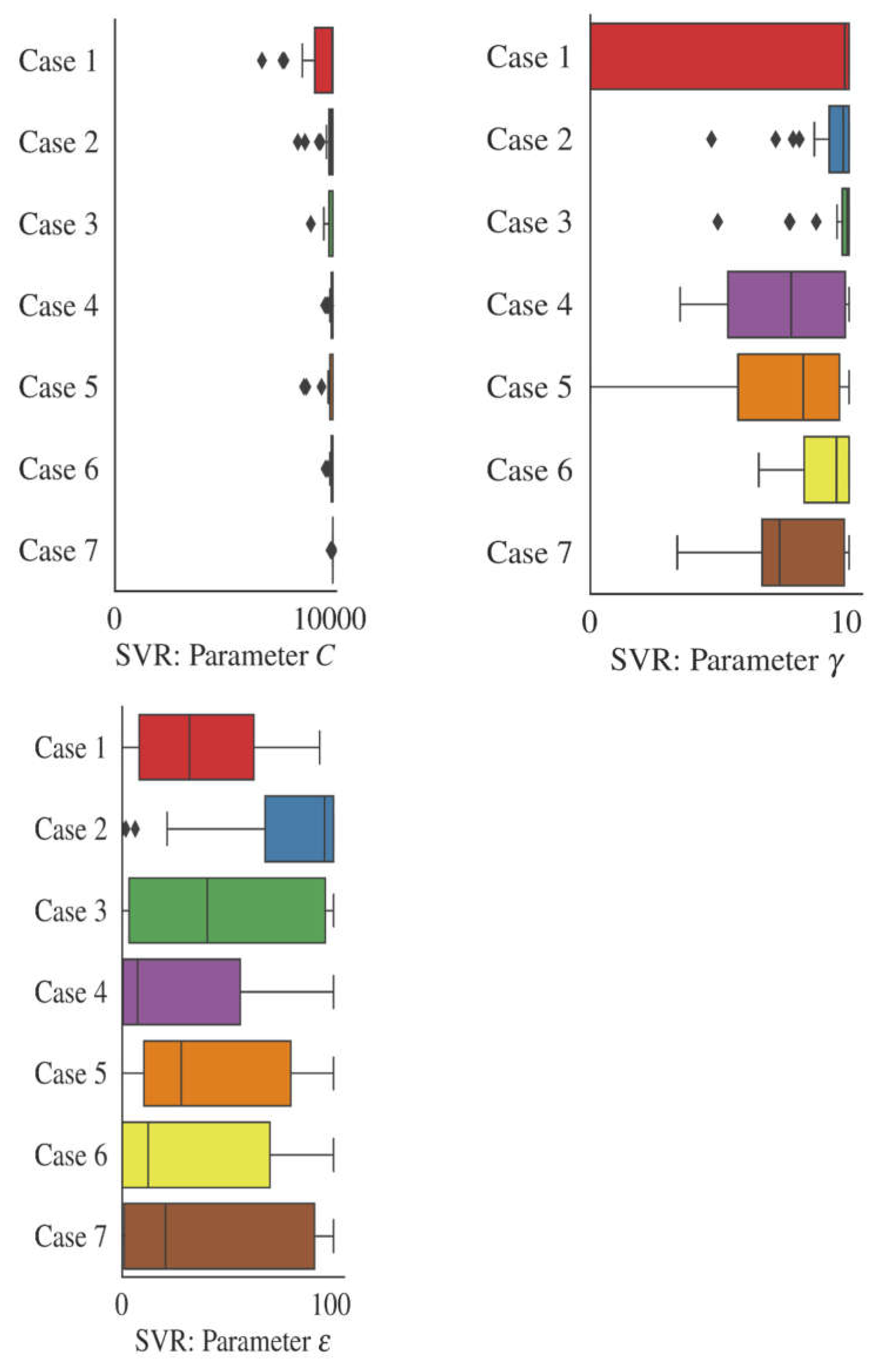
| SVR | q1 | Loss parameter, e | [10−5, 1] |
| q2 | Regularization parameter, C | [1, 10,000] | |
| q3 | Bandwidth parameter, g | [0.001, 10] | |
| XGB | q1 | Learning rate, l | [10−6, 1] |
| q2 | No. weak estimators, Mest | [10, 500] | |
| q3 | Maximum depth, mdepth | [1, 20] | |
| q4 | Regularization parameter, lreg | [0, 100] |
| Metric Acronym | Expression |
|---|---|
| MAE | |
| MAPE | |
| NSE | |
| KGE | |
| WI | |
| RRMSE |
| Estimator | WI | RRMSE | MAE | MAPE | NSE | Kq + GE |
|---|---|---|---|---|---|---|
| ELM | 0.965 (0.007) | 0.402 (0.044) | 441.44 (26.13) | 28.28 (3.500) | 0.855 (0.037) | 0.898 (0.025) |
| EN | 0.908 (0.000) | 0.578 (0.000) | 875.05 (0.000) | 120.11 (0.000) | 0.703 (0.000) | 0.774 (0.000) |
| GPR | 0.968 (0.001) | 0.385 (0.008) | 427.99 (10.56) | 26.69 (0.300) | 0.868 (0.005) | 0.904 (0.003) |
| LSSVR | 0.968 (0.001) | 0.385 (0.007) | 428.95 (11.08) | 27.18 (0.726) | 0.869 (0.005) | 0.904 (0.002) |
| RBFNN | 0.968 (0.004) | 0.387 (0.022) | 442.57 (53.73) | 30.55 (10.98) | 0.867 (0.017) | 0.904 (0.007) |
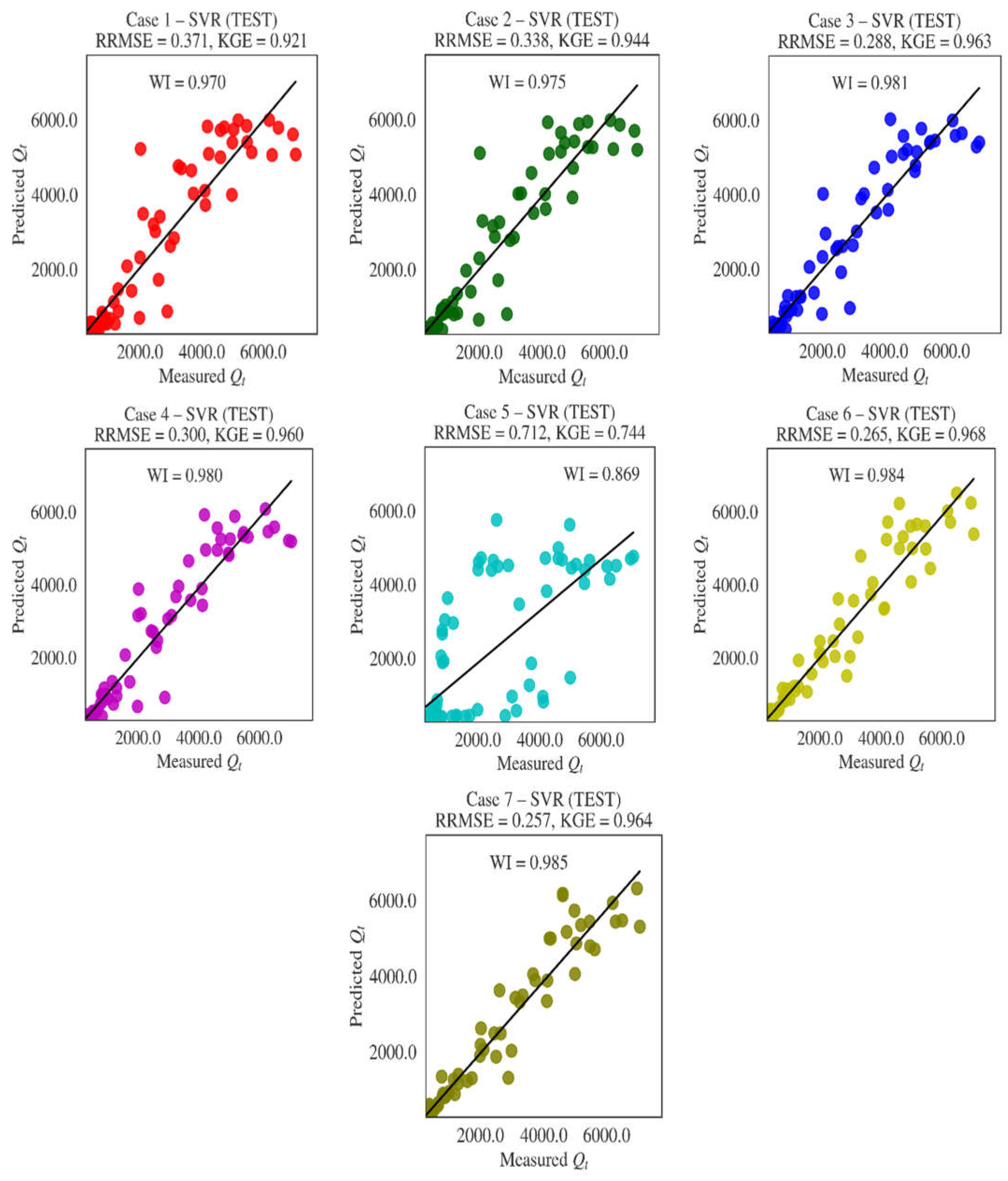
| SVR | 0.970 (0.000) | 0.375 (0.003) | 412.98 (4.13) | 25.91 (0.620) | 0.876 (0.002) | 0.915 (0.004) |
| XGB | 0.968 (0.002) | 0.387 (0.012) | 434.24 (14.39) | 27.37 (0.534) | 0.867 (0.009) | 0.898 (0.011) |
| Estimator | WI | RRMSE | MAE | MAPE | NSE | KGE |
|---|---|---|---|---|---|---|
| ELM | 0.971 (0.004) | 0.363 (0.022) | 394.59 (42.45) | 26.54 (8.130) | 0.883 (0.015) | 0.922 (0.013) |
| EN | 0.909 (0.000) | 0.577 (0.000) | 881.96 (0.000) | 118.81 (0.000) | 0.704 (0.000) | 0.777 (0.000) |
| GPR | 0.971 (0.004) | 0.360 (0.023) | 350.88 (14.52) | 17.21 (1.540) | 0.884 (0.015) | 0.932 (0.010) |
| LSSVR | 0.968 (0.005) | 0.382 (0.026) | 369.83 (10.97) | 20.53 (1.300) | 0.870 (0.018) | 0.921 (0.003) |
| RBFNN | 0.971 (0.001) | 0.366 (0.009) | 358.07 (9.61) | 17.40 (0.438) | 0.881 (0.006) | 0.932 (0.002) |
| SVR | 0.975 (0.00) | 0.339 (0.003) | 342.25 (5.11) | 17.36 (0.646) | 0.898 (0.002) | 0.943 (0.002) |
| XGB | 0.968 (0.002) | 0.389 (0.015) | 386.32 (19.42) | 17.61 (0.987) | 0.866 (0.010) | 0.909 (0.009) |
| Estimator | WI | RRMSE | MAE | MAPE | NSE | KGE |
|---|---|---|---|---|---|---|
| ELM | 0.979 (0.003) | 0.313 (0.021) | 352.43 (40.86) | 27.06 (6.670) | 0.913 (0.012) | 0.929 (0.011) |
| EN | 0.910 (0.000) | 0.575 (0.000) | 879.59 (0.003) | 118.37 (0.001) | 0.707 (0.000) | 0.778 (0.000) |
| GPR | 0.980 (0.001) | 0.303 (0.009) | 307.32 (13.57) | 16.12 (1.730) | 0.918 (0.005) | 0.947 (0.007) |
| LSSVR | 0.979 (0.002) | 0.310 (0.013) | 328.71 (21.43) | 20.91 (1.880) | 0.915 (0.007) | 0.938 (0.004) |
| RBFNN | 0.978 (0.002) | 0.314 (0.015) | 328.96 (34.73) | 18.91 (8.270) | 0.913 (0.009) | 0.947 (0.009) |
| SVR | 0.981 (0.00) | 0.290 (0.001) | 289.21 (5.09) | 16.19 (0.669) | 0.925 (0.00) | 0.962 (0.001) |
| XGB | 0.976 (0.003) | 0.333 (0.019) | 342.84 (23.62) | 16.99 (1.520) | 0.902 (0.011) | 0.928 (0.012) |
| Estimator | WI | RRMSE | MAE | MAPE | NSE | KGE |
|---|---|---|---|---|---|---|
| ELM | 0.972 (0.012) | 0.356 (0.063) | 394.67 (36.17) | 31.46 (8.530) | 0.884 (0.053) | 0.908 (0.026) |
| EN | 0.909 (0.000) | 0.578 (0.000) | 885.37 (0.000) | 119.59 (0.000) | 0.704 (0.000) | 0.777 (0.000) |
| GPR | 0.973 (0.002) | 0.350 (0.014) | 358.39 (17.63) | 18.14 (2.580) | 0.891 (0.009) | 0.931 (0.014) |
| LSSVR | 0.976 (0.000) | 0.334 (0.006) | 347.08 (5.79) | 20.15 (1.150) | 0.901 (0.004) | 0.915 (0.005) |
| RBFNN | 0.925 (0.192) | 0.900 (0.620) | 376.58 (6.103) | 21.21 (9490.7) | 0.876 (0.005) | 0.864 (0.309) |
| SVR | 0.979 (0.000) | 0.308 (0.003) | 307.08 (5.060) | 17.06 (0.820) | 0.916 (0.002) | 0.956 (0.002) |
| XGB | 0.975 (0.002) | 0.340 (0.017) | 364.48 (22.67) | 17.95 (2.210) | 0.897 (0.010) | 0.930 (0.012) |
| Estimator | WI | RRMSE | MAE | MAPE | NSE | KGE |
|---|---|---|---|---|---|---|
| ELM | 0.858 (0.020) | 0.700 (0.090) | 915.48 (45.45) | 71.82 (2.850) | 0.558 (0.142) | 0.647 (0.052) |
| EN | 0.834 (0.000) | 0.715 (0.000) | 999.14 (0.000) | 85.40 (0.000) | 0.547 (0.000) | 0.562 (0.000) |
| GPR | 0.854 (0.013) | 0.761 (0.053) | 919.25 (33.68) | 72.80 (2.110) | 0.484 (0.068) | 0.718 (0.008) |
| LSSVR | 0.887 (0.001) | 0.647 (0.006) | 848.64 (5.78) | 65.94 (0.455) | 0.628 (0.007) | 0.748 (0.002) |
| RBFNN | 0.851 (0.011) | 0.775 (0.048) | 931.38 (27.37) | 72.58 (3.280) | 0.465 (0.063) | 0.715 (0.009) |
| SVR | 0.871 (0.002) | 0.719 (0.004) | 825.33 (13.78) | 42.27 (3.210) | 0.541 (0.005) | 0.746 (0.004) |
| XGB | 0.873 (0.007) | 0.707 (0.030) | 862.83 (14.08) | 70.24 (1.310) | 0.556 (0.036) | 0.747 (0.004) |
| Estimator | WI | RRMSE | MAE | MAPE | NSE | KGE |
|---|---|---|---|---|---|---|
| ELM | 0.983 (0.002) | 0.273 (0.017) | 303.21 (26.09) | 17.69 (3.960) | 0.934 (0.009) | 0.958 (0.007) |
| EN | 0.959 (0.000) | 0.409 (0.000) | 527.22 (0.000) | 47.25 (0.000) | 0.852 (0.000) | 0.893 (0.000) |
| GPR | 0.983 (0.00) | 0.275 (0.007) | 292.42 (3.24) | 13.49 (0.306) | 0.933 (0.003) | 0.950 (0.005) |
| LSSVR | 0.983 (0.00) | 0.280 (0.007) | 294.22 (3.01) | 13.41 (0.416) | 0.930 (0.003) | 0.948 (0.004) |
| RBFNN | 0.982 (0.001) | 0.287 (0.011) | 295.48 (7.48) | 12.14 (0.594) | 0.927 (0.005) | 0.956 (0.002) |
| SVR | 0.983 (0.00) | 0.277 (0.004) | 283.49 (4.91) | 13.24 (1.030) | 0.932 (0.002) | 0.960 (0.00400) |
| XGB | 0.979 (0.002) | 0.309 (0.015) | 315.66 (15.48) | 15.98 (1.900) | 0.915 (0.008) | 0.948 (0.007) |
| Estimator | WI | RRMSE | MAE | MAPE | NSE | KGE |
|---|---|---|---|---|---|---|
| ELM | 0.984 (0.003) | 0.266 (0.019) | 288.71 (14.91) | 15.54 (1.690) | 0.937 (0.010) | 0.962 (0.005) |
| EN | 0.972 (0.000) | 0.341 (0.000) | 389.77 (0.000) | 24.34 (0.000) | 0.897 (0.000) | 0.926 (0.000) |
| GPR | 0.985 (0.00) | 0.261 (0.009) | 256.68 (9.810) | 11.69 (0.597) | 0.939 (0.004) | 0.967 (0.003) |
| LSSVR | 0.985 (0.00) | 0.256 (0.007) | 255.54 (13.78) | 12.28 (1.310) | 0.942 (0.003) | 0.966 (0.003) |
| RBFNN | 0.978 (0.020) | 0.301 (0.092) | 293.20 (70.77) | 13.11 (4.670) | 0.912 (0.082) | 0.950 (0.039) |
| SVR | 0.984 (0.00) | 0.266 (0.009) | 263.44 (7.080) | 12.44 (0.715) | 0.937 (0.004) | 0.962 (0.006) |
| XGB | 0.977 (0.002) | 0.317 (0.017) | 338.54 (27.27) | 17.01 (3.410) | 0.910 (0.009) | 0.949 (0.006) |
| Model | Case | Mean Prediction Error | Width of Uncertainty Band | 95% Prediction Error Interval |
|---|---|---|---|---|
| ELM | Case 1 | −0.009 | 0.157 | 0.502 to 2.07 |
| Case 2 | −0.031 | 0.154 | 0.535 to 2.15 | |
| Case 3 | −0.027 | 0.176 | 0.481 to 2.36 | |
| Case 4 | −0.034 | 0.157 | 0.533 to 2.19 | |
| Case 5 | +0.061 | 0.320 | 0.205 to 3.68 | |
| Case 6 | +0.013 | 0.085 | 0.663 to 1.42 | |
| Case 7 | +0.009 | 0.074 | 0.701 to 1.37 | |
| EN | Case 1 | +0.166 | 0.260 | 0.211 to 2.21 |
| Case 2 | +0.148 | 0.298 | 0.185 to 2.73 | |
| Case 3 | +0.161 | 0.265 | 0.209 to 2.28 | |
| Case 4 | +0.162 | 0.265 | 0.208 to 2.28 | |
| Case 5 | +0.131 | 0.281 | 0.208 to 2.63 | |
| Case 6 | −0.096 | 0.294 | 0.331 to 4.70 | |
| Case 7 | −0.008 | 0.125 | 0.579 to 1.79 | |
| GPR | Case 1 | +0.007 | 0.140 | 0.524 to 1.85 |
| Case 2 | −0.007 | 0.110 | 0.618 to 1.67 | |
| Case 3 | −0.006 | 0.101 | 0.642 to 1.60 | |
| Case 4 | −0.012 | 0.108 | 0.632 to 1.67 | |
| Case 5 | +0.084 | 0.259 | 0.256 to 2.65 | |
| Case 6 | +0.016 | 0.076 | 0.684 to 1.36 | |
| Case 7 | +0.009 | 0.071 | 0.710 to 1.35 | |
| LSSVR | Case 1 | +0.003 | 0.144 | 0.519 to 1.90 |
| Case 2 | −0.006 | 0.122 | 0.586 to 1.76 | |
| Case 3 | −0.012 | 0.115 | 0.611 to 1.73 | |
| Case 4 | −0.017 | 0.126 | 0.590 to 1.84 | |
| Case 5 | +0.080 | 0.262 | 0.255 to 2.71 | |
| Case 6 | +0.015 | 0.075 | 0.688 to 1.36 | |
| Case 7 | +0.009 | 0.076 | 0.695 to 1.38 | |
| RBFNN | Case 1 | −0.020 | 0.159 | 0.509 to 2.15 |
| Case 2 | −0.010 | 0.111 | 0.622 to 1.69 | |
| Case 3 | −0.004 | 0.101 | 0.639 to 1.59 | |
| Case 4 | −0.016 | 0.126 | 0.587 to 1.83 | |
| Case 5 | +0.088 | 0.268 | 0.243 to 2.74 | |
| Case 6 | +0.015 | 0.078 | 0.678 to 1.38 | |
| Case 7 | +0.009 | 0.073 | 0.704 to 1.36 | |
| SVR | Case 1 | −0.002 | 0.143 | 0.526 to 1.92 |
| Case 2 | −0.018 | 0.118 | 0.611 to 1.77 | |
| Case 3 | −0.014 | 0.107 | 0.636 to 1.67 | |
| Case 4 | −0.020 | 0.112 | 0.632 to 1.74 | |
| Case 5 | +0.002 | 0.282 | 0.278 to 3.55 | |
| Case 6 | +0.005 | 0.076 | 0.703 to 1.39 | |
| Case 7 | +0.00 | 0.076 | 0.708 to 1.41 | |
| XGB | Case 1 | +0.006 | 0.155 | 0.490 to 1.98 |
| Case 2 | −0.014 | 0.110 | 0.629 to 1.70 | |
| Case 3 | −0.013 | 0.103 | 0.648 to 1.64 | |
| Case 4 | −0.017 | 0.102 | 0.655 to 1.65 | |
| Case 5 | +0.085 | 0.259 | 0.256 to 2.64 | |
| Case 6 | +0.011 | 0.082 | 0.674 to 1.41 | |
| Case 7 | +0.012 | 0.092 | 0.643 to 1.47 |
| Model | Case | No. Features | Median | MAD | Uncertainty % |
|---|---|---|---|---|---|
| ELM | Case 1 | 1 | 591.9 | 1307.0 | 220.8 |
| Case 2 | 2 | 500.6 | 1233.0 | 246.3 | |
| Case 3 | 3 | 385.6 | 1325.2 | 343.7 | |
| Case 4 | 4 | 712.2 | 967.9 | 135.9 | |
| Case 5 | 1 | 3494.0 | 1177.7 | 33.7 | |
| Case 6 | 2 | 4492.1 | 1519.7 | 33.8 | |
| Case 7 | 3 | 4517.9 | 1644.5 | 36.4 | |
| EN | Case 1 | 1 | 1763.3 | 1381.6 | 78.4 |
| Case 2 | 2 | 1765.9 | 1240.2 | 70.2 | |
| Case 3 | 3 | 1768.0 | 1085.4 | 61.4 | |
| Case 4 | 4 | 1765.5 | 987.8 | 55.9 | |
| Case 5 | 1 | 3159.1 | 1248.7 | 39.5 | |
| Case 6 | 2 | 3989.3 | 1335.2 | 33.5 | |
| Case 7 | 3 | 3787.5 | 1126.0 | 29.7 | |
| GPR | Case 1 | 1 | 572.1 | 1307.3 | 228.5 |
| Case 2 | 2 | 722.6 | 1018.9 | 141.0 | |
| Case 3 | 3 | 664.4 | 891.6 | 134.2 | |
| Case 4 | 4 | 770.5 | 815.7 | 105.9 | |
| Case 5 | 1 | 3595.2 | 1120.7 | 31.2 | |
| Case 6 | 2 | 4846.8 | 1531.6 | 31.6 | |
| Case 7 | 3 | 4594.2 | 1321.5 | 28.8 | |
| LSSVR | Case 1 | 1 | 495.7 | 1317.2 | 265.7 |
| Case 2 | 2 | 739.8 | 1421.5 | 192.1 | |
| Case 3 | 3 | 1162.0 | 835.6 | 71.9 | |
| Case 4 | 4 | 707.2 | 1300.9 | 184.0 | |
| Case 5 | 1 | 3307.0 | 1190.1 | 36.0 | |
| Case 6 | 2 | 4626.8 | 1303.6 | 28.2 | |
| Case 7 | 3 | 4736.3 | 1452.5 | 30.7 | |
| RBFNN | Case 1 | 1 | 449.8 | 1353.0 | 300.8 |
| Case 2 | 2 | 987.7 | 1033.0 | 104.6 | |
| Case 3 | 3 | 939.3 | 844.1 | 89.9 | |
| Case 4 | 4 | 1540.7 | 1018.3 | 66.1 | |
| Case 5 | 1 | 3593.4 | 1109.9 | 30.9 | |
| Case 6 | 2 | 4803.6 | 1587.2 | 33.0 | |
| Case 7 | 3 | 4771.2 | 1678.5 | 35.2 | |
| SVR | Case 1 | 1 | 560.0 | 1264.4 | 225.8 |
| Case 2 | 2 | 917.8 | 932.8 | 101.6 | |
| Case 3 | 3 | 1208.9 | 680.6 | 56.3 | |
| Case 4 | 4 | 682.6 | 499.3 | 73.1 | |
| Case 5 | 1 | 4407.5 | 1305.1 | 29.6 | |
| Case 6 | 2 | 4700.0 | 1480.9 | 31.5 | |
| Case 7 | 3 | 3852.7 | 1264.5 | 32.8 | |
| XGB | Case 1 | 1 | 629.4 | 1271.1 | 201.9 |
| Case 2 | 2 | 726.5 | 1035.4 | 142.5 | |
| Case 3 | 3 | 768.3 | 823.1 | 107.1 | |
| Case 4 | 4 | 633.9 | 625.6 | 98.7 | |
| Case 5 | 1 | 3868.2 | 1085.5 | 28.1 | |
| Case 6 | 2 | 4840.9 | 1374.7 | 28.4 | |
| Case 7 | 3 | 3749.9 | 1262.1 | 33.7 |
Publisher’s Note: MDPI stays neutral with regard to jurisdictional claims in published maps and institutional affiliations. |
© 2022 by the authors. Licensee MDPI, Basel, Switzerland. This article is an open access article distributed under the terms and conditions of the Creative Commons Attribution (CC BY) license (https://creativecommons.org/licenses/by/4.0/).
Share and Cite
Ikram, R.M.A.; Goliatt, L.; Kisi, O.; Trajkovic, S.; Shahid, S. Covariance Matrix Adaptation Evolution Strategy for Improving Machine Learning Approaches in Streamflow Prediction. Mathematics 2022, 10, 2971. https://doi.org/10.3390/math10162971
Ikram RMA, Goliatt L, Kisi O, Trajkovic S, Shahid S. Covariance Matrix Adaptation Evolution Strategy for Improving Machine Learning Approaches in Streamflow Prediction. Mathematics. 2022; 10(16):2971. https://doi.org/10.3390/math10162971
Chicago/Turabian StyleIkram, Rana Muhammad Adnan, Leonardo Goliatt, Ozgur Kisi, Slavisa Trajkovic, and Shamsuddin Shahid. 2022. "Covariance Matrix Adaptation Evolution Strategy for Improving Machine Learning Approaches in Streamflow Prediction" Mathematics 10, no. 16: 2971. https://doi.org/10.3390/math10162971
APA StyleIkram, R. M. A., Goliatt, L., Kisi, O., Trajkovic, S., & Shahid, S. (2022). Covariance Matrix Adaptation Evolution Strategy for Improving Machine Learning Approaches in Streamflow Prediction. Mathematics, 10(16), 2971. https://doi.org/10.3390/math10162971