1. Introduction
The problem of maximizing the total discounted utility of a rational consumer making portfolio and consumption decisions has been widely studied; see [
1,
2] for different settings. Here, we extend this problem beyond the purely diffusive nature imposed on the asset price dynamics by modulating the diffusion parameters of the risky asset and short rate paid for a bond with a time-inhomogeneous Markov chain, with transition probabilities dependent not only on time, but also on the stochastic dynamics of the risky asset inherited from the Brownian motion; i.e., transition probabilities are themselves stochastic processes. More precisely, the stochastic dynamic programming problem considered in this investigation incorporates an infinitesimal generator, wherein the transition probabilities depend on states, time, and asset prices. This extends the dynamics proposed in [
3,
4].
Under the above framework, we assume that the preferences of the rational consumer are given by the logarithmic and constant relative risk aversion (CRRA) utility functions, since the selection of these functional forms frequently leads to analytical solutions for continuous-time stochastic optimal control problems (or continuous-time stochastic dynamic programming); see, for example, [
2].
Markov regime switching models were introduced in [
5]. These models have become very popular, and are based on the main assumption that states are determined by a Markov chain. In our proposal, the states are associated with the parameters of the diffusion process and the short rate. This investigation opens the possibility of improving decision-making interpretations of asset-dependent transition probabilities. By taking advantage of these new capabilities, this paper is also concerned with providing a basic but meaningful illustration, for the Mexican case, to generate different scenarios for supporting the applicability of transition probabilities, when they are themselves stochastic processes. In the illustration, the states of the Markov chain are inferred from the expected economic policy: (a) announced monetary policy decisions, (b) possible future fiscal incentives and stimuli, and (c) a survey of professionals and specialists; specifically, the inferred economic policy considers a reduction in the reference rate after lowering inflation and a reduction of the trend parameter due to the lack of fiscal stimuli.
This work differs from others in the current literature in the following aspects: (1) it assumes that all parameters of interest in making portfolio decision are modulated by a Markov regime switching model with transition probabilities dependent on the stochastic dynamics of the asset prices; (2) it provides improved interpretations of time-dependent and asset-dependent parameters associated with specific regimes that affect the transition probabilities; (3) it obtains closed-form solutions of portfolio decisions when transition probabilities depend on the ratio between the prices of the risky asset and the bond; (4) it analyzes corner solutions; and (5) it simulates portfolio decision under different scenarios; for the Mexican case, this includes when states are known (inferred from expected economic policy) and uncertainty (inherited from the Brownian motion) is incorporated into the transition probabilities.
This research is organized as follows:
Section 2 provides a brief review of the specialized literature;
Section 3 deals with asset dynamics and the definition of states;
Section 4 finds analytical solutions of optimal consumption and asset allocation for the cases of the logarithmic and the CRRA utility functions with transition probabilities dependent on the stochastic dynamics of the risky asset;
Section 5 simulates different scenarios of uncertainty where the evolution of assets is restricted to future monetary policy decisions and possible changes in trend due to fiscal stimuli; finally,
Section 6 provides conclusions and guidelines for further research.
2. A Short Literature Review
This section presents a brief review of the specialized literature on the modulation of asset-price dynamics with a Markov state variable. The literature cited below is relevant because it provides insight into the recent evolution of models using continuous-time Markov chains modulating an underlying stochastic process, including Markov-modulated point processes and Markov-modulated jump-diffusion processes. Furthermore, some practical applications of the Markov-modulated processes are mentioned, such as the analysis of the risk premium of bonds and the variation of the discount rate in Brazil. Finally, the limitations of the use of Markov chains in stochastic optimization models are highlighted. This short review serves as the basis for justifying our proposal and showing how it expands on the recent literature on the subject.
Recently, Ding, Cui and Wang [
6] proposed a general valuation framework for skew diffusions based on a continuous-time Markov chain that modulates the underlying stochastic process. The authors obtained an explicit closed-form approximation of the transition density of a general skew diffusion process. Moreover, Goel and Mehra [
7] examined a class of analytically tractable Markov modulated point process. The authors assumed that intensities of the jump process are driven by a correlated Markov modulated jump-diffusion process, with dependence among the jumps modeled using a copula.
A relevant element of the aforementioned research requires optimal discounted value functions, widely studied for optimal stopping problems. In this regard, Gapeev and Rodosthenous [
8] derived closed-form expressions for the associated value function and optimal exercise boundaries in a model with an accessible dividend rate policy, which was described by a continuous-time Markov chain with a finite number of states. Likewise, Gapeev [
9] studied a two-dimensional discounted optimal stopping problem in which the behavior of the underlying asset price followed a generalized geometric Brownian motion and the dynamics of the convenience yield were described by an unobservable continuous-time Markov chain with two states. Finally, Maya and Safra [
10] examined bond risk premium and discount rate variation in Brazil, assuming a Markov decision process.
On the other hand, Gluzberg and Katz [
11] considered the impact of transient exogenous shocks to productivity on the long-term social discount rates by deriving equations that describe the evolution of the conditionally averaged exponential functional of a stochastically modulated Markov-state variable. The authors focused on the purely discontinuous Markov decision process, with the Poisson law describing arrival times of jumps in the state variable. Finally, it is worth mentioning the investigation reported in Cousin et al. [
12], wherein the authors derived a recursive equation associated with the Markov decision process. The cost-to-go function and corresponding optimal strategies were obtained using dynamic programming. Here, optimal strategies were estimated by simulation regression techniques (least square Monte Carlo). Finally, Nukala and Prasada [
13] pointed out some limitations of forecasting using Markov chains and stochastic optimization models. The authors argued that these models may not provide qualitative information to rational investors.
Under the previous framework of the cited literature, this paper attempted to find an analytical solution to the problem of maximizing the total discounted utility of a rational consumer when the asset price dynamics and short rate are modulated by a time-inhomogeneous Markov chain, with transitions that are themselves stochastic processes. As an illustration, we simulated several scenarios for the Mexican case in order to support the applicability of the theoretical results obtained.
3. Asset Dynamics and Definition of States
In the same spirit as [
3], we sought to maximize the expected total discounted utility of an infinitely-lived rational consumer subject to his/her budget constraint, where parameters are modulated by a time-inhomogeneous Markov chain. However, in our proposal, the transition probabilities of the Markov chain will depend not only on time
t, but also on the ratio between the risky asset and short rate of the bond price. This will require not only the inclusion of the short rate in the states of the Markov chain, but also consideration of an infinitesimal generator that incorporates, in the transition probabilities, the ratio between asset prices. The inclusion of the interest rate will also require definition of its relation with the trend parameter, in order to ensure a positive a market risk premium.
The randomness in the risky asset involves a filtered probability space where Ω is the sample space, P is a probability measure on , and , for t ≥ 0, is the natural filtration containing all information of the market up to time t.
3.1. Asset Returns
The bond return,
, evolves accordingly to the following fist-order differential equation
where
is the bond price and
will be defined later as a state of a Markov chain. The stock price process
is driven by a diffusion process modulated by a Markov chain that follows the stochastic differential equation:
where
and
are trend and volatility parameters, respectively, and
is a one-dimensional standard Brownian motion.
3.2. Markov Chains
We now model the regime-switching mechanism through a Markov chain
with a finite state space
. For every
, we assume mappings
, such that if the Markov chain
is at state
, then:
In other words, state i is associated with a known triplet (,). In our proposal, transition probabilities of the Markov chain will depend not only on time t, but also on the ratio between the prices of the risky asset and bond; thus, . That is, the source of uncertainty (the Brownian motion) that comes from the risky asset affects the transition probabilities, i.e., the transition probabilities are themselves stochastic processes. We will be more precise later on this point.
It should be clear that, when we refer to uncertainty, it relates to Brownian motion, and, when this is the case, we simply write “under uncertainty” in what follows. Uncertainty in economic policy plays no role in the analysis, since economic policy is inferred from available information and expectations.
Moreover, we describe the evolution of the process
in terms of its infinitesimal generator,
, which implicitly depends on the transition probabilities, the asset price
, and the value of the bond
, as follows:
Here, the transition probabilities of going from state
to state
, at time
, are defined though the matrix:
In order to ensure a positive a market risk premium, we assume that the mapping
strictly dominates the mapping
, i.e., that for all
, we have
3.3. Portfolio Strategy and the Wealth Process
From now on, we will denote by the proportion of wealth assigned to the risky asset, , at time . The process is often called a portfolio strategy.
Notice that, in principle, the portfolio strategy can depend not only on time, but also on the diffusion parameters and , the short rate, , paid for an instantaneous bond, and the current state (regime) of the Markov chain, .
Let us now denote the investor wealth process by
; thus,
where
denotes consumption. Hence, from (1) and (2), and under a self-financing assumption, we have the following first-order stochastic differential equation representing the budget constraint:
where
is the share of wealth allocated to holding the risky asset. We suppose an initial wealth
.
4. The Utility Maximization Problem
We now consider a consumer-investor with a utility function
, such that:
and
In other words, the utility function is increasing, strictly concave, and continuously differentiable.
Moreover, the individual has a subjective discount rate,
, which measures how anxious the individual is about current consumption or how compulsive he/she is. Hence, the consumer wishes to maximize his/her total expected discount utility given by
subject to the budget constraint:
In order to solve this continuous time-stochastic dynamic programming problem, modulated by a Markov chain dependent on asset prices, we apply the necessary condition for an interior solution, which is provided by the corresponding Hamilton–Jacobi–Bellman condition (see [
2]) with a suitable infinitesimal generator. Let us define, first, the following value function:
The corresponding Itô’s lemma, related to the infinitesimal generator of a Markov chain modulating the diffusion and the short rate, leads to:
If
and
are both optimal, then (14) implies
4.1. Logarithmic Utility
In this section we deal with a utility function of the form:
We then propose the following candidate for the solution of (15):
By substituting (17) in (15), we obtain:
Taking partial derivatives, with respect to the decision variables
and
, it follows that:
and
Analytical Solution for Logarithmic Utility
We are now ready to determine the optimal decisions by substituting (16) in (19) and (20). Hence, after substantial simplifications, we obtain:
and
In (21), is the marginal propensity to consume, and the optimal strategy,, depends on state i:
4.2. Case I:
At this point, we substitute (21) and (22) in (18) to obtain:
Since the above equation must hold for all
, we must have that:
In this case, we have to define
We then have that function
satisfies the following integral equation:
4.3. Case II: A Corner Solution
In this case, we consider
After substituting the corner solution in (18), it follows that
Since the above equation must hold for all
, it follows that
From (21), Equation (30), in turn, implies that
Therefore, it follows that
We then have that
satisfies the following integral equation:
4.4. CRRA Utility Function
In this section, we examine the case of a utility function of the form:
where
is the relative risk aversion parameter. Then, we propose the following candidate for the solution of (15):
Substituting (35) in (15) provides:
Taking partial derivatives with respect to the decision variables
and
, we obtain the following relations:
and
Analytical Solution for CRRA Utiliy
After combining (34) and (37), we have
and
where, for simplicity, we neglect the case
.
Notice, again, how the portfolio strategy depends on the current regime. Furthermore, here we can see that as , the optimal strategy for the CRRA utility tends to that of the logarithmic utility.
4.5. Case I:
Substituting (39) and (40) in (36), we obtain:
We then propose the following candidate for the solution to (41):
where
satisfies (4). After some work, it can be shown that, indeed, the proposed candidate solves Equation (41).
4.6. Case II: A Corner Solution
After substituting the above expression in (36), we obtain:
We then propose the following candidate solution to (44):
where, as before,
satisfies (4). After a bit work, it can be seen that the proposed candidate does indeed solve Equation (44).
5. Simulations of Portfolios under Uncertainty
In this section, we simulate, as an illustration of the theoretical results obtained, four different scenarios in the presence of uncertainty. By way of illustration, we consider the Mexican case. The source of uncertainty is incorporated into the transition probabilities through the ratio between the prices of the risky asset and the bond, .
In order to obtain a qualitatively appropriate selection of the current and future states in the Markov chain that modulate the diffusion parameters and the short rate, we made some simple inferences from possible future fiscal incentives and stimuli, from the Ministry of Treasury (SHCP, Spanish acronym for Secretaría de Hacienda y Crédito Público, [
14]), and possible monetary policy decisions, published publically by the Mexican Central Bank (Banxico, [
15]). The latter aspect is based on a survey of professionals and specialists, published publicly by the private Mexican Bank “Banco Nacional de México” (Citybanamex, [
16]). Finally, estimates of the subjective discount rates were taken from [
17], and estimates of the relative risk aversion coefficient were taken as an average of the values listed in [
18].
5.1. First Scenario, Intermittent Transition Probabilities
In this case, we consider a space
with two states, representing two regimes: the first is the “normal” state, and the second is a scenario under inferred future economic policy. States 1 and 2 are defined as follows. For the trend, we chose
, due to the lack of fiscal stimuli. For the volatility, we chose
due to volatility clustering (large changes tend to be followed by large changes). Finally, for the interest rate, we used
>
; once inflations is contained, the reference rate will fall. Hence, states are known from the inferred future economic policy, and uncertainty is incorporated into the transition probabilities by means a threshold of the ratio
. In order to explain the meaning of “normal”, we assumed that there is a deterministic threshold,
k, for the ratio between
and
,
, such that, after crossing it, the second state emerges in order to cut down the returns (returns can be limited by offers, or “bids”) until the ratio is sufficiently small and the system goes back to “normal”. The threshold value,
k, indicates how the risky asset and the risk-free asset are exchanged in the market; that is,
k represents the relative prices. This process is modeled in terms of the following transition matrix:
Given the inferred states,
Figure 1 and
Figure 2, in
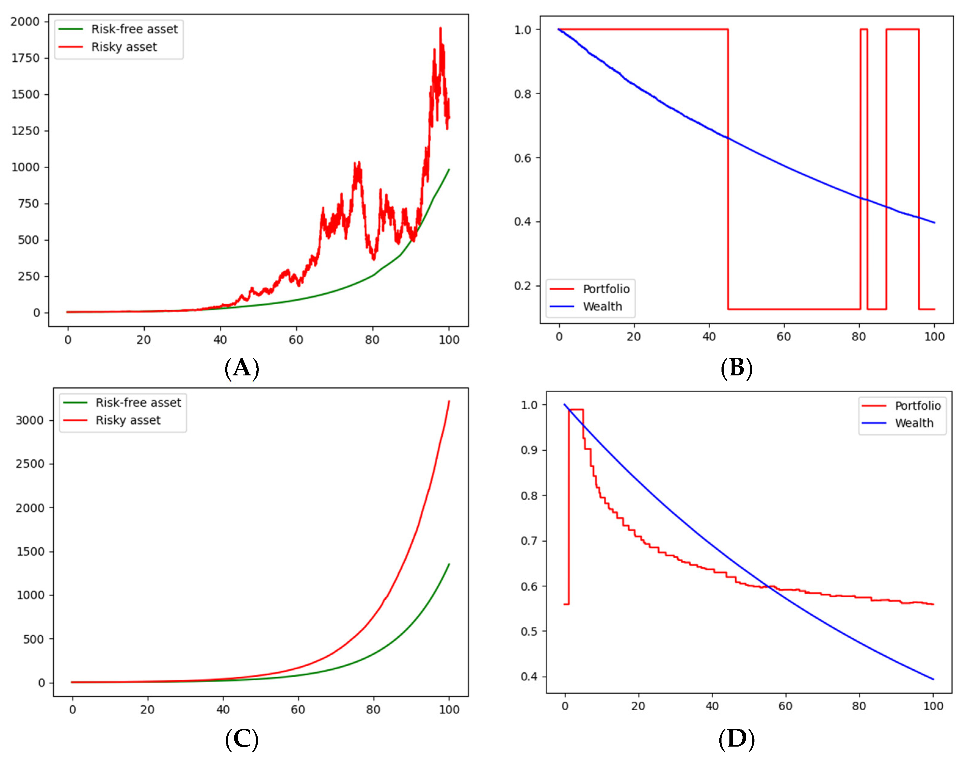
Figure 1A and
Figure 2A, show one realization for the price of the risky asset and one realization for the price of the risk-free asset (the bond). It can be seen that the risky-asset price follows a geometric Brownian motion with a changing trend (remaining the same volatility) and the bond price follows an exponential trend with a changing slope.
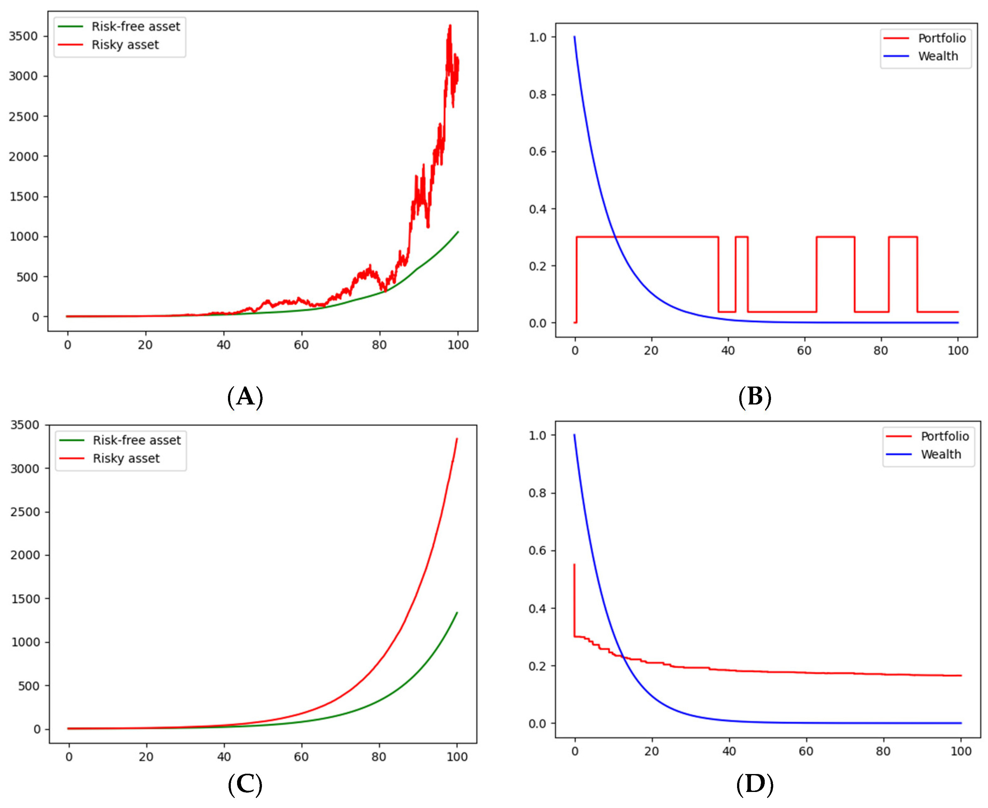
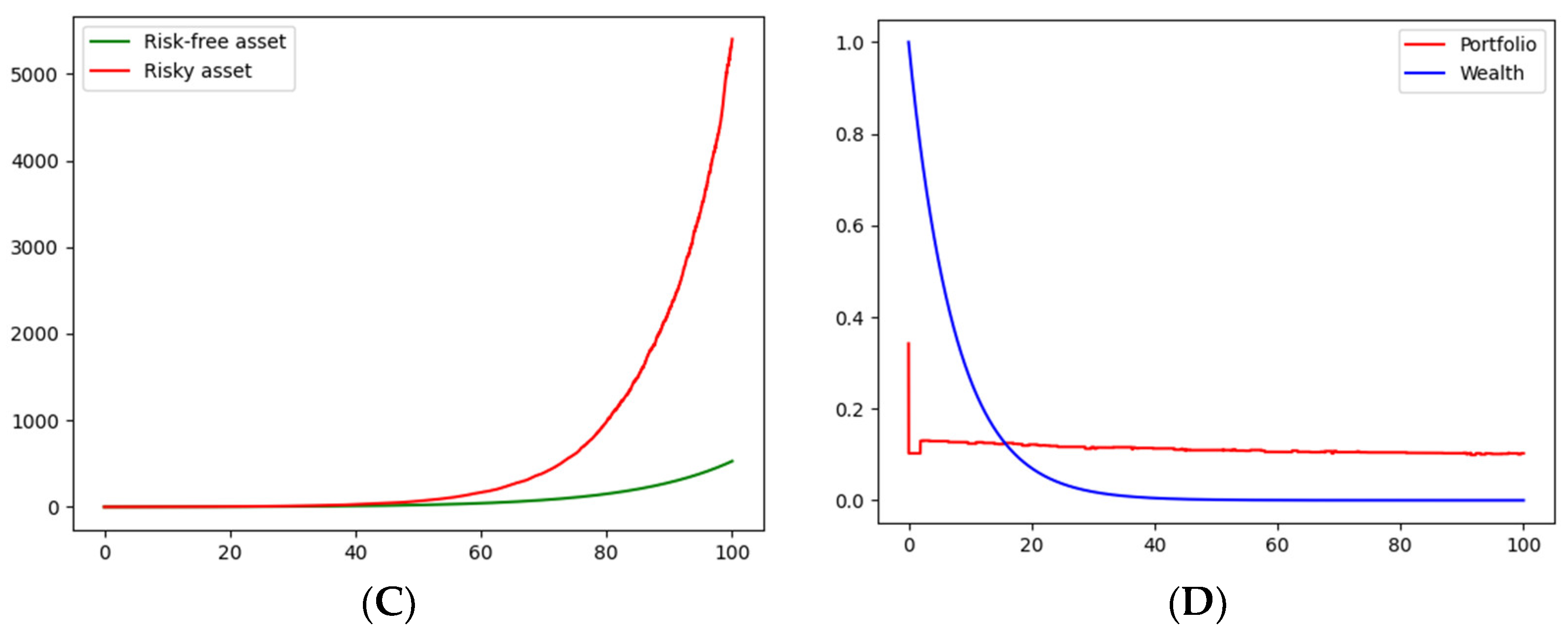
Figure 1C and
Figure 2C show an average of
realizations of the prices of the risky asset and the bond. In the cases of logarithmic and CRRA utility functions, one possible path for each of optimal decision variables, portfolio strategy, and consumption are presented, respectively, in
Figure 1B and
Figure 2B. Finally,
Figure 1D and
Figure 2D show the average path, with
simulations of the portfolio strategy and consumption, of logarithmic and CRRA utility functions, respectively. The values of the threshold,
k, were chosen, simply for illustrative purposes, as
k = 2 and
k′
= 1.5. Phyton 3.7 [
19] codes of the simulations are available on request.
In the simulation exercise, optimal portfolio decision seems, on average, more likely to be oriented to bonds, according to
Figure 1D and
Figure 2D. In addition, on average, we noticed convergence to a stable portfolio strategy in both the logarithmic and CRRA utility functions. Furthermore, the convergence speed seemed to be higher in the CRRA utility function. Moreover, since
in all simulations, the investor is anxious (or compulsive) about current consumption in such a way that what he/she receives in interest is not enough to compensate his/her consumption, so wealth will tend to zero in all cases. Finally, from (21) and (39), consumption is always proportional to wealth; thus, consumption tends to zero.
5.2. Second Scenario, Monotone Transition Probabilities
The second case considers a slightly different scenario from the previous one, with transition probabilities in terms of the ratio between
and
, though the states remain the same. We now establish the threshold,
for the ratio between
and
, in such a way that, at any instant, there exists a positive probability that increases as the mentioned ratio increases, allowing the second state to emerge in order to cut down the returns until the ratio is sufficiently small and the system goes back to “normal”. To accomplish this, we define the following transition matrix:
The value of the threshold was chosen simply for illustrative purposes as
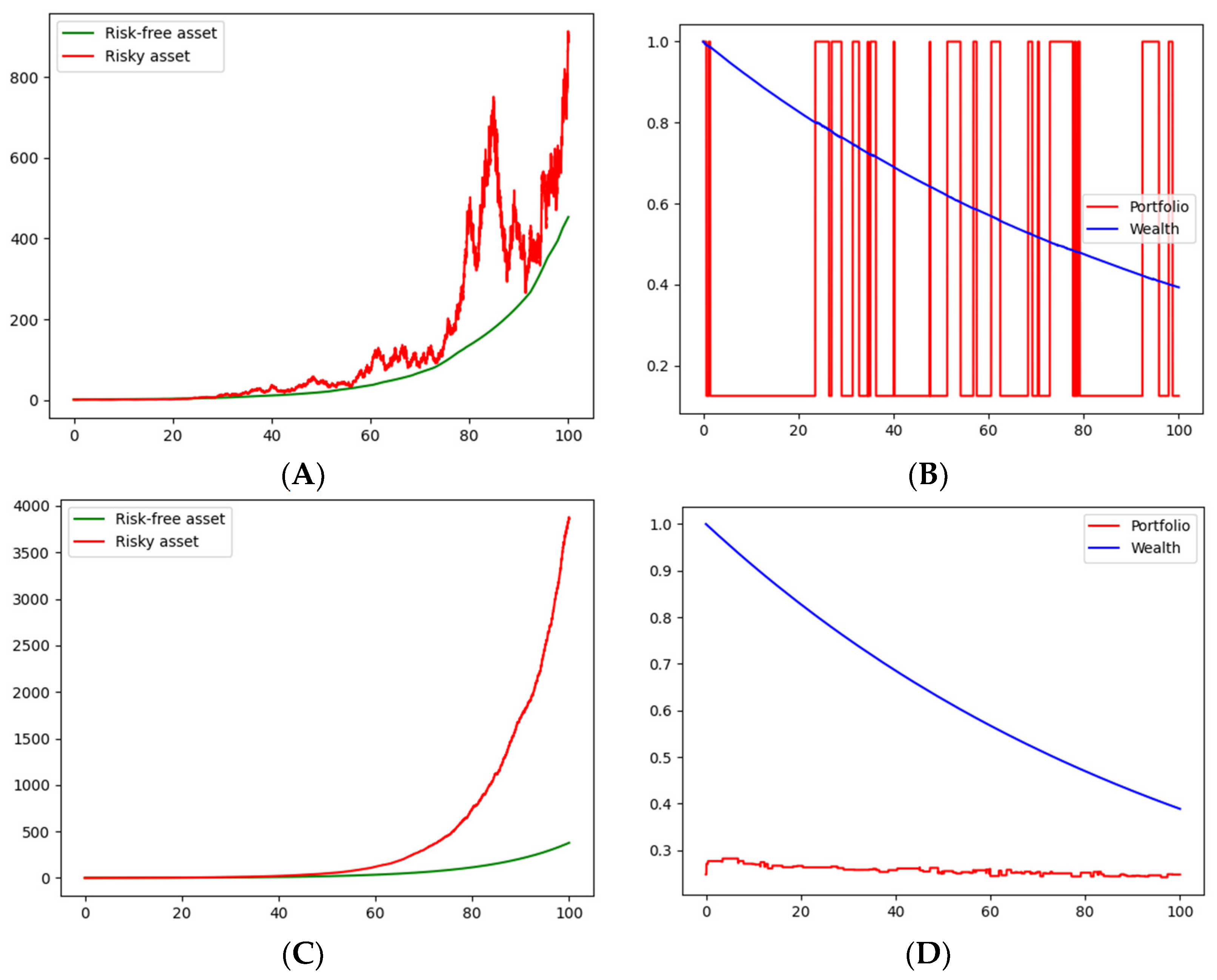
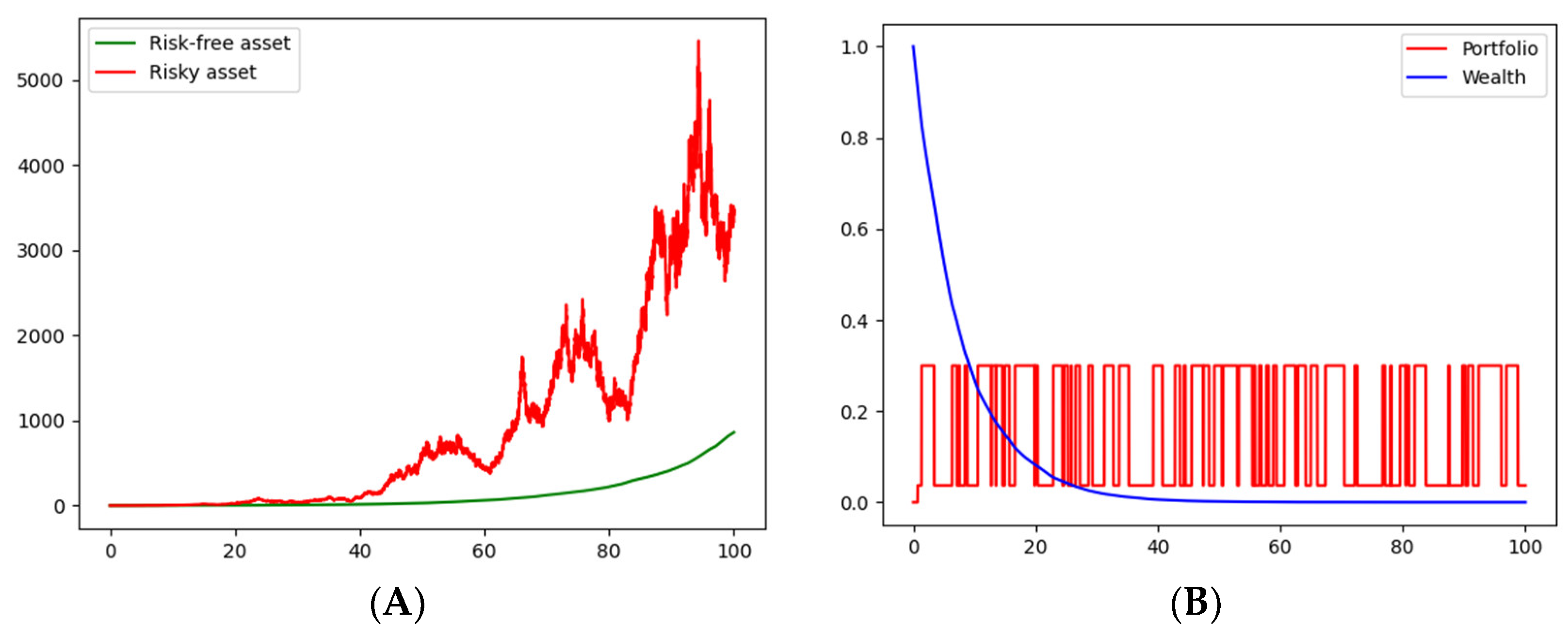
k = 2. As before,
Figure 3A and
Figure 4A show price realizations of the risky asset and the bond.
Figure 3C and
Figure 4C show the average of
price realizations of the risky asset and the bond. Possible paths of the optimal decision variables, in the cases of logarithmic and CRRA utility functions, are shown in
Figure 3B and
Figure 4B, respectively. Finally, the average path of the optimal decision variables, based on
simulations, are shown for logarithmic and CRRA utility functions, respectively, in
Figure 3D and
Figure 4D.
As seen in the first scenario, subsequent optimal portfolio decision seems more likely oriented to bonds, though now those appear more frequently (comparing
Figure 3B with
Figure 4B). After running several realizations, convergence to a stable strategy portfolio seems consistent for both the logarithmic and CRRA utility functions (
Figure 3D and
Figure 4D). Notice that the convergence speed, on average, seems to be higher than that of the first scenario.
6. Conclusions
This research found analytical solutions to the optimal-asset allocation problems of a rational consumer with logarithmic and CRRA utility functions, when the prices of the assets are modulated by a time-inhomogeneous Markov chain, with transition probabilities dependent on the stochastic dynamics of the risk asset (transition probabilities are themselves stochastic processes), which allowed for a deeper analysis of the decision-making process under uncertainty. Additionally, our proposal opens the possibility for improved interpretations of the parameters associated with specific regimes through transition probabilities dependent on asset prices.
It is worth mentioning that the goal of the simulations was to provide a basic, but meaningful, illustration with several scenarios to support the applicability of transition probabilities, when they themselves are stochastic processes. We developed an illustration of the theoretical results obtained for the Mexican case. Several scenarios were simulated by using the theoretical results found, demonstrating its potential as an analytical tool to effectively manage portfolio performance, based on an optimal rational allocation. Regarding the empirical results of all the simulations, convergence to a stable portfolio strategy was observed both for the logarithmic utility function and for CRRA. Furthermore, in all cases, on average, the optimal portfolio decision seems more bond-oriented, with wealth and consumption tending to zero.
The limitations identified in this investigation, such as the specific selection of a utility function, should be taken into account in future papers to search for more general analytical solutions. A promising direction is the use hyperbolic absolute-risk aversion (HARA), or negative exponential utility functions, to discover if the analytical solutions provide substantial differences compared to those found here, or if it is possible to identify general principles with all these utility functions useful for optimal portfolio allocation. In addition, more work should be performed to examine the sensitivity of the threshold . Finally, it is also very important to compare our proposal with alternative tools to model random events in future research.
Author Contributions
Conceptualization, data gathering, simulations, numerical tests, methodology, formal analysis, investigation, writing—original draft preparation, and writing—review and editing, B.V.-J., F.V.-M., O.V.D.l.T.-T. and J.Á.-G. All authors have read and agreed to the published version of the manuscript.
Funding
This publication was funded by the Consejería de Economía, Ciencia y Agenda Digital de la Junta de Extremadura and by the European Regional Development Fund of the European Union through the reference grant GR21161.
Institutional Review Board Statement
Not applicable.
Informed Consent Statement
Not applicable.
Data Availability Statement
Data are available upon request.
Acknowledgments
We, all authors, are very grateful to the four reviewers for carefully reading the document, and for the many useful and pertinent comments and suggestions that improved the final version of this work.
Conflicts of Interest
The authors declare no conflict of interest.
References
- Stockbridge, R.H. Portfolio optimization in markets having stochastic rates. In Stochastic Theory and Control; Pasik-Duncan, B., Ed.; Lecture Notes in Control and Information Sciences; Springer: Berlin/Heidelberg, Germany, 2002; Volume 280, pp. 447–458. [Google Scholar]
- Venegas-Martínez, F. Riesgos Financieros y Económicos; Productos Derivados y Decisiones Económicas bajo Incertidumbre; Cengage Learning: México, Mexico, 2008. [Google Scholar]
- Vallejo-Jiménez, B.; Venegas-Martínez, F. Optimal consumption and portfolio rules when the asset price is driven by a time-inhomogeneous Markov modulated fractional Brownian motion with multiple Poisson jumps. Econ. Bull. 2017, 37, 314–326. [Google Scholar]
- Carpinteyro, M.; Venegas-Martínez, F.; Aali-Bujari, A. Modeling precious metal returns through fractional jump-diffusion processes combined with Markov regime-switching stochastic volatility. Mathematics 2021, 9, 407. [Google Scholar] [CrossRef]
- Hamilton, J.D. A new approach to the economic analysis of nonstationary time series and the business cycle. Econometrica 1989, 57, 357–384. [Google Scholar] [CrossRef]
- Ding, K.; Cui, Z.; Wang, Y. A Markov chain approximation scheme for option pricing under skew diffusions. Quant. Financ. 2021, 21, 461–480. [Google Scholar] [CrossRef]
- Goel, A.; Mehra, A. A bivariate Markov modulated intensity model: Applications to insurance and credit risk modelling. Stochastics 2021, 93, 555–574. [Google Scholar] [CrossRef]
- Gapeev, P.V.; Rodosthenous, N. Optimal stopping games in models with various information flows. Stoch. Anal. Appl. 2021, 39, 1050–1094. [Google Scholar] [CrossRef]
- Gapeev, P.V. Discounted optimal stopping problems in continuous hidden Markov models. Stochastics 2022, 94, 335–364. [Google Scholar] [CrossRef]
- Maya, L.; Safra, B. Bond Risk Premia and Discount Rate Variation in Brazil. Available at SSRN 4047341. 2022. Available online: https://liviomaya.github.io/docs/research/2022-BondRiskPremiaDiscountRateVariationBrazil.pdf (accessed on 5 July 2022).
- Gluzberg, V.E.; Katz, Y.A. Impact of Transient Shocks to Productivity on Discounting of Long-Term Green Investments. Available at SSRN 4113486. 2022. Available online: https://papers.ssrn.com/sol3/papers.cfm?abstract_id=4113486 (accessed on 1 July 2022).
- Cousin, A.; Jiao, Y.; Robert, C.Y.; Zerbib, O.D. Optimal asset allocation subject to withdrawal risk and solvency constraints. Risks 2022, 10, 15. [Google Scholar] [CrossRef]
- Nukala, V.B.; Prasada Rao, S.S. Role of debt-to-equity ratio in project investment valuation, assessing risk and return in capital markets. Future Bus. J. 2021, 7, 13. [Google Scholar] [CrossRef]
- Pre-Criterios 2023, Secretaría de Hacienda y Crédito Público del Gobierno de México. 2022. Available online: https://www.finanzaspublicas.hacienda.gob.mx/work/models/Finanzas_Publicas/docs/paquete_economico/precgpe/precgpe_2023.pdf (accessed on 1 July 2022).
- Encuesta sobre las Expectativas de los Especialistas en Economía del Sector Privado: Mayo de 2022, 5 June 2022. Available online: https://www.banxico.org.mx/publicaciones-y-prensa/encuestas-sobre-las-expectativas-de-los-especialis/%7B293E2EAF-17C3-6D4E-F289-96A636F0435D%7D.pdf (accessed on 12 July 2022).
- Encuesta Citibanamex de Expectativas, 5 May 2022. Available online: https://www.banamex.com/sitios/analisis-financiero/pdf/Economia/NotaEncuestacitibanamex050522.pdf (accessed on 10 July 2022).
- Rivera-Hernández, E.C.; Venegas-Martínez, F. Análisis empírico de la tasa subjetiva de descuento para el consumidor mexicano. Eseconomía Rev. Estud. Econ. Tecnol. Soc. 2014, 9, 115–132. Available online: https://econpapers.repec.org/article/ipnesecon/v_3aix_3ay_3a2014_3ai_3a40_3ap_3a115-132.htm (accessed on 1 July 2022).
- Conine, T.E.; Michael, B.; McDonald, M.B.; Tamarkin, M. Estimation of relative risk aversion across time. Appl. Econ. 2017, 49, 2117–2124. [Google Scholar] [CrossRef]
- Phyton 3.7. Gzipped Source Tarball, XZ Compressed Source Tarball. Available online: https://www.python.org (accessed on 13 July 2022).
Figure 1.
First scenario, logarithmic utility, , , and . Natural momentum (, , ) vs. inferred momentum (, , , with . (A) Price realization, (B) Portfolio strategy, (C) Average of price realizations, and (D) Average of portfolio strategies. Authors’ own elaboration.
Figure 1.
First scenario, logarithmic utility, , , and . Natural momentum (, , ) vs. inferred momentum (, , , with . (A) Price realization, (B) Portfolio strategy, (C) Average of price realizations, and (D) Average of portfolio strategies. Authors’ own elaboration.
Figure 2.
First scenario, CRRA utility, , Natural momentum , , vs. inferred momentum , , , with , and . (A) Price realization, (B) Portfolio strategy, (C) Average of price realizations, and (D) Average of portfolio strategies. Authors’ own elaboration.
Figure 2.
First scenario, CRRA utility, , Natural momentum , , vs. inferred momentum , , , with , and . (A) Price realization, (B) Portfolio strategy, (C) Average of price realizations, and (D) Average of portfolio strategies. Authors’ own elaboration.
Figure 3.
Second scenario, logarithmic utility, Natural momentum (, , vs. inferred momentum (, , , with . (A) Price realization, (B) Portfolio strategy, (C) Average of price realizations, and (D) Average of portfolio strategies. Authors’ own elaboration.
Figure 3.
Second scenario, logarithmic utility, Natural momentum (, , vs. inferred momentum (, , , with . (A) Price realization, (B) Portfolio strategy, (C) Average of price realizations, and (D) Average of portfolio strategies. Authors’ own elaboration.
Figure 4.
Second scenario, logarithmic utility, Natural momentum , , vs. inferred momentum , , , with , and . (A) Price realization, (B) Portfolio strategy, (C) Average of price realizations, and (D) Average of portfolio strategies. Authors’ own elaboration.
Figure 4.
Second scenario, logarithmic utility, Natural momentum , , vs. inferred momentum , , , with , and . (A) Price realization, (B) Portfolio strategy, (C) Average of price realizations, and (D) Average of portfolio strategies. Authors’ own elaboration.
| Publisher’s Note: MDPI stays neutral with regard to jurisdictional claims in published maps and institutional affiliations. |
© 2022 by the authors. Licensee MDPI, Basel, Switzerland. This article is an open access article distributed under the terms and conditions of the Creative Commons Attribution (CC BY) license (https://creativecommons.org/licenses/by/4.0/).


 ,
, 


