1. Introduction
Credit risk is a risk that rises from the possibility of a borrower failing to repay a loan or required payments, or meeting its contractual obligations, and is determined by a borrower’s ability to repay a loan according to its original terms [
1]. Credit rating is a quantified assessment of credit risk and is therefore used to evaluate the credit risk of an individual, corporation, or state [
2]. It can be determined and calculated by any entity using the internal and publicly available data and models, or, more commonly, by a credit rating agency [
3]. The credit rating agency specializes in calculating credit ratings using its internal models and both publicly available and non-public information. A sovereign credit rating is a credit rating assigned to a country. Due to a large amount of available information and the importance and implications that a sovereign credit rating has on a country due to quantifying its financial, industrial, social, and political stability [
4], a sovereign credit rating is usually determined by the trustworthy credit rating agencies which are overseen and regulated [
5]. The three biggest agencies that control nearly 95% of the credit rating business are Moody’s Investors Service (Moody’s), Standard and Poor’s (S&P), and Fitch Ratings (Fitch).
One of the major concerns about credit ratings is the lack of transparent models used in order to determine the ratings. In today’s financial world where most of the basic instruments and derivatives such as futures, forwards, swaps, and options have explicit and verified pricing models, it is a considerable drawback not to have a similar publicly available transparent and closed-form solution for credit ratings. Therefore, this can lead to a violation of a non-arbitrage principle and cause serious economic issues for a country and its debtors and creditors if its rating is incorrectly determined. The non-transparency of the models used by credit rating agencies has resulted in many internally developed models for credit rating prediction by both other participants in the market as well as researchers for academic purposes.
Custom credit rating approaches and models can be utilized for the validation and deeper understanding of the models implemented by credit rating agencies [
3,
6]. Even though these agencies are supervised [
5,
7], it is inadvisable that the only publicly recognized credit rating models are essentially black boxes. Having several independently developed models reduces the potential information incompleteness and ensures a no-arbitrage principle in the credit risk market. Further, the benchmarks used for the training of the custom models are mostly taken from the published reports of the credit rating agencies [
8]. Therefore, the obtained results emulate ratings of the credit rating agencies and usually cannot be as precise as theirs. On the other hand, the trained models can be used for forecasting ratings of the companies and entities not listed on the stock exchange [
9].
In the 1990s, the majority of custom-made credit rating approaches were based on traditional financial modeling and econometrics. The first methods presented in the literature utilized either linear [
10] or multiple regression [
11], followed by models based on ordered logistics and probit [
12,
13,
14] regression, as well as their generalized version G-logit [
15]. These models were also compared against each other [
16], as well as against other methods, such as case-based reasoning [
17] and partially ordered set [
18], where no best model could be clearly determined. Even though these models were easy to implement and understand, some of the most common drawbacks of these models are underfitting, inability to fully capture the nonlinear nature of the problem, and the assumptions necessary for methods to apply to the desired problems, which then led to the more frequent application of the machine learning (ML) and computation intelligence (CI) methods. Given the complexity of the problem [
10,
13,
19], the fact that models used by credit rating agencies are non-transparent, and the rising popularity of the ML and CI over the last decade, these methodologies were a natural choice for deriving custom forecasting models that use publicly available microeconomic and macroeconomic indicators [
11,
20,
21,
22]. Nowadays, the majority of the custom-made models for credit rating forecasting are based on ML and CI techniques or as a hybridization of several methods. Most of the models built this way are based on an input-output logic, meaning that the model is provided with the chosen inputs and desired outputs, and it is expected to form a relation between the two in the training process in order to later apply that relation on newly provided inputs to predict the desired outcome. The model construction can therefore be split into several steps, for example, choosing the financial or economic dataset and time frame, choosing the appropriate forecasting technique, model training, and model testing. The main idea of using the machine learning techniques for credit rating analysis and forecasting, such as neural networks (NN), is used both solely [
8,
23,
24] and in hybrid models with a genetic algorithm [
25] and fuzzy logic [
26,
27]. There were also attempts on using unconventional NN models for credit rating forecasting such as emotional neural networks [
28] and networks with unusual learning schemes [
29]. Other ML techniques for credit rating forecasting include support vector machines (SVM) [
30,
31,
32], genetic algorithms [
33,
34,
35,
36], and fuzzy logic [
37,
38,
39]; all of these methods tend to improve the forecasting obtained by classic econometric methods. NNs are not only used for credit rating forecasting, but also in close fields, such as forecasting credit risk [
40] and credit rating for bonds [
41]. Each of the techniques mentioned has some disadvantages, e.g., the inability to interpret results for NNs, computational efficiency for genetic algorithms, the need for vast knowledge and expertise in order to use fuzzy logic to deal with a certain problem, etc. Therefore, ML techniques that can be used solely as predictors, such as NNs and support vector machines, which are later used in this paper as benchmark models, are combined with fuzzy logic and genetic algorithms in order to eliminate downsides and create superior hybrid models. Further, the drawback of several models proposed in the literature is that there are no clear conclusions whether they are better than their comparison models, as well as using too short data time frames with a time span of only several years, which makes the predicted results questionable in any other time period. Therefore, when the new model is introduced, it is vital that it clearly outperforms the target models in a longer time frame in order to claim its efficiency and performance improvement compared to the benchmark models.
In this paper, we propose the usage of Differential Evolution (DE) and interpolative Boolean algebra (IBA) to extract an aggregation function, logical by its nature, for forecasting sovereign credit ratings. DE is a biological-inspired optimization heuristic from a family of evolutionary computational algorithms [
42]. In our approach, DE is used to detect patterns, interactions, and co-dependencies in historical data as a search algorithm. On the other hand, IBA is a consistent-valued realization of Boolean algebra [
43] which preserves all the laws of the BA. Therefore, IBA provides a real-valued logic-based framework that is consistent with Boolean axioms. In the IBA-DE approach, logical and pseudo-logical IBA functions are employed as an aggregation function and further used for prediction. These functions have clear-cut meaning and they are easy to understand and analyze. Thus, the proposed approach is transparent and allows deeper insight into the observed problem. This approach can be divided into three main steps: selecting appropriate indicators and their transformation using IBA for inputs suitable for the DE algorithm; using the DE algorithm on the input data in order to obtain optimal IBA structure vectors; and applying IBA logical aggregation on the inputs and structure vectors to obtain the forecasted credit ratings.
This paper extends and continues the research started in [
44], where the idea of using the DE algorithm for the optimization of a prediction model structure in the IBA framework is presented for the first time. In this paper, the IBA-DE algorithm is elaborated on in detail and used for sovereign credit rating prediction. The model is a pseudo-logical function that uses publicly available macroeconomic indicators to predict sovereign credit ratings. Compared to the research presented in [
44], where only the financial inputs have been used, the inputs used in this paper are extended to encompass the industrial and social country aspects. The function which is obtained as a model output is easily analyzed and interpretable due to the fuzzy gradation of its elements. Additionally, the performance of the proposed approach exceeds back-propagation NNs.
The paper is organized in the following manner. In
Section 2, we give a brief overview of the theoretical background, i.e., the two main methodologies used in the hybrid model, the DE algorithm and the IBA logical framework. The basic idea behind the IBA-DE approach and the main steps of the algorithms are presented in
Section 3.
Section 4 is devoted to the application of the IBA-DE approach to sovereign credit rating prediction. We present the two model realizations, along with their inputs, parameters, benefits, and limitations. The testing results are presented in
Section 5, together with a parameter optimization process and a detailed interpretation of the results. The models’ performances are further compared with the neural networks. Finally, in
Section 6, we outline the main conclusions and give ideas regarding model improvements and future work.
3. IBA-DE Approach
In this section, we introduce the IBA-DE hybrid approach. It is a logic-based ML approach that utilizes the extensive modeling benefits of the IBA framework and its presentation potential.
There have been a few attempts to hybridize the IBA framework with some optimization heuristic in order to learn a LA function from the data. In fact, a variable neighborhood search [
56] and genetic algorithm [
57] were used to optimize binary values of the IBA structure vector on different datasets, showing promising results. However, the full potential of the IBA framework is not utilized in these cases, i.e., the final model is a simple LA and not a pseudo-LA function.
In an IBA-DE approach, the aim is to obtain a structured vector of the pseudo-LA function as an output aggregation function that is more general compared to LA. IBA-DE is the first attempt to perform optimization of the structure vectors in the continuous space. The main idea is to use IBA to transform raw data points into suitable inputs for the DE algorithm, and then to use DE to find an optimal solution for the observed problem. Since the final model is a pseudo-LA function, IBA-DE may be considered a white-box model, i.e., it can be easily analyzed and interpreted.
Herein, we present the step-by-step implementation details and give pseudo code for non-vanilla parts of the hybrid algorithm.
3.1. The Main Steps of the IBA-DE Algorithm
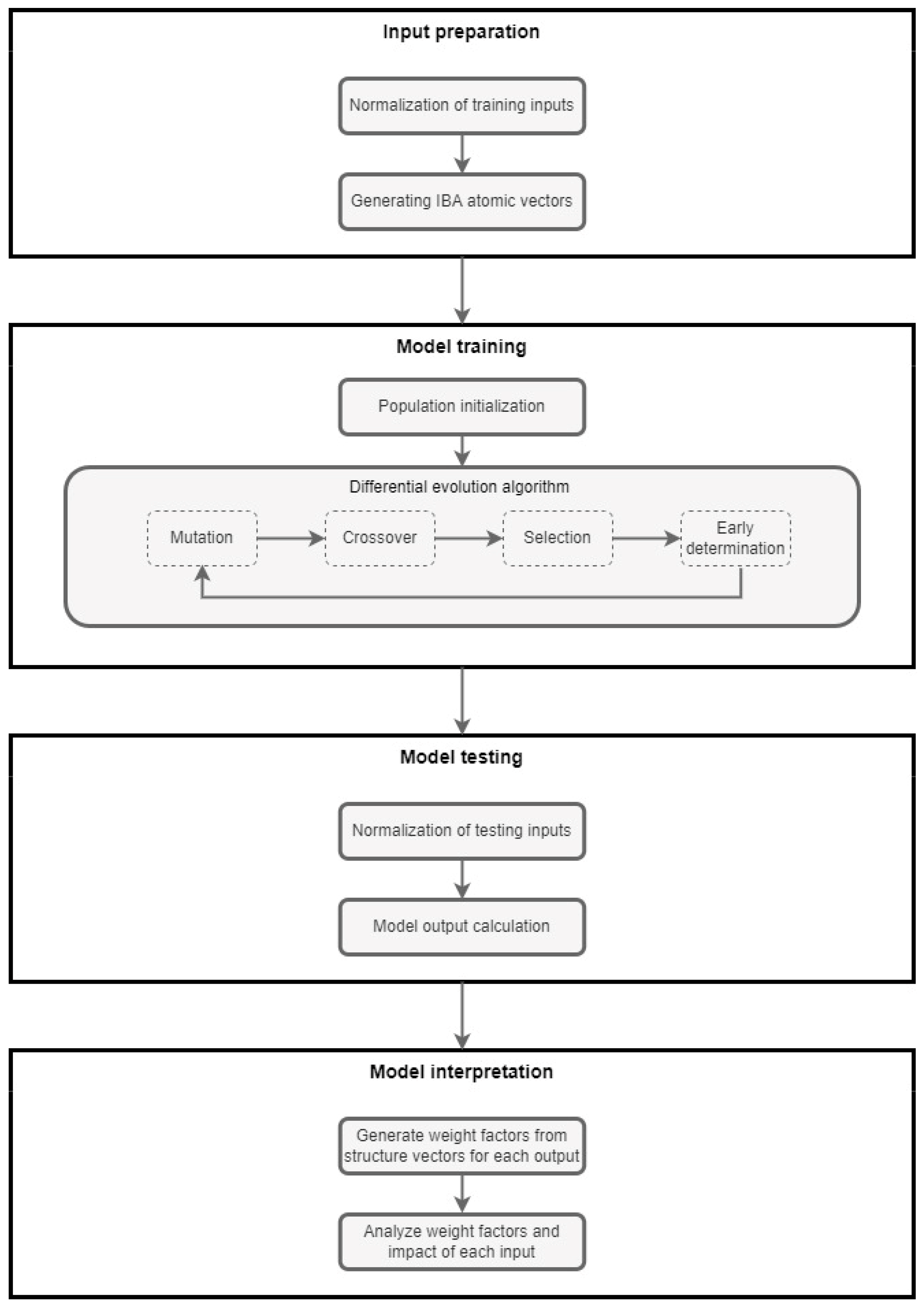
The IBA-DE approach consists of four main steps:
Input preparation;
Model training;
Model testing;
Model interpretation.
A more detailed presentation of the algorithm is given in
Figure 1.
Input preparation: The first step in the IBA-DE approach refers to the input preparation, and it consists of the normalization of training inputs and generating IBA atomic vectors. Since we are modeling and inferring in the IBA framework, all elements of input vectors must be valued on an
interval. Any normalization function can be used for this purpose. Still, classical min-max normalization along with some methods for handling outliers is a common choice. Data preparation for optimization is performed by generating and valuing IBA atomic vectors. Let
be the
g-dimensional input vector and let
A be the
d-dimensional atomic vector. Each element of the input vector is an IBA attribute, while each element of the atomic vector is an IBA atom. Every element of the atomic vector represents one distinctive combination of attributes. It is represented as a product,
, where
and
is a normalized value of an attribute. In
Section 2.1, it was stated that the relationship between the dimensions of input and the atomic vector is
, i.e., the number of atomic elements will exponentially increase with the increasing number of inputs. For instance, an atomic vector created from the two-dimensional input vector consists of four elements and it is shown in Equation (4).
Therefore, for the dataset of
m g-dimensional input vectors, the result of IBA transformation is a dataset of
m d-dimensional atomic vectors. This is the input in the DE algorithm where an optimization process will take place. The pseudo-code for generating atomic vectors from the input vectors is given in
Appendix A.
Model training: After the inputs are prepared in a manner suitable for DE optimization, the model training step may begin. The main goal of this phase is to obtain the optimal structure vector which will minimize the objective function, e.g., mean squared error (MSE) of prediction. In our case, elements of a structured vector are in the unit interval. Therefore, the pseudo-logical aggregation function [
51] is obtained as a final output. This function is easy to interpret since it is basically a weighted sum of several logical functions. The DE algorithm used for optimization is the basic one with the steps described in
Section 2.1. In addition to a typical stopping condition defined as a maximal number of iterations, we have included an early stopping, a standard machine learning mechanism to avoid model overfitting. Three DE control parameters may be considered as hyper-parameters important for model training:
,
, and the population size. Their values should be assessed during the training phase in order to maximize the potential of the IBA-DE approach.
Model testing: The trained model is assessed and utilized in the model testing step of IBA-DE. A product of the atomic vector of an observed instance and the transposed optimal structure vector are the numerical values that are being forecasted, as explained in
Section 3.2. All attributes should be scaled to a unit interval using the same normalization function as in the model training step. The final prediction may be validated by comparing the benchmarks, or re-evaluated if some input data changes in time.
Model interpretation: The final phase of the IBA-DE approach is the model interpretation step. The output of the DE algorithm is an optimal structure vector whose atoms are used to create the appropriate weight factors for each of the inputs. The weights show the impact of every input, compared to all other inputs, on the forecasted credit ratings. With this information, all inputs can be ranked and the ones with the lowest impact discarded or replaced with new ones. The model is therefore not only predicting the credit ratings but also giving the information necessary for further decision-making, and, therefore, cannot be considered a black box but rather an instrument that can be used not only for forecasting but also for the interpretation of the obtained results.
3.2. Benefits and Limitations
The IBA-DE hybrid algorithm is part of a general approach to utilize the IBA framework in a machine learning context. The final model is easy-to-understand, transparent, and universal since it utilizes a pseudo-LA function. Thus, the range of possible applications is very wide, i.e., any small-scale forecasting problem.
In our approach, the basic DE algorithm [
42] is used, rather than some of its modifications. Many proposed hybrid DE algorithms are not easily reproduced due to various reasons. Even though the pseudo-code is provided for the majority of hybrid algorithms, the source code is not always available. Some algorithms are also created using overly complicated premises, where hybrid models are enhanced with additional techniques such as Adaptive Pursuit and Probability Matching [
58]. This makes these models a bit difficult to understand and implement. Finally, many of the mentioned algorithms have not been tested on real-world problems but were rather made in order to improve general DE premises and/or to test them against other hybrid models in various yearly CEC DE competitions where different problems and hypothetical objective functions are defined [
59,
60]. These are all the reasons for not using any hybrid DE models which update control parameters and strategies during the iteration process.
The main drawback of the IBA approach is that it is not well suited for high-dimensional inputs due to the exponential growth of atomic vector size and therefore makes DE optimization slower. However, the trade-off for using IBA and the LA in the process is the interpretability of the forecasted results. Many machine learning techniques, such as NNs, are black-boxes and their results are not easily explainable. Thus, the interpretation of their results is a serious problem in many practical situations. This is evident in areas such as finance where a decision must be understood and explained before any action is taken. Therefore, the exponential increase in complexity with the linear increase in the inputs is a cost willingly paid for the interpretability of the end results and seeing how much each of the inputs influences the output. In addition, with the many dimension reduction methodologies, such as principal component analysis or different kinds of regression, it is possible to reduce the number of inputs and allow the IBA-DE model to provide results without losing valuable information in the process.
4. Forecasting Sovereign Credit Ratings with the IBA-DE Approach
In this section, we present the application of the IBA-DE approach for sovereign credit rating prediction. The approach was first used for credit rating prediction in [
44]. However, the inputs used were from a very narrow domain and many aspects of the economy were not considered. Further, the parameters of the DE algorithm were obtained empirically, without sensitivity analysis or testing different combinations of parameters. In this paper, we extended the input space to include a broader domain of economic factors and also to take into consideration historical credit ratings. The latter is especially important for improving forecasting performance since the changes in credit ratings are considered rare events.
In the first part of this section, we discuss the input space and give an overview of the input variables. Input space was divided into two categories: historical credit ratings and macroeconomic factors. Three groups of macroeconomic factors were used in this study to take into account different aspects of a country’s economic strength and to discover those with the highest influence on credit ratings.
In the second part, we present two different forecasting approaches:
A single-aspect approach where different groups of macroeconomic factors (stability, activity, and social) are used separately to forecast sovereign credit ratings;
A multi-aspect approach that uses all groups of input variables to include a broader perspective in the prediction model;
These forecasting approaches were used to run two types of forecasts: with and without historical credit ratings. First, our goal was to run our models only with macroeconomic inputs to understand the influence of different factors on sovereign credit ratings. Second, we replaced the worst performing factor within our model with the historical credit ratings and ran the model again (train and test).
4.1. Inputs
Most studies that dealt with the credit rating determinants show that financial and economic indicators have the highest impact on the credit ratings [
13,
61]. Some of the factors which are highly correlated with the sovereign credit ratings are GNP, GDP, GNI, inflation, government income and debt, unemployment, and default history [
13,
62,
63,
64]. Indicators are usually selected based on their correlation to credit ratings data, or derived using some method such as a principal component analysis [
65]. Some studies show that financial and economic factors are not the only ones to influence credit ratings [
13,
66]. Consequentially, unorthodox factors such as monetary policy credibility, government debt structure, financial sector depth, foreign currency dependence, and others are included in the recent studies [
19]. In most papers, authors investigate how individual factors influence sovereign credit ratings, but do not consider the influence of groups of factors.
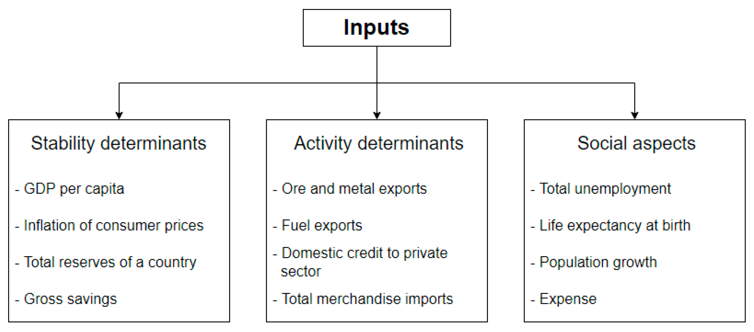
In this study, we used two types of inputs for our IBA-DE model: macroeconomic factors and historical credit rating. Macroeconomic factors are grouped into three groups: stability, activity, and social. Our idea was to enable our model’s broader perspective so that no individual group of factors would have a dominant influence on a credit rating. Each group consists of four indicators (
Figure 2). Indicators were carefully selected based on two criteria: availability of data and their ability to outline a broader view of the aspect that characterizes the group. We have a limited number of inputs per group of four to keep the model as simple as possible and to avoid exponential growth in the size of IBA’s atomic vector size (explained in
Section 3.2).
The first group of indicators represent economic stability determinants. These factors are frequently used by researchers and are proven to be the ones to impact a country’s credit ratings the most. In this paper, we have used the following indicators: GDP per capita, as one of the best indicators of a country’s economic strength and development; inflation of consumer prices, to include a measure of the quality of life of an average household; total reserves of a country, including gold, to represent the country’s ability to face unpredicted events and crises; and gross savings, as an indicator of country’s investment strength.
The second group of indicators represents economic activity determinants. When choosing these variables, our idea was to take into consideration the export, import, and credit activity of a country. The following indicators were used: ore and metal exports and fuel exports, as an indicator of a country’s strategic independence on energy and raw materials, due to increasing prices caused by supply chain bottlenecks, high inflation, and the latest geopolitical changes; domestic credit given to the private sector as an indicator of the country’s willingness to support its private sector; total merchandise imports, as an indicator of country’s dependence on import of goods.
The third group of factors provides an overview of the social aspects of a country’s economy. The following four indicators were selected as measures of a country’s social policies and overall quality of life: total unemployment, which shows how effectively a country deals with unemployment; life expectancy at birth, as one of the best indicators of the quality of life; population growth, which is an indicator of the potential for future economic growth; and expense, measuring the government’s spending.
All the above-mentioned input data were obtained from the World Bank (
data.worldbank.org (accessed on 30 September 2020)). Our dataset covers 83 countries (listed in
Appendix B) and 19 years of data, from 2000 to 2018. The countries were selected based on the availability of indicator data, to achieve as much variety as possible regarding the location and population size. Even so, there were some gaps (missing data) in the dataset due to such a long time range. These missing points are filled using linear interpolation and flat extrapolation.
4.2. Output
Sovereign credit ratings data were obtained from the Fitch Ratings (
https://countryeconomy.com/ratings (accessed on 30 September 2020)) because they are publicly available for the countries used in this study and for a time span of 19 years. Given the similarity of the published ratings between the three top credit rating agencies, no information is lost by choosing any one of them. Fitch’s ratings are divided into categories (
Table 1). We transferred credit rating categories into representative numerical values from the [0, 100] interval. The reason for using a numerical rather than a categorical variable was to increase precision and enable fuzzification of credit ratings. Using numerical values will cause this classification problem to transform into a forecasting problem. The representative values are assigned in a way to maximize the distance between the ratings within a category, and therefore to maximize the forecasting accuracy. Further, the fuzzification of credit ratings is done by adding representative intervals around the representative values (
Table 1).
In the IBA-DE approach, credit ratings are forecasted as numerical values which are then sorted into numerical intervals and finally converted back to the appropriate credit rating categories. In addition, numerical outputs could be used for confidence interval extraction, based on the absolute difference between the forecasted values and the center of the credit rating’s representative intervals.
4.3. Forecasting Models
Using the hybrid IBA-DE approach, we built two types of forecasting models. First, we used three groups of input data separately, each group representing a different aspect of a country’s economic strength, to make separate (specialized) predictions of sovereign credit ratings. Second, we used all three groups of input data together to make broader-perspective predictions of sovereign credit ratings that take into account multiple aspects of the country’s economic strength.
4.3.1. Single-Aspect Model
Single-aspect models use only one group of input factors to predict sovereign credit ratings. They are meant for two reasons:
To investigate whether specific aspects of a country’s economic strength could produce satisfactory predictions and therefore reduce input space or substitute some group(s) of factors instead;
To provide the aggregated (multi-aspect) model with optimal inputs.
Input data were used to create IBA atomic vectors which are further used as input variables for the DE algorithm. Then, the DE algorithm optimizes the structure vector to minimize the objective function which is the mean square difference (MSE) between credit rating forecasts and targeted (real) numerical values. The initial population of structure vectors was generated in a random way. Credit rating forecasts,
, were obtained from quadruplets of input data by multiplying the corresponding atomic vector,
, with the transposed optimal structure vector,
, as shown in the Equation (5):
4.3.2. Multi-Aspect Model
The multi-aspect model represents an aggregated approach for credit rating prediction which considers different aspects of a country’s economic strength. This model uses the previously explained single-aspect models as components, more precisely, their optimal structure vectors. Therefore, to run this model, one must first run three separated (single-aspect) models, one for each group of input factors. The obtained vectors of the structure are linearly aggregated in a weighted sum to obtain multi-aspect predictions. The credit ratings are forecasted as shown in Equation (6):
where
,
and
represent weightings for single-aspect structure vectors. The objective function is the same as for the single-aspect models, while the optimization is now done to obtain the optimal vector of weights, rather than the optimal structure vector.
5. Experiment and Results
In this section, we test the two models proposed in
Section 4.3. The models are tested against the benchmark ratings obtained from the Fitch credit rating agency. First, we describe the dataset used for this study. Further, we deal with parameter optimization and model training: analyzing the impact of the DE control parameters on the training process and obtaining optimal structure vectors on the training set. After model training, we aim to investigate the resulting IBA structure vectors to provide a deeper insight into the significance of inputs as well as their co-dependencies. Finally, the forecasting performance of IBA-DE models is compared with NNs, given that NNs are one the most used machine learning techniques for credit rating prediction.
As explained earlier, our models use three groups of macroeconomic inputs to take into account three different aspects of a country’s economic strength: stability, activity, and social aspect. Indicator values were calculated on an annual basis and normalized on the unit interval.
5.1. Data
Our dataset consists of 19 years of macroeconomic data for 83 world countries. There are three groups of input data with each group consisting of four macroeconomic indicators–in total, 4731 quadruplets of input data or 18,924 input observations. On the other side, there is only 1 output variable with 1577 observations.
We split the dataset into two subsets: training and testing. We used 17 years of data (2000–2016) to train our models, which counts as 16,932 input and 1411 output observations. The last two years (2017–2018) were used for testing purposes, yielding 1992 input and 166 output observations.
Therefore, we split our dataset on training and test sets using a higher than usual 90–10 split ratio. This could create a risk of overfitting for NNs, which are used as benchmark techniques for the proposed IBA-DE models. However, the risk of overfitting is relatively small due to slow changes in credit ratings over the years.
5.2. Hyper-Parameter Optimization and Training
As usual in machine learning, the model selection is performed in two phases. Bearing in mind that the IBA part of the IBA-DE approach is non-parametric, only the DE control parameter: , , and the population size are considered as the model’s hyper-parameters. In the first phase, we aimed to assess the training convergence speed depending on the values of hyper-parameters and, subsequently, to determine their impact on the model output. The second phase was devoted to an appropriate training procedure in order to obtain the optimal structure vectors, avoiding model overfitting and biased predictions.
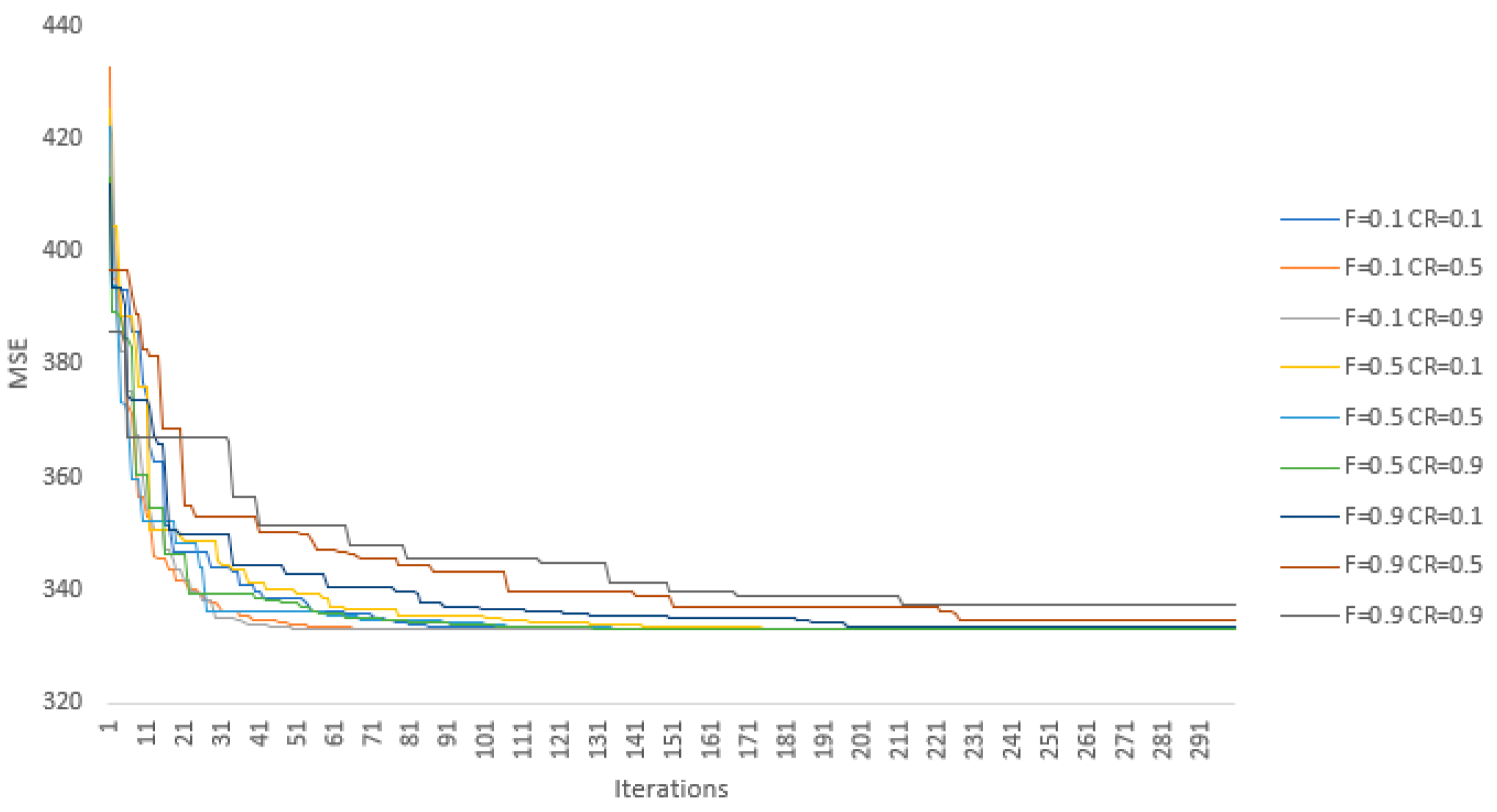
In the first phase of model selection, we employed a grid search by varying values of the control parameters and between 0.1 and 0.9 with a 0.1 step. In addition, three values of the population size are considered: 10, 100, and 1000. Thusly, we performed optimizations, i.e., model training processes, for each of three input sets: stability, activity, and social. This procedure was conducted on the training set, while the stopping criterion was defined as the fixed number of iterations, i.e., 300, in order to observe the model convergence over a longer period of time. Additional termination conditions are if the absolute difference between 100 consecutive objective functions is less than , or if the objective function reaches 0. Due to the stochastic nature of DE, five simulations were conducted per combination of the control parameters with random starting points.
The DE algorithm has reached the same optimal solution for each parameter set in 97.5% of cases. In addition, the convergence paths with respect to the MSE presented in
Figure 3 and
Figure 4 are reasonably similar. However, in the other 2.5% cases, the algorithm became stuck in local minima that are rather close to the best result. Still, these results emphasize that the values of hyper-parameters
and
are not crucial for the final results of the optimization. This can be seen in
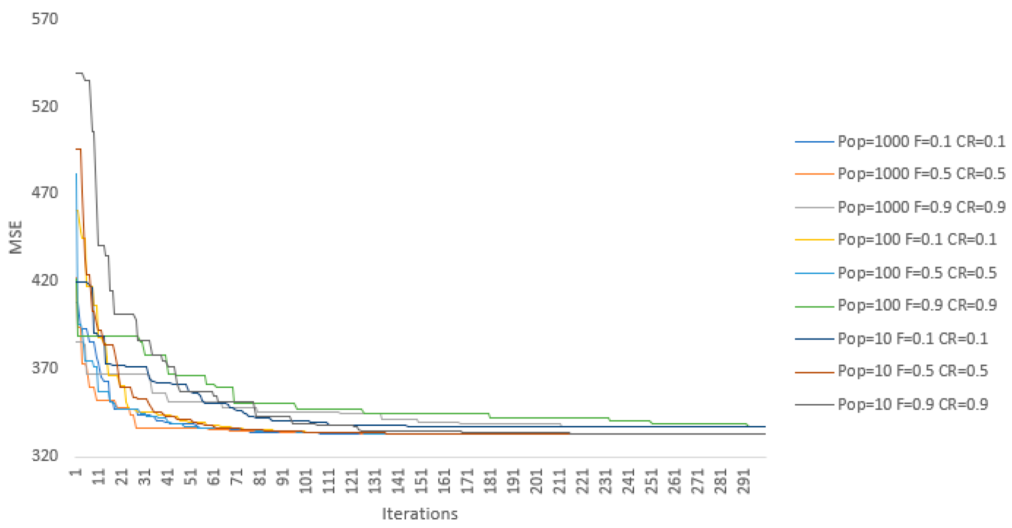
Figure 3, where no significant co-dependency can be seen between parameters’ values and model behavior. There is also no significant difference between model results for the population sizes of 100 and 1000, even though the latter converges a bit faster on average but not fast enough to justify a 10 times larger population size (see
Figure 4). The model with a population size of 10 has slightly worse results, although for some control parameter combinations the model performs as well as the ones with higher population sizes. However, when inputs are amended with the historical credit ratings, the model with a population size of 10 achieves significantly worse results compared to the models using population sizes of 100 and 1000. Therefore, in our case, the recommendation is to use a medium population size when one of the inputs has a strong co-dependency with the output. Otherwise, the model can be defined as non-parametric. Finally, the results of the chaining forward cross-validation have supported this conclusion.
Therefore, we performed a model training with the following hyper-parameters values:
,
, and the population size equal to 100. We employed an early stop stopping criterion in order to avoid model overfitting. The best results on the training data set, including the objective function values and the number of iterations necessary to achieve them, are presented in
Table 2.
As can be seen from the table, the multi-aspect model performs slightly better than the single-aspect models, which is to be expected. The model using solely the activity inputs performs better than the models using stability and social inputs, while when the historical credit ratings are added, the differences between the models are negligible due to the high impact of the historical time series.
Finally, the main output of the optimization process is the IBA structure vector which is then used in generating forecasted credit ratings.
5.3. Test Results and Interpretation
In financial decision making, the transparency of models and interpretation of the data often play a crucial role. Sometimes, the most accurate models are not applied if they are not transparent or too complex for understanding. When introducing the IBA-DE approach we addressed this issue. Namely, IBA-DE is considered a white-box model, since its structure vector can be quickly analyzed to determine the significance of individual input factors and their co-dependencies [
67]. The IBA structure vector consists of weights representing atoms’ importance in the model–the higher the weights, the higher the influence on predictions. In this section, we presented and discussed structure vectors of the two most accurate models (model based on macroeconomic stability inputs with and without the addition of historical credit ratings).
The four macroeconomic inputs used were GDP per capita (
in1), consumer price inflation (
in2), country’s total reserves (
in3), and gross savings (
in4). As a result of DE optimization, we obtained a 16-dimensional optimal structure vector of weights.
Table 3 presents structure vectors for the two most accurate models achieved with and without using historical credit ratings as inputs.
Using these optimal structure vectors, we were able to derive weights for each input variable (
Table 4). The weight equations were designed to take into consideration how atomic vectors were generated (in
Appendix A). The resulting weights are similar in value when historical credit ratings were not used as input variables. However, when historical credit ratings were included as inputs instead of the first macroeconomic indicator, the resulting weights showed historical credit ratings have dominantly influenced model predictions. This is easy to explain since there is a very low probability the credit ratings will change during a year.
Table 5 presents the test results obtained after parameter optimization was performed and optimal structure vectors were generated. These results were obtained with the best performing set of parameters.
Results showed clearly, as expected, that using historical credit ratings improves forecasting performance significantly. The best results when not using historical credit ratings were obtained for higher values of hyper-parameters, indicating the higher diversification of the population matters. Among single-aspect models, the best performing was the one that used macroeconomic stability indicators. Even though the IBA-DE multi-aspect approach performed the best on the training dataset, it yielded the worst results over the testing dataset. One possible explanation could be that introducing the multi-aspect model caused overfitting of IBA-DE since the multi-aspect model aggregates optimal structures of single-aspect models without optimizing aggregate structure. This is because it would be extremely time and resource consuming to optimize the structural vector for 12 inputs. The size of such vector would be .
Finally,
Table 6 presents the credit rating forecasts for each country for the best performing model, the IBA-DE single-aspect model with historical credit ratings, along with the real Fitch ratings. The overall hit rate was satisfactory with 79.52% of ratings correctly predicted.
5.4. Comparison with Neural Networks and Support Vector Machine Algorithms
A neural network is a well-known unsupervised machine learning algorithm often used for forecasting in finance and the economy. We have chosen NNs as a benchmark to compare against IBA-DE performance for several reasons: (a) NNs are one of the most popular and most used machine learning algorithms for credit rating prediction and bankruptcy prediction; (b) NNs can model both linear and nonlinear relations between the input data and do not require expert knowledge nor deeper understanding of the inputs; (c) NNs has many variations, which allow using different architectures to increase the confidence of the results; and (d) finally, the premise of updating the weights and biases of the inner neuron layers is simple and can be looked at as a basic optimization problem, similarly to the DE premise.
On the other hand, NNs can be prone to overfitting, which can be problematic when forecasting is done on a time series that has a high autocorrelation, such as sovereign credit ratings. Therefore, a support vector machine (SVM) algorithm is used as a second benchmark model to ensure no bias is present in the forecasted time series and to increase the validity of the IBA-DE forecasting results.
The neural network architecture used in this study is a feed-forward backpropagation NN due to its simplicity both for understanding and implementation. We employed seven different gradient descent algorithms for NN training: Levenberg–Marquardt (LM), Bayesian regularization (BR), resilient backpropagation algorithm (RB), Broyden–Fletcher–Goldfarb–Shanno (BFGS), gradient descent with momentum backpropagation (GDM), one step secant (OSS), and scaled conjugate gradient backpropagation (SCG). The NN contains one hidden layer with two neurons as there is no reason for implementing more since there are four macroeconomic inputs within each group and there is only one output. To avoid overfitting, we employed an early stopping criterion. To compare the IBA-DE with NN models, we tested both approaches on the same two datasets: first, we used only macroeconomic indicators as input variables; second, we used historical credit ratings together with macroeconomic indicators. The best training performance was achieved with BFG, LM, and RB algorithms (
Table 7).
The three SVM kernel functions used in this paper are linear, polynomial, and Gaussian radial basis function (RBF). The training was also performed for the various values of the penalty parameter; the best performing models are shown in
Table 8.
In
Table 7 and
Table 8, we present the best performing NN and SVM learning algorithms. It is important to notice that these results represent average training performances, making it possible some of the other algorithms could perform better on a specific time series. The best results per input groups are marked in bold.
Finally, in
Table 9, we compare the test results of the IBA-DE model and the best performing NN and SVM models. In general, the single-aspect IBA-DE model based on macroeconomic stability indicators outperforms other models, including multi-aspect IBA-DE, NN, and SVM. These results have also indirectly confirmed that macroeconomic stability determinants have the highest impact on credit ratings, followed by activity determinants. It is important to emphasize that overfitting did not occur, since there were no significant deviations of MSEs on training and test sets for all algorithms, respectively. The best results per input groups are marked in bold.
Bearing in mind that NNs are the black-box models, these results additionally speak in favor of the IBA-DE model. Namely, the transparency of the solution obtained by the IBA-DE approach is a vast advantage compared to NN and SVM from the application aspect and decision making.
6. Conclusions
In this paper, we proposed a hybrid IBA-DE model for forecasting sovereign credit ratings. Since credit rating agencies do not disclose their models, this topic attracts machine learning researchers to extract data-driven models to help them better understand the main sources of credit risk. The proposed model is based on two approaches: interpolative Boolean algebra, used for input processing and interpretation of results, and differential evolution, used for optimization and forecasting. This is the very first attempt to utilize the full potential of IBA by learning pseudo-LA functions from the data. The idea of this paper was to use machine learning and computational intelligence to increase the transparency of credit ratings modeling as well as to improve forecasting performance.
Data used for this study was obtained from the publicly available domain and consisted of four groups of macroeconomic indicators: economic stability, economic activity, the social aspect of the economy, and historical credit ratings. The dataset consisted of 19 years of data, from 2000 to 2018. The IBA was used to model macroeconomic inputs and translate them into atomic vectors which were further used as inputs for the DE algorithm. The output of the DE algorithm was a structure vector, while the final output of the model was an easily interpretable pseudo-logical function in the form of a weighted sum of several logical functions. The structure vector was further used to determine the impact of each input and improve the model by excluding those factors with the smallest impact on the final output. The proposed IBA-DE approach was used to build two types of models, single-aspect and multi-aspect models. The single-aspect models are specialized, i.e., they use one group of macroeconomic indicators with the goal to optimize structure vectors. In contrast, the multi-aspect models use these optimal structure vectors as inputs to aggregate different aspects into one variable.
The main results emphasize the importance of economic stability indicators since the single-aspect model performed better than both the multi-aspect model and neural networks in almost every case. Additionally, unlike the neural networks, IBA-DE offers a possibility to analyze the impact of each indicator and interpret the obtained solution. Therefore, IBA-DE is particularly useful for financial experts and other decision makers.
Finally, combining IBA with DE was part of a general approach to utilize the IBA framework in a machine learning context. The idea was to expand the application of the IBA framework to other machine learning techniques for problems that require optimization over continuous space, as well as to try to identify the tools and methodologies used by credit rating agencies by comparing other machine learning techniques against the IBA-DE model and identifying the best performing ones. The DE algorithm can be further improved by applying some modifications to its hyper-parameters during the optimization process, as well as applying different strategies for the mutation, crossover, and selection processes. Finally, improvement can be made by addressing the high autocorrelation in the credit ratings time series by including the credit rating transition matrices modeled using the DE algorithm which were first presented in a recent study [
68].


 ,
, 


